Design and Planning Robust and Competitive Supply Chains

Abstract

In recent years, supply chains in the manufacturing industry have become more and more complicated, and many cases of supply chain disruptions due to natural disasters have been confirmed. It is necessary for manufacturers to build a system that can help them alleviate losses and shorten recovery periods due to supply chain disruptions. Supplier diversification, as well as supplier evaluation and selection, are discussed as risk aversion measures in many papers. However, even if the procurement source has been evaluated enough, there are problems, such as opportunity loss during recovery periods and soaring procurement costs during normal periods. In this chapter, to help Japanese manufacturers to alleviate opportunity loss under component procurement disruption situations and keep cost competitiveness in normal periods, decision-making models of supply chain structure assessment, supplier selection, procurement allocation, and trading contracts are designed and verified.

1. Introduction

The supply chain structure in the manufacturing industry is getting more and more complex due to the acceleration of globalization. It makes the impact of disruptions on the whole supply chain greater than ever before. Many natural and man-made disasters, such as Hurricane Katrina 2005, Great East Japan Earthquake 2011, Thailand Flood 2011, Kumamoto Earthquake 2016, COVID-19 2019, and the recent Russia-Ukraine war 2022, have resulted in large-scale supply chain disruptions. Manufacturers had a large amount of opportunity losses due to production interruptions caused by the shortage of components. Moreover, a number of manufacturers were unable to get survived anymore due to component procurement disruptions.

In the past, how to reduce procurement costs, shorten procurement lead time, and maintain good relationships with suppliers are considered the most important matters when manufacturers make their decisions on procurement. Since the Great East Japan Earthquake of 2011, the development of an effective business continuity plan (BCP) has been considered one of the most important matters to Japanese manufacturers. As a part of BCP development, sourcing decision-making with consideration of supply chain disruption risks is becoming the most important process. In the increasingly competitive global environment, manufacturers should not only focus on the efficiency of their own production and logistics operations but also take measures, such as understanding the location of risks in the supply chain and diversifying procurement sources to reduce the risks of procurement shortages due to supply chain disruptions [1].

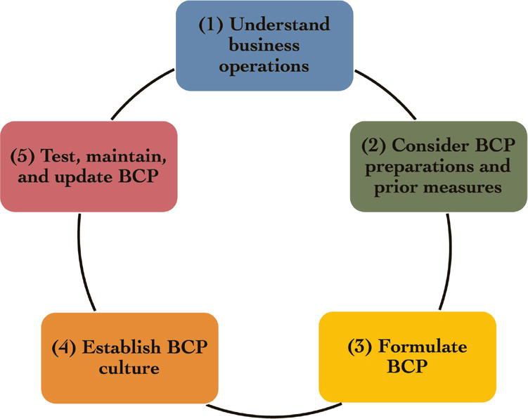
As known to all, BCP defines the activities for business continuity. It should be carried out under both normal and emergency situations to enable the business continuation or early recovery of core business operations in the event of natural disasters, major fires, terrorist attacks, or other emergency situations. With the aim of increasing the development rate of BCP in Japan, the Small and Medium Enterprise Agency has published a BCP development manual on its website, which explains how to develop a BCP for each business in detail. The process of BCP development is shown in Figure 1 [2].

Figure 1.

BCP development and operation cycle.

There are five steps for BDP development and operation, including (1) understand business operations, (2) consider BCP preparations and prior measures, (3) formulate BCP, (4) establish BCP culture, and (5) test, maintain, and update BCP. Step 2 and step 3 are considered the most important and difficult steps among all the five steps. The significance of BCP and its economic effects are mentioned to show that BCP should be a system that also could generate economic effects even in normal periods compared to conventional disaster prevention measures [3]. However, many manufacturers are stuck between step 2 and step 3. Lacking visibility of benefits under normal situations and lacking mitigation effects against losses due to supply chain disruptions are cited as the main reasons for lacking progress in BCP development.

To help manufacturers to make their decision-making on risk mitigation measures creation as well as effectiveness evaluation, research on supply chain disruption risk management (SCDRM) to deal with supply chain disruptions has been attracting much attention and the number of papers has been increasing rapidly in recent 10 years. Proposals of these papers could be broadly divided into two types which are pre-measures and post-measures. Risk assessment of supply chain structures, supplier evaluation, and procurement allocation is considered the pre-measures. On the other hand, switching to alternative components and switching procurement sources are considered the post-measures. In addition, since most of the post-measures are ineffective without any pre-measures, pre-measures can be considered as plans for post-measures.

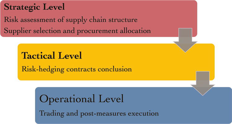
Based on the levels of decision-making, risk mitigation measures could be divided into strategic level, tactical level, and operational level. Assessing supply chain risks and determining what kind of supply chain structure should be built is considered the strategic level of decision-making. As a part of supply chain building, evaluating and selecting suppliers based on the decided supply chain structure is also considered the strategic level of decision-making. Concluding risk-hedging trading contracts, including procurement agreements, supply and penalty terms between upstream and downstream companies are considered the tactical level of decision-making. How to make post-measures more efficient is considered an operational level of decision-making. Figure 2 shows the risk mitigation measures by different decision-making levels. In this chapter, decision-making models of risk mitigation measures at the strategic level and tactical level are mainly discussed.

Figure 2.

Risk mitigation measures at different decision-making levels.

The remainder of this chapter is organized as follows. Section 2 provides an introduction to the risk assessment of supply chain structures. Section 3 provides a study on the decision-making of manufacturers on suppliers selection and procurement allocation based on the risk assessment of supply chain structures. Section 4 presents a robust and competitive contract model for manufacturers. The chapter is concluded in Section 5.

2. Risk assessment of supply chain structure

This section presents literature reviews and a previous study about risk assessment of supply chain structures [4].

The economic impact of supply chain disruptions immediately after the Great East Japan Earthquake was examined and the amount of production losses caused by the supply chain disruptions to at least 0.35% of the GDP was estimated in [5]. In ref. [6], the responses of Japanese manufacturing firms to natural disasters, such as earthquake, tsunami, and nuclear disasters, were discussed. Based on case studies, several supply-chain recovery processes after natural disasters as well as humanitarian disruptions were discussed and reflection points in terms of disaster planning, and recovery responses were summarized. In ref. [7], several supply-chain structural models were built and the tradeoff relation between supply-chain efficiency and robustness under supply-chain disruption risks was discussed. Countermeasures for mitigating supply-chain disruption risks in terms of redundancy, robustness, and flexibility were discussed after the research work on supply-chain visualization in ref. [8].

As typical natural disasters, earthquakes cause significant damage to supply chains. Since earthquakes occur frequently in Japan, procurement disruptions due to earthquakes also occur frequently. Occurrence probability, as well as impact, are two main evaluation indicators of earthquakes. In this study, the recovery period of the supply chain from the earthquake is considered as the earthquake impact. A model of procurement disruptions due to earthquakes is developed to clarify the loss difference among different supply-chain structures in Japan.

2.1 Model of procurement disruptions due to natural disasters

Although the probability of an earthquake cannot be expressed accurately, as a general thought, occurrence probability could be estimated based on historical data on earthquakes. Since earthquakes less than seismic intensity 7 only have little impact on production and procurement activities, only earthquakes with a seismic intensity of 7 or over are considered in this study.

Table 1 shows the data about earthquakes over seismic intensity 7 in the last 10 years (2011–2021) which was collected from the website of the Japan Weather Association [9]. With the data in Table 1, the average annual probability of an earthquake which seismic intensity is 7 could be estimated. Since seismic intensity 7 earthquakes occurred 4 times in 11 years including 2021, the average annual occurrence probability is 0.36 and the average monthly occurrence probability should be 0.03.

Date and time	Epicenter	Magnitude	Max seismic intensity
2018/9/6 3:08	Eastern Iburi of Hokkaido	M6.7	7
2016/4/16 1:25	Kumamoto region of Kumamoto	M7.3	7
2016/4/14 21:26	Kumamoto region of Kumamoto	M6.5	7
2011/3/11 14:46	Sanriku offshore	M7.9	7

Table 1.

Earthquakes over seismic intensity 7 in the last 10 years (2011–2021) in Japan.

In addition, the number of related areas is an important attribute of the supply chain when discussing the probability of supply-chain disruptions. In general, the larger the number of related areas of a supply chain, the higher the probability of disruption will be. Japan is divided into seven regions which are used for statistical by government officials. They are Hokkaido, Tohoku, Kanto, Chubu, Kinki, Chugoku-Shikoku, and Kyushu-Okinawa. In this study, the relation between a number of related areas of component procurement activities and the probability of disruptions is focused to verify the disruption impact. Table 2 shows the disruption probability according to the number of related areas of a supply chain. It is calculated with a number of regions and the average monthly occurrence probability of earthquakes over seismic intensity 7.

Related areas	1	2	3	4	5	6	7
Disruption probability	0.004	0.009	0.013	0.017	0.022	0.026	0.030

Table 2.

Disruption probability by related areas of supply chain.

The recovery period of the supply chain from the earthquake could also be estimated based on past earthquake occurrences. Generally, the recovery period from earthquakes depends on industry types; it is necessary to estimate the recovery period with the data which should be collected from the manufacturing industry. Table 3 shows the recovery periods of several electronic device manufacturers after the Kumamoto earthquake on April 16, 2016 [10].

Business office	Location	Date of partial recovery	Date of full recovery
Renesas Semicond. Manuf. Co., Ltd., Kawashiri factory	Kumamoto-shi	Apr. 22	May 22
FUJIFILM Kyusyu Co.,Ltd.	Kikuyomachi	Apr. 23	May 23
Mitsubishi Electric Corp. Power Device Works Kumamoto	Koushi-shi	May 9	May 31
Tokyo Electron Kyushu Ltd.	Koushi-shi	Apr. 25	End of June
Sony Semicond. Manuf. Co., Ltd., Kumamoto Tech. Ctr.	Kikuyomachi	May 9	End of July

Table 3.

Recovery dates of electronic device manufacturers after Kumamoto earthquake 2016.

The date of partial recovery in the table is the date when production activities are restarted partially. The date of full recovery in the table is the date when production activities recovered as the same as the production capacity planned beforehand. It is difficult to show the recovery of production capacity over time without the information on the recovery speed. Furthermore, it is also difficult to collect information on the recovery speed of production capacity since it is considered confidential information to manufacturers. To simplify this problem, in this study, only two conditions which are “recovered” and “not recovered” are taken into consideration, and then the average period of partial and full recovery of all manufacturers according to Table 3 is set as the estimated recovery period. With the results of the calculation, the estimated recovery period should be 36.6 days, nearly 1 month after the earthquake.

2.2 Supply chain structure models

How to build and maintain competitive supply chains is the most important task for manufacturers. In particular, manufacturers whose products are in the competition period, such as smartphones in Japan market in the 2010s, LCD TV and PC in Japan market in 2000s.

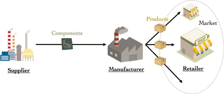
In general, manufacturers adjust their suppliers and procurement terms for the next year annually based on their strategies and evaluation results of performances in the last year. In the past, procurement plans were decided by manufacturers based on an overall evaluation of procurement cost, quality of the component, and delivery time. In most cases, the minimum number of suppliers at the lowest procurement costs was decided as the procurement plan for next year. Figure 3 shows a basic supply chain structure which is a one-supplier-one-manufacturer structure. It is considered an extreme model of a few sources supply chain. In an electronic products supply chain, such as LCD TV and smartphone, comparing with the order receiving cycle of finished products, the procurement lead time of electronic components such as LCD panel is much longer. With reference to many LCD TV and smartphone assembly manufacturers, in this supply-chain model, the order receiving cycle of products from retailers is set to 1 month, lead time of component procurement from the supplier is set to 3 months.

Figure 3.

A simple centralized procurement structure.

To analyze the impact of components procurement disruptions on the supply-chain structure, profit of the manufacturer should be the most important indicator. Eq. (1) shows the profit function of manufacturer. It is the difference between sales amount and costs including component procurement cost, inventory cost, and production cost.

$${\pi }_m=\begin{array}{l}\sum _{n=1}^N\{p_p·min\left(q_{p.n},I_{n-1}\right)-{\beta }_n{c}_{\mathit{\text{proc.}}}{q}_{c.n}-c_{\mathit{inv}.}\left(I_{n-1}+{\beta }_n{q}_{c.n}-q_{p.n}\right)\end{array}$$E1

$$-\left[c_f+c_v·min\left(q_{p.n},I_{n-1}\right)\right]\}$$

$p_p:$ Product price.

$q_{p.n}:$ Volume of product orders from the retailer.

$I_n:$ Inventory level of components.

$c_{\mathit{\text{proc}}.}:$ Component procurement cost/per unit.

$q_{c.n}:$ Volume of component procurement.

$c_{\mathit{inv}.}:$ Inventory cost/per unit.

$c_f:$ Fixed cost of production.

$c_v:$ Variable cost of production.

$N$: Period (Month).

${\beta }_n$: If there is no procurement disruption, ${\beta }_n=1$. Otherwise ${\beta }_n=0.$

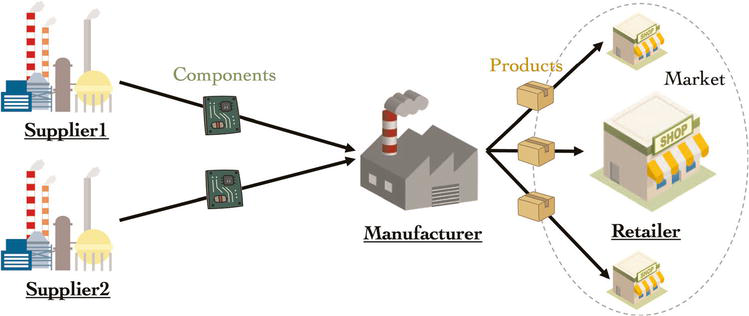
Such centralized procurement structures can help manufacturers to reduce procurement costs in normal periods. However, manufacturers are not able to achieve components in the recovery periods when a supply chain disruption occurs. It makes manufacturers a huge opportunity loss due to production stoppages. As a general robust countermeasure for hedging disruption risks, multiple sourcing has been used widely. Figure 4 shows a simplified robust procurement structure with one more supplier adding to Figure 3. If one of the procurement channels gets disrupted, the manufacturer can receive part of the total components from another supplier at least. The with this procurement structure. The manufacturer is able to keep its production facility utilization to a certain degree and avoid some opportunity losses. The profit of the manufacturer in this structure is shown in Eq. (2).

Figure 4.

A simple decentralized procurement structure.

$$\begin{array}{ll}{\pi }_m=& \sum _{n=1}^N\left\{p_p·min\left(q_{p.n},I_{n-1}\right)-{\gamma }_n{c}_{\mathit{\text{proc}}.}\left(q_{c1.n}+q_{c2.n}\right)\right.\\ & \left.-c_{\mathit{inv}.}\left[I_{n-1}-q_{p.n}+{\gamma }_n\left(q_{c1.n}+q_{c2.n}\right)\right]-\left[c_f+c_v·min\left(q_{p.n},I_{n-1}\right)\right]\right\}\end{array}$$E2

$q_{p.n}:$ Volume of product orders from the retailer

$q_{c1.n}$: Volume of component procurement from supplier 1

$q_{c2.n}$: Volume of component procurement from supplier 2

${\gamma }_n$: If there is no procurement disruption, ${\gamma }_n=1$. Otherwise ${\gamma }_n=k$

$k$: If component procurement from supplier 2 is disrupted $k=q_{c1.n}/q_{p.n}$, If component procurement from supplier 1 is disrupted $k=q_{c2.n}/q_{p.n}$. If component procurement from both suppliers is disrupted $k=0$, since the probability of such a case is extremely low, it is not considered in the experiment of this study.

In general, costs such as supplier management fees, contract fees, and ordering costs increase with the number of suppliers increasing. Although this decentralized procurement structure can be expected to reduce opportunity losses in the event of supply chain disruptions, the cost competitiveness of the supply chain is also decreased due to higher operating costs during normal periods.

2.3 Numerical experiment and results

Attributes of the supply chain, including related areas of procurement, are discussed to analyze the profit of manufacturer to clarify the difference between centralized procurement structure and decentralized procurement structure. The period of experiments is set to 3 years, and data for experiments is shown below.

Estimated product demand/month: 1000

Component procurement cost: 10,000

Component order lot size: 3000

Production cost (fixed): 10,000,000

Production cost (variable): 1000

Component procurement lead time: 3 months

Actual product demand/month: $N\left(1000,{200}^2\right)$

Product price: 35,000

Inventory cost/month: 200

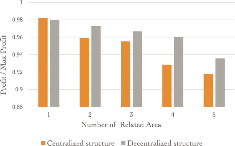
Figure 5 shows the total profit of the manufacturer which is the average value of 50 simulation runs with the number of related areas from 1 to 5. The vertical axis of the graph is the ratio of profit to maximum profit which could be achieved in a centralized procurement structure without any procurement disruptions in 3 years. From Figure 5, we can find that in more related areas of component procurement, lower profits for manufacturers in both centralized and decentralized procurement structures would be. However, comparing with a centralized structure, no significant profit reduction with increasing in related areas with a decentralized procurement structure. The effect of opportunity loss avoidance of a decentralized procurement structure is confirmed. The peak profit difference between the two structures could be confirmed in Figure 5 with the trend of increase and decrease.

Figure 5.

Total profit of manufacturer by different related areas.

3. Supplier selection and procurement allocation

Supplier selection and procurement allocation are considered one of the most important strategy level decisions to manufacturers in planning component procurement. Generally, the decision-making of supplier evaluation and selection is based on the determined supply-chain structure. This section presents literature reviews and previous work on supplier selection and procurement allocation [11].

The procurement evaluation problem which was dealt with as a multi-objective function optimization problem with randomly varying weights of cost, quality, delivery, as well as economic risks was discussed in ref. [12]. Supplier selection from all candidate suppliers by comprehensive scale assessment, including procurement risks and costs is shown in ref. [13]. In ref. [14], the problem of an optimal number of suppliers selection by considering the component inventory level under procurement lead-time uncertainty is discussed. In [15], a supplier selection method for the purpose of minimizing both procurement costs and opportunity losses was proposed. The method is based on the assumption that the component procurement price of each supplier is the same, and the order volume from each supplier is also the same. Reference [16] focused on the decoupling of recurrent supply risks and disruption risks during sourcing decisions and procurement allocation.

As decision-making of supplier selection and procurement allocation based on the decentralized procurement structure, minimum total procurement costs, including management cost, purchasing cost, transportation cost, and the opportunity cost with considering procurement disruption should be set as the objective function.

3.1 Objective functions and constraints

An optimization method for supplier selection and procurement allocation based on a one-manufacturer-multiple-suppliers supply-chain structure is proposed in this study. It is the decision-making of the manufacturer on where and how many components to procure from candidate component suppliers whose basic attributes, such as quality and delivery could meet the requirements of the manufacturer for the next period. Therefore, decision variables are set as below.

$n:$ Number of suppliers

${\mathit{ZX}}_s$: If components are sourced from the supplier $s$,${\mathit{ZX}}_s=1$. Otherwise ${\mathit{ZX}}_s=0$.

$Q_{\mathit{\text{is}}}:$ Procurement volumes of components $i$ from supplier $s$

Objective function

$${\mathit{PC}}_{\mathit{min}}=\mathit{\text{Mgmt}}.\mathit{\text{Cost}}+\mathit{Pur}.\mathit{\text{Cost}}+\mathit{\text{Trans}}.\mathit{\text{Cost}}+\mathit{\text{Oppty}}.\mathit{\text{Loss}}$$E3

As discussed before, minimum total procurement costs, including management cost, purchasing cost, transportation cost, and the opportunity cost with considering procurement disruption, are considered as the objective function. Management cost is the cost involved in managing supplier activities and contracts. It increases or decreases depending on the number of suppliers. The purchasing cost is the total cost of purchasing components from all suppliers. Transportation costs can be calculated by multiplying the unit transportation cost of each component from one supplier to the manufacturer by transportation quantity which is the same as purchasing quantity.

$$\mathit{\text{Fixed Management Cost}}=\sum _{s=1}^S\sum _{i=1}^I{\mathit{ZX}}_s\times M_s$$E4

$$\mathit{\text{Purchasing Cost}}=\sum _{s=1}^S\sum _{i=1}^I{P}_{\mathit{\text{is}}}\times Q_{\mathit{\text{is}}}$$E5

$$\mathit{\text{Transportation Cost}}=\sum _{s=1}^S\sum _{i=1}^I{\mathit{\text{Trans}}}_{\mathit{\text{is}}}\times Q_{\mathit{\text{is}}}$$E6

Eq. (7) shows the amount of opportunity loss due to any $n$ procurement channels getting disrupted. Eq. (8) shows the expected total opportunity cost which is the sum of Eq. (7)

$$C_n=\sum _{i=1}^I{L}_i\times \sum \left\{\left[D_i-min\left(D_i,\sum _{b=1}^B{Q}_{\mathit{ib}}^{\mathit{max}}\right)\right]\times \left[\prod _{a\in A_{\mathrm{n}}}{\theta }_a\times \prod _{b\in B_{\mathrm{n}}}\left(1-{\theta }_b\right)\right]\right\}$$E7

$$\text{Oppotunity Loss}=\sum _{\mathrm{n}=1}^{\mathrm{S}}{\mathrm{C}}_{\mathrm{n}}$$E8

Constraints

Equations from Eq. (9) to Eq. (11) are considered as the constraints for decision-making, including total demand for components, procurement volume from each supplier, and the number of suppliers. Eq. (9) shows the constraint of component demand. The total volume of component $i$ that could be procured from all selected suppliers should be the same as the demand for component $i$. Eq. (10) shows the constraint of component volume. The volume of component $i$ that could be procured from supplier $s$ should not be less than the minimum volume and not more than the maximum volume which is decided by supplier $s$. Eq. (11) shows the constraint of the number of suppliers available for selection. It should not exceed the number of all candidate suppliers.

$$\sum _{s=1}^S{Q}_{\mathit{\text{is}}}=D_i\forall i$$E9

$$Q_{\mathit{\text{is}}}^{\mathit{min}}\le Q_{\mathit{\text{is}}}\le Q_{\mathit{\text{is}}}^{\mathit{max}}\forall i,s$$E10

$$n\le S$$E11

$s:$ Supplier ID ($s=1,2,3,\dots ,S$)

$i:$ ID of component types ($i=1,2,3,\dots ,I$)

$D_i:$ Demand for component $i$

$M_s:$ Management cost of supplier $s$

$P_{\mathit{\text{is}}}:$ Price of component $i$ from supplier $s$ (per unit)

$Q_{\mathit{\text{is}}}^{\mathit{min}}:$ Minimum procurement volume of components $i$ from supplier $s$

$Q_{\mathit{\text{is}}}^{\mathit{max}}:$ Maximum procurement volume of components $i$ from supplier $s$

$L_i:$ Opportunity loss of components $i$ (per unit)

${\mathit{\text{Trans}}}_{\mathit{\text{is}}}:$ Transportation cost of components $i$ from supplier $s$ (per unit)

${\theta }_s:$ Disruption probability of supplier $s$ (%)

$a:$ ID of interrupted suppliers among selected suppliers ($a=1,2,3,\dots ,A$)

$b:$ ID of among selected suppliers ($b=1,2,3,\dots ,B$)

$A_n:$ The interrupted supplier group (Ex. $A_1$ indicates the group of anyone interrupted supplier)

$B_n:$ The uninterrupted supplier group (Ex. $B_1$ indicates the group of uninterrupted suppliers when any supplier is interrupted)

$Q_{\mathit{ib}}^{\mathit{max}}:$ Maximum procurement volume of components $i$ from uninterrupted suppliers

3.2 Tabu-search based decision-making

In many cases, procurement plans are decided based on the discussion in a procurement strategy meeting. As a support tool for management decisions, create and re-create supplier selection and procurement allocation plans in a short time are important. The effectiveness of Tabu-Search (TS) has been confirmed by numerous previous studies on a lot of classical optimization problems as well as practical problems. Comparing with other meta-heuristics, it is expected to search more neighborhood solutions with fewer search times. Since prohibitions are introduced to discourage search from coming back to previous-visited solutions. With considering of the applicability, a TS-based decision-making is proposed. There are five steps to decide the optimal supplier combination and procurement volume from each supplier. In this study, the average procurement cost of the supplier combination is considered as the evaluation index.

Step 1: Generate and check the initial supplier combination

Initial supplier combination according to the tentatively determined numbers of suppliers is generated randomly. The procurement amount of each component from each supplier in the initial supplier combination is set randomly based on the constraint Eq. (10).

Step 2: Check and generate neighbor solutions

Check whether or not the solution could be improved according to the evaluation index. If it could be improved, create new supplier combinations by selecting the unselected suppliers in all candidate suppliers to replace the supplier with the highest procurement cost in the supplier combination after checking the constraints as well as the Tabu list. Otherwise, proceed to Step 4.

Step 3: Update the Tabu list

Update the Tabu list by adding the supplier combination with the lowest unit cost from supplier combinations generated by Step 2.

Step 4: Adjust procurement allocation

Adjust the component volume from the supplier with the highest procurement cost to the supplier with the lowest component procurement cost by minimum adjustment unit.

Step 5: Update execution times

If the execution time $n$ is less than the total search time $N$, proceed to Step 2. Otherwise, end the execution.

3.3 Numerical experiment and results

The effectiveness of the proposed TS-based decision-making is discussed in this subsection. The data for the numerical experiment is shown below.

Number of candidate suppliers: 8

Type of components: 3

Demand for each component type: 400, 300, 200

Range of management cost: 1500–2500

Minimum procurement volume range of each component type: 60–100, 45–75, 30–50

Maximum procurement volume range of each component type: 100–180, 80–150, 60–100

Component price range of each component type/per unit: 35–52, 40–62, 49–72

Transportation cost range of each component type/per unit: 3–7, 3–7, 3–7

Disruption probability of candidate suppliers: 18–27%

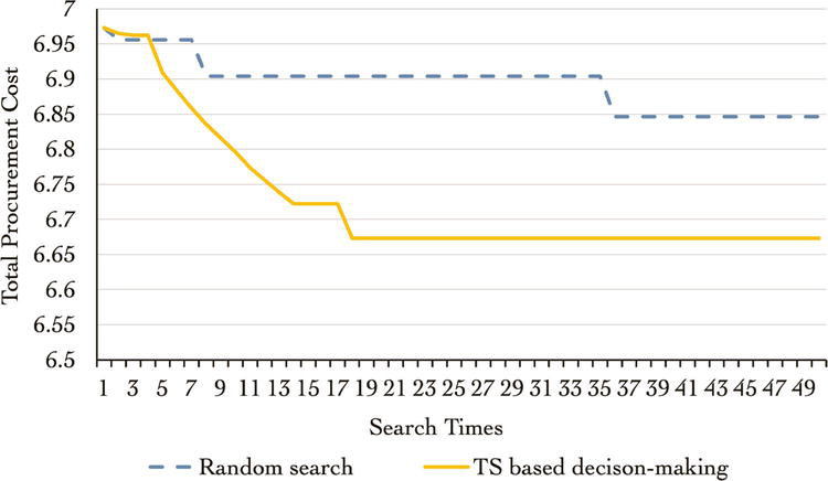
Figure 6 shows an example of the performance of TS-based decision-making against a random search in the terms of three suppliers. Comparing with random search, TS-based decision-making could reach a more accurate solution with much less search times. It could support managers to discuss and make a procurement plan efficiently in a management strategy meeting.

Figure 6.

Total procurement cost search with random search and TS-based decision-making based on three suppliers.

4. Design robust and competitive contract under disruption risks

With the results of risk assessment of supply-chain structures, as well as the results of supplier selection and procurement allocation, a trading contract between manufacturer and suppliers in which component procurement details are determined, should be discussed. In general, the procurement allocation determines the reference procurement volume of each component from each supplier. A trading contract that is concluded between manufacturer and supplier determines the terms of component trading. The manufacturer procures components from the supplier based on the estimated demand for a decided period. According to the example of LCD TV and smartphone assembly industry mentioned in Section 2, if the order-receiving cycle of products from retailers is 1 month and the lead time of component procurement from the supplier is 3 months, the manufacturer should place an order to the supplier with considering of the estimated demand for one month after the next 3 months and its component inventory.

Risk assessment of supply-chain structures and supplier selection and procurement allocation with risk evaluation can help manufacturers to reduce their procurement risks, but they could not help manufacturers to alleviate their losses in the event of a supply disruption. A robust and competitive procurement contract with post-measures execution consideration is also necessary for manufacturers. Many previous studies discussed the effectiveness of options contracts in managing supply-chain disruption risks. In ref. [17], a model for a three-echelon supply chain including two different manufacturers, one distributer and one retailer, to analyze the effect of the combination of option and buyback contracts under supply-disruption risk was created. In ref. [18], a supply-chain problem where a buyer receives a product from a cheap but unreliable main supplier and signs an option contract with a perfectly reliable backup supplier to share supply and demand uncertainty was discussed. A mechanism was developed to maximize system efficiency and a win–win relationship between supplier and buyer based on an optimization problem with option contracts. Reference [19] focused on a supply chain including a manufacturer who faces stochastic demand, an overseas module supplier, and two local module suppliers. The overseas supplier offers high-quality products while being susceptible to disruption risks. Though local suppliers have high reliability, it may decrease sharply if they offer products of lower quality. Optimal order volume and reservation volume of the manufacturer based on capacity reservation contract were derived.

The purpose of the contracts discussed above is to give procurement volume an adjustable range to avoid loss caused by uncertainties including supply disruptions. If this adjustable range is large enough, manufacturers can procure the necessary quantity of parts based on fluctuations in demand, and part of the loss caused by disruption can be covered by procuring the maximum level of the adjustable range from other suppliers.

4.1 Robust and competitive contract model

To realize such an adjustable range for procurement, it is necessary for manufacturers to make a lump-sum payment to suppliers to determine the upper limit of procurement volume in advance. On the other hand, the higher the upper limit of the procurement volume range is, the supplier has to bear more inventory risk. Generally, the lump-sum amount is decided by the supplier with considering the inventory risk based on the upper limit of procurement volume.

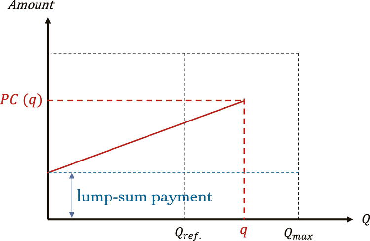
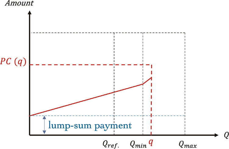
Figure 7 shows the structure of trading volume and price with the upper limit of procurement volume that is dependent on the amount of lump-sum payment. $Q_{\mathit{ref}.}$ is the reference volume decided by the manufacturer due to the decision on procurement allocation. $Q_{\mathit{max}}$ is an upper limit of procurement volume. $\mathit{PC}\left(q\right)$ is the total value of the lump-sum payment amount and $c_{\mathit{\text{proc}}.}$ which is the procurement amount with procurement volume $q$.

Figure 7.

Structure of trading volume and price with the lump-sum payment.

Eq. (12) shows the profit of the manufacturer with this contract structure based on the simple decentralized procurement structure, as shown in Figure 4. It is similar to Eq. (2). With the lump-sum payment ${\mathit{ls}}_1$ and ${\mathit{ls}}_2$ to supplier 1 and supplier 2, the manufacturer can make the decision on procurement volume with a wider adjustable range each time.

$$\begin{array}{ll}{\pi }_m=& \sum _{n=1}^N\left\{p_p·min\left(q_{p.n},I_{n-1}\right)-\left({\mathit{ls}}_1+{\mathit{ls}}_2\right)-{\gamma }_n{c}_{\mathit{\text{proc}}.}\left(q_{c1.n}+q_{c2.n}\right)\right.\\ & \left.-c_{\mathit{inv}.}\left[I_{n-1}-q_{p.n}+{\gamma }_n\left(q_{c1.n}+q_{c2.n}\right)\right]-\left[c_f+c_v·min\left(q_{p.n},I_{n-1}\right)\right]\right\}\end{array}$$E12

${\mathit{ls}}_1:$ Lump-sum payment to supplier 1.

${\mathit{ls}}_2:$ Lump-sum payment to supplier 2.

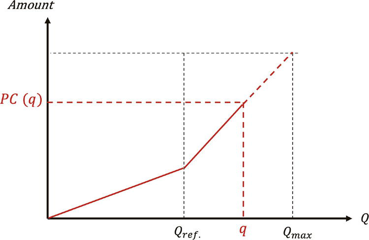
The contract structure shown in Figure 7 with an adjustable range for procurement could be considered a robust method, however, the lump-sum payment makes the manufacturer cost extra expenses when the required volume of components is less than the reference volume or no procurement disruptions occur. The determination of procurement volume by lump-sum payments makes the price competitiveness of the manufacturer lower. To improve the problem, a structure of 2-stage procurement cost without lump-sum payments is proposed in this study. Figure 8 shows the concept of the contract structure.

Figure 8.

Structure of 2-stage procurement cost.

Instead of lump-sum payments, the manufacturer should procure components at a higher unit price than the normal procurement price when the procurement volume is more than the reference procurement volume according to the result of procurement allocation. $\mathit{PC}\left(q\right)$ is the total value of $Q_{\mathit{ref}.}$with normal procurement price and procurement price to the additional volume of $\left(q-Q_{\mathit{ref}.}\right)$. Moreover, the upper limit of procurement volume is determined by the supplier considering the unit price of the additional procurement volume. The higher the price of the additional procurement volume is the incentive of the supplier for setting a higher upper limit would be higher.

Eq. (13) shows the profit of the manufacturer with this contract structure while $q_{c.n}\le Q_{\mathit{ref}.}$. Eq. (14) shows the profit of the manufacturer with this contract structure while $Q_{\mathit{ref}.}<q_{c.n}\le Q_{\mathit{max}}$.

$$\begin{array}{l}{\pi }_m=\sum _{n=1}^N\{p_p·min\left(q_{p.n},I_{n-1}\right)-{\gamma }_n{c}_{\mathit{\text{proc.}}}\left(q_{c1.n}+q_{c2.n}\right)\\ -c_{\mathit{inv}.}\left[I_{n-1}-q_{p.n}+{\gamma }_n\left(q_{c1.n}+q_{c2.n}\right)\right]-\left[c_f+c_v·min\left(q_{p.n},I_{n-1}\right)\right]\}\end{array}$$E13

$$\begin{array}{l}{\pi }_m=\sum _{n=1}^N\{p_p·min\left(q_{p.n},I_{n-1}\right)-{\gamma }_n{c}_{\mathit{\text{proc.}}}\left(Q_{\mathit{ref}.1}+Q_{\mathit{ref}.2}\right)\end{array}$$E14

$$\begin{array}{c}-{\gamma }_n{c}_{\mathit{\text{proc.}}}^{\prime }\left(q_{c1.n}+q_{c2.n}-Q_{\mathit{ref}.1}-Q_{\mathit{ref}.2}\right)-c_{\mathit{inv}.}\left[I_{n-1}-q_{p.n}+{\gamma }_n\left(q_{c1.n}+q_{c2.n}\right)\right]\\ -\left[c_f+c_v·min\left(q_{p.n},I_{n-1}\right)\right]\}\end{array}$$

$Q_{\mathit{ref}.1}$: Reference procurement volume of supplier 1.

$Q_{\mathit{ref}.2}$: Reference procurement volume of supplier 2.

$c_{\mathit{\text{proc}}.}:$ Normal component procurement unit cost.

$c_{\mathit{\text{proc}}.}^{\prime }$: Component procurement unit cost for additional volume

It is considered that the competitiveness of the contract structure which is shown in Figure 7 should be higher than the contract structure which is shown in Figure 8 when product demand is in an expanding trend with high fluctuation. On the other hand, when product demand is in a stable trend with low fluctuation, it is considered that the competitiveness of the contract structure which is shown in Figure 8 should be higher than the contract structure which is shown in Figure 7.

As shown in Figure 9, it is a combination structure of lump-sum payments and 2-stage procurement cost. The amount of lump-sum payments and procurement price to the additional volume are adjusted by the manufacturer with considering the features of product demand. The supplier should guarantee its supply volume by or over $Q_{\mathit{min}}$ according to the amounts of lump-sum payments. It helps manufacturers to expand the range of procurement volume that can be procured reliably. Moreover, the 2-stage procurement cost gives the supplier the incentive to set its maximum component supply volume.

Figure 9.

Structure of lump-sum payment and 2-stage procurement cost.

Profit of manufacturer with this contract structure could be expressed by Eq. (12) while $q_{c.n}\le Q_{\mathit{min}.}$. Eq. (15) shows the profit of the manufacturer with this contract structure while $Q_{\mathit{min}}<q_{c.n}\le Q_{\mathit{max}}$.

$$\begin{array}{l}{\pi }_m=\sum _{n=1}^N\{p_p·min\left(q_{p.n},I_{n-1}\right)-\left({\mathit{ls}}_1+{\mathit{ls}}_2\right)-{\gamma }_n{c}_{\mathit{\text{proc.}}}\left(Q_{\mathit{min}.1}+Q_{\mathit{min}.2}\right)\end{array}$$E15

$$\begin{array}{c}-{\gamma }_n{c}_{\mathit{\text{proc.}}}^{\prime }\left(q_{c1.n}+q_{c2.n}-Q_{\mathit{min}.1}-Q_{\mathit{min}.2}\right)-c_{\mathit{inv}.}\left[I_{n-1}-q_{p.n}+{\gamma }_n\left(q_{c1.n}+q_{c2.n}\right)\right]\\ -\left[c_f+c_v·min\left(q_{p.n},I_{n-1}\right)\right]\}\end{array}$$

4.2 Numerical experiment and results

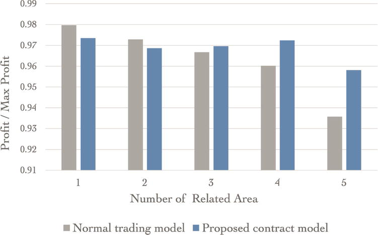
The experiment environment is set as the same as in Section 2.3. It is considered that there are no differences in lump-sum payment, procurement volume and $Q_{\mathit{min}}$ between two suppliers. Besides the experiment data in Section 2.3, $Q_{\mathit{min}}$ is set to 10% more than the component order lot size, lump-sum payment is set as the component inventory cost of the difference between $Q_{\mathit{min}}$ and order lot size. Figure 10 shows an example of a numerical experiment result.

Figure 10.

Total profit of manufacturer by different related areas with normal trading model and proposed contract model.

The vertical and horizontal axes of Figure 10 are set as the same as in Figure 5. The results in Figure 10 are also the average value of 50 simulation runs. The normal trading model is the model in which the manufacturer places an order to the supplier based on the estimated product demand, and the supplier supplies components according to the order at a pre-determined trading price. On the other hand, the proposed contract model is the contract structure of lump-sum payment and 2-stage procurement cost. From Figure 10, it could be found that with the proposed contract model, there is no significant reduction in profit with increasing in related areas.

5. Conclusions

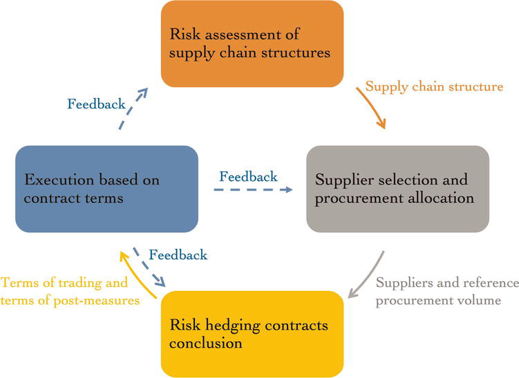
As discussed in Section 1, many manufacturers are stuck between step 2 and step 3 of the BDP development and operation cycle. Lack of visibility of benefits under normal situations as well as mitigation effects against losses due to supply chain disruptions is considered the main reasons. Figure 11 shows the detail of Figure 2 which is the summary of prior measures discussion and design. In this chapter, except for the process of execution based on contract terms, the hierarchy of prior measures and ideas on specific measures, including risk assessment of supply-chain structures, supplier selection, procurement allocation, and risk-hedging contracts conclusion, is proposed. The effectiveness of these proposed measures is confirmed by numerical experiments.

Figure 11.

Summary of prior measures discussion and design.

In Section 2, the profit of manufacturers with a centralized procurement structure model and decentralized procurement structure model is confirmed under supply-chain disruption risks due to earthquakes in Japan. The loss aversion effect of a decentralized procurement structure is confirmed quantitatively. In Section 3, a decision-making method for a decentralized procurement structure is proposed based on Tabu Search. It is confirmed that it could help decision-makers to make more accurate solutions effectively in supplier selection and procurement allocation. In Section 4, the lump-sum payment and 2-stage procurement cost structure contract model based on the selected suppliers and the results of procurement allocation is proposed. It could help manufacturers to solve the problem of securing procurement volume while falling in procurement disruptions and the problem of keeping procurement at low cost even in normal periods.

Market power and cooperation level between upstream and downstream companies are necessary to be considered in designing and planning supply chains. Furthermore, all of the analyses and proposals in this chapter are from the perspective of the manufacturer. Actually, a robust and competitive supply chain could not be built and kept without cooperation from suppliers. Therefore, analysis from the perspective of the supplier to clarify the conditions for realizing a win–win relationship is also an important task.

Nomenclature list

$p_p$

Product price

$q_{p.n}$

Volume of product orders from the retailer

$I_n$

Inventory level of components

$c_{\mathit{\text{proc}}.}$

Component procurement cost/per unit

$q_{c.n}$

Volume of component procurement

$c_{\mathit{inv}.}$

Inventory cost/per unit

$c_f$

Fixed cost of production

$c_v$

Variable cost of production

$N$

Period (Month)

$q_{p.n}$

Volume of product orders from the retailer

$q_{c1.n}$

Volume of component procurement from supplier 1

$q_{c2.n}$

Volume of component procurement from supplier 2

${\beta }_n$

If there is no procurement disruption, ${\beta }_n=1$. Otherwise ${\beta }_n=0$

${\gamma }_n$

If there is no procurement disruption, ${\gamma }_n=1$. Otherwise ${\gamma }_n=k$, If component procurement from supplier 2 is disrupted $k=q_{c1.n}/q_{p.n}$, and if component procurement from supplier 1 is disrupted $k=q_{c2.n}/q_{p.n}$. Otherwise, $k=0$ since the probability of such a case is extremely low, it is not considered in the experiment of this study.

$n$

Number of suppliers

${\mathit{ZX}}_s$

If components are sourced from the supplier $s$,${\mathit{ZX}}_s=1$. Otherwise ${\mathit{ZX}}_s=0$.

$Q_{\mathit{\text{is}}}$

Procurement volumes of components $i$ from supplier $s$

$s$

Supplier ID ($s=1,2,3,\dots ,S$)

$i$

ID of component types ($i=1,2,3,\dots ,I$)

$D_i$

Demand for component $i$

$M_s$

Management cost of supplier $s$

$P_{\mathit{\text{is}}}$

Price of component $i$ from supplier $s$ (per unit)

$Q_{\mathit{\text{is}}}^{\mathit{min}}$

Minimum procurement volume of components $i$ from supplier $s$

$Q_{\mathit{\text{is}}}^{\mathit{max}}$

Maximum procurement volume of components $i$ from supplier $s$

$L_i$

Opportunity loss of components $i$ (per unit)

${\mathit{\text{Trans}}}_{\mathit{\text{is}}}$

Transportation cost of components $i$ from supplier $s$ (per unit)

${\theta }_s$

Disruption probability of supplier $s$ (%)

$a$

ID of interrupted suppliers among selected suppliers ($a=1,2,3,\dots ,A$)

$b$

ID of among selected suppliers ($b=1,2,3,\dots ,B$)

$A_n$

The interrupted supplier group (Ex. $A_1$ indicates the group of anyone interrupted supplier)

$B_n$

The uninterrupted supplier group (Ex. $B_1$ indicates the group of uninterrupted suppliers when any supplier is interrupted)

$Q_{\mathit{ib}}^{\mathit{max}}$

Maximum procurement volume of components $i$ from uninterrupted suppliers

$C_n$

The amount of opportunity loss due to any $n$ procurement channels getting disrupted

$Q_{\mathit{max}}$

Upper limit of procurement volume determined by the supplier according to the unit price of the additional procurement volume

${\mathit{ls}}_1$

Lump-sum payment to supplier 1

${\mathit{ls}}_2$

Lump-sum payment to supplier 2

$p_p$

Product price

$q_{p.n}$

Volume of product orders from the retailer

$I_n$

Inventory level of components

$c_{\mathit{\text{proc}}.}$

Component procurement cost/per unit

$c_{\mathit{inv}.}$

Inventory cost/per unit

$c_f$

Fixed cost of production

$c_v$

Variable cost of production

$N$

Period (Month)

$Q_{\mathit{ref}.1}$

Reference procurement volume of supplier 1

$Q_{\mathit{ref}.2}$

Reference procurement volume of supplier 2

$c_{\mathit{\text{proc}}.}^{\prime }$

Component procurement unit cost for additional volume

$q_{c.n}$

Volume of component procurement

$q_{c1.n}$

Volume of component procurement from supplier 1

$q_{c2.n}$

Volume of component procurement from supplier 2

$Q_{\mathit{min}.1}$

Upper limit of procurement volume from supplier 1 according to the amounts of lump-sum payments to supplier 1

$Q_{\mathit{min}.2}$

Upper limit of procurement volume from supplier 2 according to the amounts of lump-sum payments to supplier 2

$Q_{\mathit{max}}$

Upper limit of procurement volume determined by the supplier according to the unit price of the additional procurement volume

${\gamma }_n$

If there is no procurement disruption, ${\gamma }_n=1$. Otherwise ${\gamma }_n=k$, If component procurement from supplier 2 is disrupted $k=q_{c1.n}/q_{p.n}$, and if component procurement from supplier 1 is disrupted $k=q_{c2.n}/q_{p.n}$. Otherwise, $k=0$ since the probability of such a case is extremely low, it is not considered in the experiment of this study.

References

1.Business Policy Forum. Survey Report on Improving the Effectiveness of Corporate Business Continuity in the Wake of the Great East Japan Earthquake [Internet]. 2013. Available from: https://www.bpfj.jp/report/manufacturing_h24/ [Accessed: 2022-02-25]
2.The Small and Medium Enterprise Agency. Guidebook on SME Business Continuity Planning [Internet]. 2008. Available from: https://www.chusho.meti.go.jp/keiei/antei/download/bcp_guide.pdf. [Accessed: 2022-02-25]
3.Maruya H, zigyou keizokukeikaku no igitokeizaikouka: heizyouzi ni hyoukasareru zissenmanezimenntohe (in Japanese). Tankobon. Gyosei; 2008. p. 244
4.Matsuno K, Hosokawa N, Ohno T. Business analysis of electronic device manufacturers on business continuity plans under uncertain supply chain disruption risks. In: E-Proceedings of the 26th International Conference on Production Research (26th ICPR). Taichung; 18-21 July 2021
5.Tokui J, Kawasaki K, Miyagawa T. The economic impact of supply chain disruptions from the great East-Japan earthquake. Japan and the World Economy. 2017;41:59-70. DOI: 10.1016/j.japwor.2016.12.005
6.Park Y, Hong P, Roh JJ. Supply chain lessons from the catastrophic natural disaster in Japan. Business Horizons. 2013;56:75-85. DOI: 10.1016/j.bushor.2012.09.008
7.Masuda T, Mizuno H. Study for risk management of disruption in supply chains. Proceedings of the School of Information and Telecommunication Engineering Tokai University. 2017;10(1):25-35
8.Matsukawa H, Liu T. A supply chain visualization system and its validation analysis. Journal of Japan Industrial Management Association. 2016;67(2):73-82. DOI: https://doi.org/10.11221/jima.67.73
9.Japan Weather Association: Historical Information of Earthquakes [Internet]. Available from: https://earthquake.tenki.jp/bousai/earthquake/entries/level-6-plus/. [Accessed: 2022-02-27]
10.Kashima H. The 2016 Kumamoto earthquake and manufacturing industry: Regional characteristics on the disasters and restoration processes. Annals of the Association of Economic Geographers. 2018;64(2):138-149. DOI: https://doi.org/10.20592/jaeg.64.2_138
11.Matsuno K, Weng J, Shao X. Sourcing decision with capacity reservation under supply disruption risk. Asian Journal of Management Science and Applications. 2021;6(1):49-68. DOI: 10.1504/AJMSA.2021.118403
12.Moghaddam KS. Fuzzy multi-objective model for supplier selection and order allocation in reverse logistics systems under supply and demand uncertainty. Expert Systems with Applications. 2015;42(15–16):6237-6254. DOI: 10.1016/j.eswa.2015.02.010
13.Arabsheybani A, Paydar MM, Safaei SA. An integrated fuzzy MOORA method and FMEA technique for sustainable supplier selection considering quantity discounts and supplier’s risk. Journal of Cleaner Production. 2018;190:577-591. DOI: 10.1016/j.jclepro.2018.04.167
14.Abginehchi S, Farahani Z. R: Modelling and analysis for determining optimal suppliers under stochastic lead times. Applied Mathematical Modelling. 2010;34(5):1311-1328. DOI: 10.1016/j.apm.2009.08.021
15.Meena P, Sarmah PS, Sarkar A. Sourcing decisions under risks of catastrophic event disruptions. Transportation Research Part E: Logistics and Transportation Review. 2011;47(6):1058-1074. DOI: 10.1016/j.tre.2011.03.003
16.Chopra S, Reinhardt G, Mohan U. The importance of decoupling recurrent and disruption risks in a supply chain. Naval Research Logistics. 2007;54(5):544-555. DOI: 10.1002/nav.20228
17.Shu T, Yang F, Chen S, Wang S, Lai KK, Gan L. Contract coordination in dual sourcing supply chain under supply disruption risk. Mathematical Problems in Engineering. 2015;2015(7):1-10. DOI: 10.1155/2015/473212
18.Asian S, Nie X. Coordination in supply chains with uncertain demand and disruption risks: Existence, analysis, and insights. IEEE Transactions on Systems, Man, and Cybernetics: Systems. 2014;44(9):1139-1154. DOI: 10.1109/TSMC.2014.2313121
19.Hou J, Zeng AZ, Sun L. Backup sourcing with capacity reservation under uncertain disruption risk and minimum order quantity. Computers and Industrial Engineering. 2017;103:216-226. DOI: 10.1016/j.cie.2016.11.011
Written By
Kotomichi Matsuno, Jiahua Weng, Noriyuki Hosokawa and Takahiro Ohno
Submitted: 03 April 2022Reviewed: 21 April 2022Published: 24 June 2022
Open access peer-reviewed chapter