Facility Location

Abstract

The location of the production, distribution and storage facilities of organizations, remains one of the most important strategic decision production and operations managers have to make. Minimizing total cost and distance traveled is the fundamental objective in deciding the location of facilities in order to maximize total profit. There are several quantitative methods for solving facility location problems and deciding on the most optimal decision to reach as it regards locating a facility or assigning workers to their most optimal location or tasks. The Linear Assignment model with particular emphasis on the Hungarian and Branch and Bound technique under minimization and maximization situations are deterministic approaches to solving facility location problems and have been discussed in this chapter.

1. Introduction

Facility Location is an important factor in the supply chain that significantly impacts on the efficiency and effectiveness of many supply networks and the organization at large. Location decisions are strategic in character, long-term in nature, and non-repetitive in nature. Without good and thorough site planning from the start, the new facilities may have ongoing operational issues in the future. Poor Location decision not only affects the growth of the firm but impedes on the growth and development of the nation. The location decision should be made with great care, as any error that results in a poor location can be a constant source of higher costs, higher investment, difficult marketing and transportation, dissatisfied and frustrated employees and consumers, frequent interruptions of production, abnormal wastages, delays, and substandard quality, among other things.

Facility location significantly impacts on revenue, costs, and service levels to customers. It is thus a classical optimization problem for determining the sites for factories, service outlets and warehouses. Facility location decision is made by selecting the best option among a set of possible sites depending on the nature or type of business. The choice of facility location is strategically guided by profit maximization or minimization of all costs associated with the choice of location.

2. Facility location planning

Facility location is connected with capacity decisions. Capacity expansion considerations instantly raises the twin issue of where to expand in order to tie in effectively with the distribution network of facility location. Facility location of operations is a long-term capacity decision which involves huge and long term commitment about the geographically fixed factors that affects business organizations. The selection of location is therefore a key-decision of production and operations managers as large investment is made in building plant and machinery.

Cambridge dictionary defined a facility as “a place, especially including buildings, where a particular activity happens”. Facility extends beyond a place or a building, it includes structures, equipment, or people. It also includes hospitals, food production plants, and gas stations among others. Adeleke and Olukanmi [1] suggested that facility location issues seeks to determine how to locate a number of facilities from a set of potential facilities that will serve a number of customers. Alenezy [2] added that the cost-effective site is to be chosen from the potential locations in which to place new facilities or retain existing ones.

Facility location can therefore be defined as the siting of facilities which could be structures, men, material, machines in such a manner that yields an optimum benefit to the firm and its stakeholders. There are two major location decisions or problems faced by managers, they are internal and external location problems. Internal location problems are concerned with decisions on where to locate facilities inside the plant. A good example of an internal location decision is where to place a new machine or storage room within the existing facility. Internal facility location decision deals with the assignment or location of facility whose space constraint is equal to or smaller than the available space existing within the facility. An external location decision on the other hand deals with the problem of where to site a new manufacturing plant, warehouse, building, or a new branch within an agreed geographical area [3, 4, 5, 6, 7].

The following circumstances may necessitate facility location decisions:

1. Upon the commencement of a new business or gaining entrance

2. When an established company outgrows its existing facility and expansion is no longer feasible, a new location decision is made.

3. Expansion of current firm or market size that demands the opening of new branches.

4. Insecurity issues

5. Creation/development of a new product.

6. Government policies.

7. When a lease ends without being renewed by the landlord.

8. Social or financial considerations

When expansion is inevitable three options are open to an organization

• Expand on the current location of land/facilities available

• Look for a new space and use it as an extension of the other office

• Look for a large portion of land that can accommodate both the existing business and the new line of business

3. Importance of location decision

1. Location study helps to find the optimal location of organization facility or plant that will result in the greatest advantage to the organization.

2. Location plays a huge role in attracting and retaining the best employees, that gives a competitive edge over the firm’s rival

3. A good location decision helps in avoiding waste of all the investments made in plant and machinery equipment.

4. A good location decision helps to optimize performance of the firm by minimizing its total cost of production.

5. It also ensures safety for its workforce

6. Locating a facility in the right place can give access to customers and also enable the firm enjoy incentives provided by government

4. Factors to consider when taking a location decision

There are several factors that must be critically analyzed when considering locating a facility. These factors can be grouped into two categories: controllable and uncontrollable factors.

4.1 Controllable factors

1. Availability of Inputs: This is a major decision guiding facility location problems. Manufacturing companies that use heavy, bulky or perishable products as raw materials or factor inputs have to be located near the source of these raw materials or inputs, this is to ensure regular and timely supply of raw materials as well as reduce the cost of transporting and storing them. A good example are food processing companies, the major farm product used in processing those goods need to be in close range to ensure steady supply of these products. Similarly, most wood processing companies are located close to the supply of quality timber. Generally, the cost of transportation or shipping of these raw material is to be weighed. Perishable products may be lost or damaged in transit if the distance to the plant is far, thus the closer the facility is to the source of its inputs determines its ability to cut costs.

2. Market/Customer Proximity: Goods are produces to be sold to the identified markets or customers, therefore the proximity of a facility to the market or customers is of grave importance to the organization. Proximity helps to reduce transportation costs and time of delivery.

3. Integration with Other Parts of the Organization: It is of significant benefit to keep a new plant or subsidiary plant close to the parent facility. This makes it easier for them to share resources and thus reduce total cost.

4. Availability of Labor and Skills: Education, experience and skill of available labour is an important factor that affects location decision. It is always preferable to locate the plant in an area where skilled, semi-skilled and unskilled labour are available. This reduces costs of training and hiring experts from abroad

5. Availability of Amenities: Good roads, hospitals, school’s churches, parks and residential area are necessary amenities that make living conditions for worker’s desirable.

6. Availability of Transportation Facilities: Good transportation facilities makes the plants accessible for easy movement of raw materials as well as finished products, thereby reducing costs.

7. Availability of Services: The availability of basic support services needed by the facility to make their operations smooth should be considered. This decision affects to total cost of operation, where such services are not readily available or at a high cost, the organization will have to spend more in providing such services, or attracting them at a higher cost.

8. Room for Expansion: The possibility of increasing future production capacity occasioned by increase in product demand is a critical factor in location decisions. There should be adequate space for future expansion or diversification of the facility as the need arises.

9. Safety: The safety of employees as well as the facility needs to be taken into consideration when making location decisions. If the location is not safe, it may detract employees and even potential customers from patronizing the facility. Also, the probability of loss of property, or damage of the machines increases when safety of the environment or location is poor.

4.2 Uncontrollable factors

1. Community and labour attitude: Communities that are interested in attracting new plants may offer reduced prices or no cost sites to companies as a way of growing their communities. The cost of land and attitude of labour to work is a major factor to consider when making location decisions.

2. Suitability of Land and Climate: Due consideration should be given to the suitability of the land and climate for the nature of the products and the type of machines used in production. If the climate in a given geographical location does not support the product type it may lead to wastage in the long run, hence due consideration should be given to this factor.

3. Regional Regulations: The regulations in certain regions do not support the production of certain types of products or services, organizations should investigate the regulations of the desired region before going ahead to site their plants or facility.

4. Political, Cultural and Economic Situation: The political, cultural and economic situation of the location should be well considered. Areas notable for political unrest, may not favor the facility as protests and other activities may lead to the damage of the facility. Also, some cultures are noted for certain behaviors that may not be compatible with the activities of the plant. Lastly, economic situation in a given location may stall the growth of the organization in the short and long run.

5. Power supply: Cost and quality of power supply is a high importance in the location of a plant. Cost of power supply is usually cheaper at rural locations than the urban areas. Some companies generate their own power. The overall cost of power supply should be taken into consideration when making facility location decisions.

6. Regional Taxes, Special Grants and Import/Export Barrier: The kind and amount of taxes levied by a state should be considered in locating a plant/facility. Investigation should be made on the type of taxes and the biases for which they are fixed. Some places have special grants given to attract investors to such area. Similarly, import/export barriers should be duly considered as this affects the total cost of doing business.

7. Government Policies: The policies of the state governments and local bodies concerning labor laws, building codes, safety, etc., are the factors that demand attention. In order to have a balanced regional growth of industries, both central and state governments in our country offer the package of incentives to entrepreneurs in particular locations. The incentive package may be in the form of exemption from a sales tax and excise duties for a specific period, soft loan from financial institutions, subsidy in electricity charges and investment subsidy. Some of these incentives may tempt to locate the plant to avail these facilities offered.

5. Solution methods for location problem

There are various approaches for solving location problems such as:

1. The Dimensional Analysis approach

2. The Simple ranking of alternative site approach

3. The Linear Assignment model

4. The Linear Transportation model

5. The Quadratic Assignment model

6. The Heuristic solution procedure

The solution method we shall focus on is the Linear Assignment model.

6. Linear assignment model

Linear assignment model (LAM) is a deterministic mathematical model applied when the management decides to make an optimum use of its capacity. It is referred to as being linear because there is always a straight line relationship between the variable involved. There are two major objectives which linear assignment model can seek to achieve;

1. Maximization of profit

2. Minimization of cost

There are two major methods for solving linear assignment model

1. Hungarian method

2. Branch and Bound technique

6.1 Hungarian method

The Hungarian method is one of the many algorithms that have been devised to solve linear assignment problem.

To solve identified problem, the number of assignment must be equal to the number of people or machines to do the job. However, if there is a shortfall in either in the available job or persons/machines to do the job. A dummy row or column is created before carrying out the various iterations to solve the problem.

6.1.1 Procedures for solving minimization problems

When dealing with minimization objective under the Hungarian method, it is critical to ensure that the scenario in the case is a minimization situation. If the question focusses on cost, risk, distance covered etcetera then it is a minimization question and the following ten simple steps can be applied.

Step 1: Write out the initial matrix and check whether the number of row is equal to the number of columns. Create a dummy row or column where necessary.

Step 2: Perform row reduction by identifying the smallest element in each row and deduct the identified element from the other element in the row. Do same for all the rows.

Step 3: Perform a column reduction by identifying the smallest element in each column and deducting it from all other element. Apply to all columns. Please note this is to be done on the most recent matrix after the row reduction and not on the initial matrix.

Step 4: identify the number of unique zero’s in each selected row and column.

Step 5: Apply the minimum number of possible lines on the unique zero’s starting with either the row or column with the highest number of unique zero’s. Where there are ties, they are broken arbitrarily. Note: do not cover any unique zero twice.

Step 6: Count the number of minimum possible lines and compare with the number of assignment to be performed i.e. M = N = Minimum number of lines ruled (//).

Where M = Persons or machines to be assigned the task.

N = Assigned task.

Step 7: If M = N= // (optimality had been attained). Jobs can then be assigned to workstations or locations but if M ≠ N ≠//or if M = N ≠// (optimality is not attained). The iteration process should be continued.

Step 8: If optimality is not attained then identify the smallest uncovered element in the matrix and deduct same from other uncovered elements in the matrix, but add the identified smallest uncovered element to the elements at the point of intersection of the straight lines.

Step 9: Repeat steps 4, 5, 6 above until optimality is attained (i.e M = N= //).

Step 10: Assign jobs starting with the row with a single unique zero and pick the corresponding value in the initial matrix.

Example 1

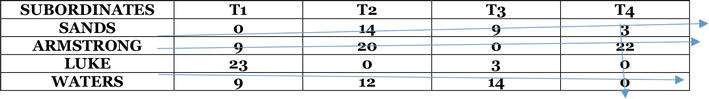
A Plant manager has four subordinates and four tasks to be performed. The subordinates differ in efficiency and the tasks differ in their intrinsic difficulty. The estimate of the time each man would take to perform each task is given in the effectiveness matrix below. The objective is to assign men to jobs in such a way that the total time taken to complete an assignment is minimized (see Table 1).

Subordinates	T1	T2	T3	T4
Sands	8	26	17	11
Armstrong	13	28	4	26
Luke	38	19	18	15
Waters	19	26	24	10

Table 1.

Cost matrix.

Solution:

(see Tables 2–5).

Subordinates	T1	T2	T3	T4	Smallest element in a row
Sands	8	26	17	11	8
Armstrong	13	28	4	26	4
Luke	38	19	18	15	15
Waters	19	26	24	10	10

Table 2.

Initial tableau.

Subordinates	T1	T2	T3	T4
Sands	0	18	9	3
Armstrong	9	24	0	22
Luke	23	4	3	0
Waters	9	16	14	0
Smallest element in a column	0	4	0	0

Table 3.

Row reduction matrix.

Subordinates	T1	T2	T3	T4
Sands	0	14	9	3
Armstrong	9	20	0	22
Luke	23	0	3	0
Waters	9	12	14	0

Table 4.

Column reduction matrix.

Table 5.

Straight line tableau.

Test for optimality

M = N = No of lines

4 = 4 = 4

From the table above, all the zeros in the rows and columns have been covered by four straight lines. Hence, the optimal solution has been reached and we can now make an optimal assignment following the pattern of unique zeros (see Table 6).

Subordinates	Possible tasks	Assigned tasks	Time
Sands	T1	T1	8
Armstrong	T3	T3	4
Luke	T2; T4	T2	19
Waters	T4	T4	10
			41 HOURS; (OPTIMAL)

Table 6.

Assignment table.

The assignment should begin with the subordinate with only one possible task based on the number of unique zeros on each row. From the straight line table we can see that Sands, Armstrong and Waters have one unique zero on their respective rows, hence we assign Sands to Task 1, Armstrong to T3 and Waters to T4. Luke has two unique zeros on the row indicating two possible assignments (T2 and T4) since T4 has already been assigned to Waters (being the only possible assignment to Waters) we can no longer assign it to another subordinate, we then assign T2 to Luke. The summary of our assignment is shown above.

Example 2

The management of Cadbury Plc is interested in assigning her newly employed operations managers to her newly established branches in four different locations in Africa (Nigeria, Ghana, South Africa and Kenya). The cost implication and profit are of interest to the firm. However, the management desires to focus on cost (see Table 7).

Managers/Location	Nigeria	Ghana	SA	Kenya
Mike	950	610	980	360
Sultan	960	760	890	1040
Emmanuel	600	940	670	850
Fisher	750	650	1140	750

Table 7.

Allocation cost per month.

Assist the management to assign the newly employed managers to an appropriate location in the most optimal order and calculate the total cost of the operations per quarter using the information in the matrix above.

Solution: From the above Number of location = No of directors so no need for a dummy.

(See Tables 8–10).

Managers/Location	Nigeria	Ghana	SA	Kenya
Mike	950	610	980	360
Sultan	960	760	890	1040
Emmanuel	600	940	670	850
Fisher	750	650	1140	750

Table 8.

Initial matrix.

Managers/Location	Nigeria	Ghana	SA	Kenya	Smallest element in each row
Mike	950	610	980	360	360
Sultan	960	760	890	1040	760
Emmanuel	600	940	670	850	600
Fisher	750	650	1140	750	650

Table 9.

Row reduction table.

Managers/Location	Nigeria	Ghana	SA	Kenya
Mike	590	250	550	0
Sultan	200	0	60	280
Emmanuel	0	340	0	250
Fisher	100	0	420	100

Table 10.

Column reduction table.

Identify the smallest element on the first column and deduct that value from other values in the column, do this for all the columns (see Table 11).

Managers/Location	Nigeria	Ghana	SA	Kenya	Number of unique zero’s in each row
Mike	590	250	550	0	1
Sultan	200	0	60	280	1
Emmanuel	0	340	0	250	2
Fisher	100	0	420	100	1
Number of unique zero’s in each column	1	2	1	1

Table 11.

Applying the straight line rule.

Identify the number of unique zeros in each row and column and start applying straight lines across the zeros starting from the column or row with the highest number of zeros until all the unique zeros are covered.

From the above table the number of rows is equal to the number of columns but not equal to the number of straight lines that is M = N ≠ // Optimality has not been attained.

We then proceed to identify the smallest uncovered element from the table.

The smallest uncovered element = 60.

Subtract 60 from all other uncovered elements but add it to the values in the cells at the point of intersection this will produce a new matrix table (see Tables 12 and 13).

Managers/Location	Nigeria	Ghana	SA	Kenya
Mike	590	310	550	0
Sultan	140	0	0	220
Emmanuel	0	400	0	250
Fisher	40	0	360	40

Table 12.

New matrix.

Managers/Location	Nigeria	Ghana	SA	Kenya	Number of unique zero’s in each row
Mike	590	310	550	0	1
Sultan	140	0	0	220	2
Emmanuel	0	400	0	250	2
Fisher	40	0	360	40	1
Number of unique zero’s in each column	1	2	2	1

Table 13.

Applying the straight line rules.

M = N = // (Number of lines ruled) Optimality has been attained because the number of minimum possible lines is equal the assigned task (see Table 13).

Managers	Possible Locations	Assigned Location	Cost (N)
Mike	Kenya	Kenya	360,000
Sultan	Ghana /SA	SA	650,000
Emmanuel	Nigeria/ SA	Nigeria	890,000
Fisher	Ghana	Ghana	600,000
			2,500,000

Table 14.

Optimal assignment table.

The optimal assignment table (Table 14) shows that following the rule of assigning we have a total cost per month of 2,500,000. To obtain the total cost per quarter multiply the cost per month by three months that make up a quarter as shown below.

$$\text{Total Cost per quarter}=\text{N}\mathrm{2,500,000}\text{X}3=\text{N7},\mathrm{500,000}.$$

Example 3

A company wishing to supply its products to a region with five major areas has five trucks to accomplish this task. The matric table below shows the time in hours it will take each of these trucks to service an area. Assuming a truck can service only one area, make an assignment of trucks to areas in a way that will minimize available time (see Table 15).

Trucks\Area	I	II	III	IV	V
A	8	32	24	17	50
B	12	42	32	23	60
C	10	30	15	9	30
D	50	60	10	11	15
E	24	40	50	16	17

Table 15.

Truck time matrix.

Solution.

Step I:

(See Table 16).

Trucks\Area	I	II	III	IV	V	Smallest element on each row
A	8	32	24	17	50	8
B	12	42	32	23	60	12
C	10	30	15	9	30	9
D	50	60	10	11	15	10
E	24	40	50	16	17	16

Table 16.

Initial matrix.

Step II:

(See Table 17).

Trucks\Area	I	II	III	IV	V
A	0	24	16	9	42
B	0	30	20	11	48
C	1	21	6	0	21
D	40	50	0	1	5
E	8	24	34	0	1
Smallest element on each column	0	21	0	0	1

Table 17.

Row reduction table.

Step III:

(See Table 18).

Trucks\Area	I	II	III	IV	V
A	0	3	16	9	41
B	0	9	20	11	47
C	1	0	6	0	20
D	40	29	0	1	4
E	8	3	34	0	0

Table 18.

Column reduction table.

Step VI: identify the number of unique zeros in each row and column.

Step V.

(See Table 19).

Trucks\Area	I	II	III	IV	V
A	0	3	16	9	41
B	0	9	20	11	47
C	1	0	6	0	20
D	40	29	0	1	4
E	8	3	34	0	0

Table 19.

Straight line table.

Step VI: Optimality Check.

M = 5, N = 5, Number of straight lines equals 4.

Therefore optimality has not been attained so we carry out step VII.

Step VII: the least uncovered element is 3, we subtract it from all uncovered elements and add it to the point of intersection, the new table we obtain is shown below.

(See Table 20).

Trucks\Area	I	II	III	IV	V
A	0	0	13	6	38
B	0	6	17	8	44
C	4	0	6	0	20
D	43	29	0	1	4
E	11	3	34	0	0

Table 20.

New matrix.

Repeat from step IV to step VI.

Step IV: Identify the number of unique zeros in each row and column.

Step V:

(See Table 21.)

Trucks\Area	I	II	III	IV	V
A	0	0	13	6	38
B	0	6	17	8	44
C	4	0	6	0	20
D	43	29	0	1	4
E	11	3	34	0	0

Table 21.

Straight line table.

Step VI: Optimality Check.

M = 5, N = 5, Number of straight lines equals 5.

Therefore optimality has been attained since M = N = \\.

(See Table 22).

Trucks	Possible assignment	Assigned area	Cost
A	I, II	II	32
B	I	I	12
C	II, IV	IV	9
D	III	III	10
E	IV, V	V	17
			80

Table 22.

Assignment table.

Advice

From the assignment table above truck A should be assigned to area II, truck B to area I, C to IV, D to III and truck E to area V in this case the total time it will take the five trucks to complete the assignment will be 80 hours.

6.1.2 Procedures for solving maximization problem

There are two alternatives that can be used in solving a maximization problem. This labeled as Alternative A approach and Alternative B approach as a means of differentiating the two methods (see Table 23).

Steps	Alternative A	Alternative B
1	Write out the initial matrix	Write out the initial matrix
2	Identify the highest figure in the matrix and deduct other elements from it	Identify the highest element in each selected row and deduct other element in each row from it
3	Perform row reduction operation using minimisation methods	Perform column reduction operation using minimisation methods
4	Perform column reduction as explained in the minimisation procedure
5	Repeat steps 4–8 as done in the minimisations objective procedure	Repeat steps 4–8 as done in the minimisations objective procedure

Table 23.

Procedures for solving maximization problem.

Example 1

First Bank Nigeria Plc has just completed a recruitment exercise and wants to assign her newly trained accountants to the location that will enhance the efficiency of the bank. Assuming that the matrix below represents the efficiency score of the accountants (see Table 24).

Accountants/Location	Location I	Location II	Location III	Location IV
Peter	225	120	255	180
Osha	245	100	190	315
Rose	105	215	170	175
Lamark	190	110	129	200

Table 24.

Efficiency matrix table.

As an operation manager assign the newly trained accountants to the most optimal location and estimate the efficiency score.

Solution;

Using Alternative A Approach.

(See Table 25).

Table 25.

Initial matrix.

Convert the matrix values to relative cost by subtracting all values in the matrix from the highest values in the matrix.

(See Tables 26–29).

Accountants/Location	Location I	Location II	Location III	Location IV	Lowest in each row
Peter	90	195	60	135	60
Osha	70	215	125	0	0
Rose	210	100	145	140	100
Lamark	125	205	186	115	115

Table 26.

Conversion to cost matrix table.

Accountants/Location	Location I	Location II	Location III	Location IV
Peter	30	135	0	75
Osha	70	215	125	0
Rose	110	0	45	40
Lamark	10	90	71	0
Smallest in each column	10	0	0	0

Table 27.

Row reduction.

Accountants/Location	Location I	Location II	Location III	Location IV
Peter	20	135	0	75
Osha	60	215	125	0
Rose	100	0	45	40
Lamark	0	90	71	0

Table 28.

Column reduction.

Accountants/Location	Location I	Location II	Location III	Location IV	Number of; Unique Zero’s
Peter	20	135	0	75	1
Osha	60	215	125	0	1
Rose	100	0	45	40	1
Lamark	0	90	71	0	2
No of unique zero	1	1	1	2	2

Table 29.

Applying the straight line rules.

M = N = Number of straight lines ruled (optimality had been attained).

(See Table 30).

Accountant	Possible Branches	Assigned Branches	Efficiency Score
Peter	Location III	Location III	255
Osha	Location IV	Location IV	315
Rose	Location II	Location II	215
Lamark	Location I/Location IV	Location I	190
		Total Score	975

Table 30.

Optimal assignment table.

The total efficiency score from the optimal assignment table above is 975.

Using Alternative B Approach

(See Tables 31–34).

Location/ Accountants	Location I	Location II	Location III	Location IV	Highest element; in each row
Peter	225	120	255	180	255
Osha	245	100	190	315	315
Rose	105	215	170	175	215
Lamark	190	110	129	200	200

Table 31.

Initial matrix.

Location/ Accountants	Location I	Location II	Location III	Location IV
Peter	30	135	0	75
Osha	70	215	125	0
Rose	110	0	45	40
Lamark	10	90	71	0
Least in Column	10	0	0	0

Table 32.

Row reduction.

Location/ Accountants	Location I	Location II	Location III	Location IV
Peter	20	135	0	75
Osha	60	215	125	0
Rose	100	0	45	40
Lamark	0	90	71	0

Table 33.

Column reduction table.

Location/ Accountants	Location I	Location II	Location III	Location IV	Number of; unique zero
Adidas	20	135	0	75	1
Osha	60	215	125	0	1
Rose	100	0	45	40	1
Lamark	0	90	71	0	2
Number of unique zeros	1	1	1	2

Table 34.

Apply the straight line rule.

M = N = Number of Straight lines ruled (optimality is attained).

(See Table 35).

Accountant	Possible Branches	Assigned Branches	Efficiency Score
Peter	Location III	Location III	255
Osha	Location IV	Location IV	315
Rose	Location II	Location II	215
Lamark		Location I/Location IV Location I	190
		Total Score	975

Table 35.

Optimal assignment table.

The total efficiency score from the optimal assignment table above is 975.

NOTE: The same answer will be arrived at no matter the method adopted.

6.2 The branch and bound technique

This method uses an iterative approach to find an optimal assignment of facilities to the available locations. The method tries to use an approach similar to the decision tree method where one branches out from the most promising or lucrative point at each stage until the final solution is reached.

Procedure

Step 1: write out the initial matrix and determine whether it is a cost or profit matrix.

Step 2: if it is a cost matrix, you need to get the least bound cost by identifying the least element in each column and adding them up.

If it is a profit matrix, get the higher bound of the profit by summing up the highest value in each column.

Step 3: Draw the branch and bound diagram and assign each personnel/task/job to the first machine/location/job and add identified least or highest element as the case may be in each selected column without repeating elements on the same row.

Step 4: repeat steps 2 & 3 until all jobs and machines have been daily assigned.

Example 1

Delight meals fast foods is planning to site four new service outlets at the four choice cities in the state, as the production and operations manager you have been given the matrix table below showing the cost of siting the service outlet in each city. Determine the most appropriate location decision for each service outlet using the branch and bound technique (see Table 36).

Service Outlets/ Cities	C1	C2	C3	C4
A	84	70	56	42
B	60	30	40	30
C	60	50	40	30
D	48	40	32	24

Table 36.

Assignment of service outlet to C1.

Solution.

The table shows the cost matrix so we calculate the lower bound of the total cost by adding lowest values in each column.

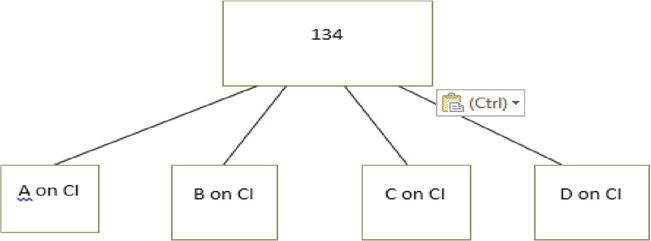
Hence, the lower bound of the total cost from the table above = 48 + 30 + 32 + 24 = 134.

Check and see if you can get a feasible solution from this.

Service outlet D assigned to C1 = N48.

Service outlet B assigned to C2 = N30.

Service outlet D assigned to C3 = N32.

Service outlet D assigned to C4 = N24.

From this, a feasible solution is not attained because service outlet D has been assigned to three different cities while A and C have not been assigned at all.

Therefore we have to proceed by finding a better assignment which entails branching out from our lower bound cost of 134 (see Figure 1).

Figure 1.

Lower bound.

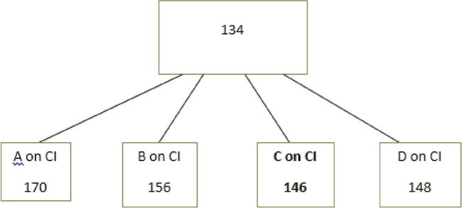
Calculate the cost of assigning jobs to C1.

Assignment to C1

If Service outlet A is assigned to C1 == 84 + 30 + 32 + 24 = 170.

If Job B is assigned to C1 === 60 + 40 + 32 + 24 = 156.

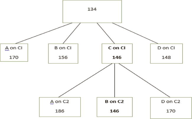
If Job C is assigned to C1 === 60 + 30 + 32 + 24 = 146.

If Job D is assigned to C1 === 48+ 30 + 40 + 30 = 148.

From the assignment above the least cost of assignment is 146 so we assign Service Outlet C to C1 (see Figure 2).

Figure 2.

Assignment of service outlet C to city 1.

Allocate each of the remaining service outlets to C2 to determine the most optimal.

Assignment to C2

If Service outlet A is on C2 ⇒ (60) + 70 + 32 + 24 = 186.

If Service outlet B is on C2 ⇒ (60) + 30 + 32 + 24 = 146.

If Service outlet D is on C2 ⇒ (60) + 40 + 40 + 30 = 170.

The least cost of assignment to C2 is 146, therefore we assign Service Outlet B to City 2 (see Figure 3).

Figure 3.

Assignment of service outlet B to city 2.

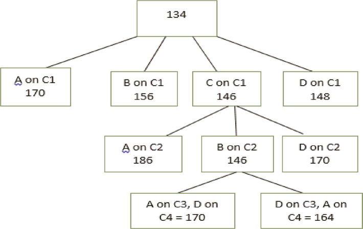
At this point only two cities are left C3 and C4 we can either put service outlet A on C3 and service outlet D on C4 or we can put service outlet A on C3 and A on C4. We obtain the lower bound cost for these remaining assignments as shown below. Note that service outlets C and B are already on C1 and C2 respectively.

Assignment of Service outlets to C3 & C4

Put Service outlet A on C3 and Service outlet D on C4 ⇒ (60 + 30) + 56 + 24 = 170.

Put Service outlet D on C3 and Service outlet A on C4 ⇒ (60 + 30) + 32 + 42 = 164.

Service outlet D is assigned to C3 and Service outlet A to C2.

(See Figure 4).

Assignment	Total
Assign Service outlet C to City 1	60,000
Assign Service outlet B to City 2	30,000
Assign Service outlet D to City 3	32,000
Assign Service outlet A to City 4	42,000
Total Cost	164,000

Figure 4.

Assignment of service outlets a and C.

Hence the optimal assignment of Service Outlets to Cities is as shown above.

Example 2

Suppose as an operations manager, the cost matrix shown above is given to you and you are required to assign the four jobs to the machines in an optional manner using the Branch and Bound method (see Table 37).

Jobs/Machine	1	2	3	4
A	28	42	21	35
B	20	30	12	25
C	16	30	15	25
D	20	24	15	20

Table 37.

Cost matrix.

Solution.

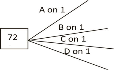
Calculate for lower bound for the total cost of the assignment.

Lower bound cost = 16 + 24 + 12 + 20 = 72.

Job C is best assigned to machine 1.

Job D is best assigned to machine 2.

Job B is best assigned to machine 3.

Job D is best assigned to machine 4.

From this calculation job A is left unassigned to any machine while job D has been assigned to two machines, this is not a feasible assignment because there are multiple assignments of job D. We proceed by branching off from this lower bound cost to determine the best assignment for each machine.

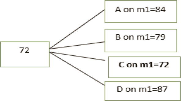
Start by allocating each job in turn to machine 1 to determine the best assignment for machine 1.

Assignment on m1

(See Figure 5).

Figure 5.

Lower bound.

Put A on 1 = 28 + 24 + 12 + 20 = 84.

Put B on 1 = 20 + 24 + 12 + 20 = 79.

Put C on 1 = 16 + 24 + 12 + 20 = 72.

Put D on 1 = 20 + 30 + 12 + 25 = 87.

Therefore Job C is best assignment to machine 1.

(See Figure 6).

Figure 6.

Assignment of job C to machine 1.

Assignment on m₂

Job A on m₂ = (16) + 42 + 12 + 20 = 90.

Job B on m₂ = (16) + 30 + 15 + 20 = 81.

Job D on m₂ = (16) + 24 + 12 + 25 = 77.

(See Figure 7).

Figure 7.

Assignment of job D to machine 2.

Having the lowest cost of 77, job D is best assigned to m2.

Assignment on m3 and m4

Job A on 3, B on 4 = (16 + 24) + 21 + 25 = 86.

Job B on 3, A on 4 = (16 + 24) + 12 + 35 = 87.

(See Figure 8).

Figure 8.

Assignment of job a and B.

Put job A on m3 and job B on m4.

Hence, the optional assignment of the four jobs to machine that will result in the least cost assignment is as follows.

Assign job C to machine 1 = 16.

Assign job D to machine 2 = 24.

Assign job A to machine 3 = 21.

Assign job B to machine 4 = 25.

Total = 86.

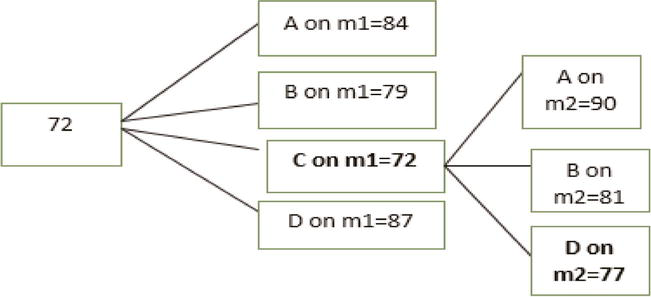
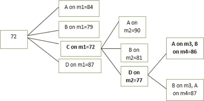
3. Suncity a mobile phone company wishes to allocate its critical tasks to its best four operators and the cost of assigning each task to a particular operator has been provided in the table below, as the company’s operations manager, advice the company on the best assignment that will maximize its total profit.

(See Table 38).

Task/Operators	1	2	3	4
A	130	190	280	200
B	280	310	300	150
C	170	200	210	400
D	120	260	280	210

Table 38.

Profit matrix.

Solution.

In a maximization situation the higher bound of the given matrix is calculated by adding the highest value in each column, from this value we can then branch off to determine the most feasible assignment. It can be observed that all the subsequent profit values after the higher bound is obtained are either equal to, or lower than the higher bound.

Higher bound = 280 + 310 + 300 + 400 = 1290.

The initial assignment will be.

Assign task B to Operator 1.

Assign task B to Operator 2.

Assign task B to Operator 3.

Assign task C to Operator 4.

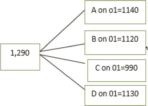
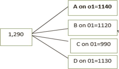
This is not a feasible assignment because we have task B assigned to operator 1, 2 and 3, task C to operator 4, while task A and D have not been assigned to any operator. Hence we branch off from the highest bound to determine the optimal assignment to each operator (see Figure 9).

Figure 9.

Lower bound.

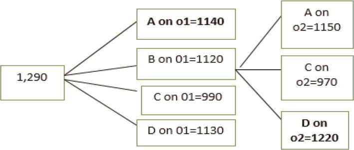
Assignment of task to Operator 1

Assign task A to operator 1 = = 130 + 310 + 300 + 400 = 1140.

Assign task B to operator 1 = = 280 + 260 + 280 + 400 = 1220.

Assign task C to operator 1 = = 170 + 310 + 300 + 210 = 990.

Assign task D to operator 1 = = 120 + 310 + 300 + 400 = 1130.

Therefore, we will assign task B to operator 1 because it yields the highest profit of 1220 (see Figure 10).

Figure 10.

Assignment of task B to operator 1.

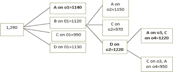
Assignment of task to operator 2

Assign task A to operator 2 = = (280) + 190 + 280 + 400 = 1150.

Assign task C to operator 2 = = (280) + 200 + 280 + 210 = 970.

Assign task D to operator 2 = = (280) + 260 + 280 + 400 = 1220.

Therefore assign task D to operator 2 (see Figure 11).

Figure 11.

Assignment of task D to operator 2.

Assignment of task to operator 3 and 4

Assign task A to operator 3 and task C to operator 4 = (280 + 260) + 280 + 400 = 1220.

Assign task C to operator 3 and task A to operator 4 = (280 + 260) + 210 + 200 = 950.

Hence we assign task A to operator 3 and task C to operator 4 (see Figure 12 and Table 39).

Figure 12.

Assignment of task a and C to operator 3 and 4 respectively.

Optimal Assignment of Task to Operator	Profit
Assign task B to operator 1	280
Assign task D to operator 2	260
Assign task A to operator 3	280
Assign task C to operator 4	400
Total Profit	1220

Table 39.

Assignment table.

7. Conclusion

Facility location is an important aspect of production and operations management. Where to locate a new plant or facility is an expensive decision that is not frequently made. Therefore, caution must be made not to site facilities in non-attractive or less optimal locations, as this will affect the efficiency levels of the production and distribution system of any organization, and in-turn its survival. In determining an optimal facility location, it is observed that the least cost or highest profit may not always be feasible, this is because in real life situations, there are some limitations to choosing the most appropriate allocation. Due to such challenges, there may be need for trade-offs. Hence, the optimal assignment represents the most feasible situation where all the facilities have been suitably assigned locations. The Hungarian and branch and bound method are most suitable approaches to solving location problems.

Practice Questions

1. Given the cost matrix show below, you are required to assign the four Engineers to the four sites in an optimal manner using branch and bound method of liner assignment (see Table 40).

2. Given the profit matrix below assign the operators to the machines in such a way that will maximize the total profit (see Table 41).

Machine/ Jobs	1	2	3	4
A	28	41	18	15
B	42	31	32	38
C	7	41	40	50
D	58	35	19	16

Table 40.

Cost matrix.

Machine/ Jobs	1	2	3	4
A	100	130	150	180
B	140	140	180	100
C	170	80	70	160
D	180	160	110	90

Table 41.

Profit matrix.

Nomenclature list

M	denotes rows
N	denotes columns
//	number of straight lines drawn on a matrix
=	equal to
≠	not equal to