Performance Measurement Using Deterministic and Stochastic Multiplicative Directional Distance Functions

Abstract

Performance measurement is essential for fostering continuous improvement of the production and operation management in a firm or organization. We consider a deterministic scenario based on a flexible structure of production technology and establish a multiplicative relationship between the generalized multiplicative directional distance function (GMDDF) and geometric distance function (GDF). We also introduce a stochastic multiplicative directional distance function (SMDDF). Based on a stochastic scenario, the SMDDF can be estimated by the method of convex nonparametric least squares. As an illustrative application, we investigate the productive performance of Japanese life insurance companies using a panel dataset spanning 2016 to 2020.

1. Introduction

The purpose of this study is to establish the relationship between the generalized multiplicative directional distance function (GMDDF, [1]) and the geometric distance function (GDF, [2]), and to develop a stochastic multiplicative directional distance function (SMDDF) for performance measurement. The GMDDF and GDF are commonly measured by data envelopment analysis (DEA, [3]), a deterministic nonparametric method applicable to multiple-input and multiple-output production technologies. Although the GMDDF and GDF have a multiplicative nature, the original GDF is measured based on a convex production possibility set, whereas the GMDDF is developed with a non-convex production possibility set. From a practical perspective, the convexity assumption may be strong if significant degrees of increasing returns exist. To address a flexible structure of production technology, previous studies in DEA also studied a non-convex production possibility set based on a geometric convexity assumption [1, 4]. The methodology of this study is based on a geometric convex production possibility set, which implicitly models a piecewise log-linear technology. Moreover, it is well known that a one-to-one correspondence relationship exists between the piecewise log-linear technology and the conventional piecewise linear technology. This makes it possible to apply the conventional DEA methods to approach the multiplicative models developed for a geometric convex production possibility set. Therefore, measuring the multiplicative type distance functions is of practical and theoretical interest.

It is also well known that DEA commonly discounts stochastic noise, suggesting that any deviations from the frontier (e.g., gauging the distance to the boundary of the production technology) can be considered a measure of pure inefficiency. By contrast, stochastic frontier analysis (SFA, [5]), a general stochastic parametric approach, accounts for stochastic noise by treating all deviations from the frontier as aggregations of both inefficiency and noise. However, compared with the flexibility of nonparametric measurements, because SFA is a parametric methodology, it relies heavily on an accurately prespecified functional form for production technology. Recently, stochastic nonparametric envelopment of data (StoNED) has been introduced in the literature on efficiency analysis. The StoNED approach relies on the method of convex nonparametric least squares (CNLS), which is a nonparametric regression technique [6]. Both SFA and StoNED are based on a convex production possibility set. This study introduces a stochastic multiplicative directional distance function (SMDDF) based on the geometric convex production possibility set and further proposes an estimation model using CNLS.

The methodology of this study consists of two basic scenarios: deterministic and stochastic. These are performed simultaneously to analyze the productive performance of Japanese life insurance companies. The application demonstrates the advantage of using a combination of GMDDF/GDF and SMDDF, enabling comprehensive understanding of the Japanese life insurance industry.

2. Preliminaries

Consider a sample of $n$ decision-making unitis (DMUs). Denote ${\mathit{x}}_j={\left(x_{1j},\dots ,{\mathit{x}}_{\mathit{mj}}\right)}^T\in {\mathbb{R}}_{++}^m$ and ${\mathit{y}}_j={\left({\mathit{y}}_{1j},\dots ,{\mathit{y}}_{\mathit{sj}}\right)}^T\in {\mathbb{R}}_{++}^s$ as positive input and output vectors of DMU_j ($j=1,\dots ,n$), respectively. The superscript $\mathrm{T}$ stands for a vector transpose. A production technology that transforms inputs into outputs can be defined by the following production possibility set:

$$P≔\left\{\left(\mathit{x},\mathit{y}\right)\in {\mathbb{R}}_{++}^m\times {\mathbb{R}}_{++}^s|\mathit{x}\mathrm{can}\text{produce}\mathit{y}\right\},$$

where $P$ contains the input and output vectors $\left({\mathit{x}}_j,{\mathit{y}}_j\right)$ for all $j=1,\dots ,n$. The conventional DEA-based production technology assumes that $P$ is a closed, bounded, and convex set that satisfies free disposability (see, e.g., [7, 8]). In particular, the ordinary convexity assumption, which is described as below,

$$\begin{array}{l}\left[A1\right]\text{If}\left({\mathit{x}}_1,{\mathit{y}}_1\right)\in P\text{and}\left({\mathit{x}}_2,{\mathit{y}}_2\right)\in P,\text{then}\left(\lambda {\mathit{x}}_1+\left(1-\lambda \right){\mathit{x}}_2,\lambda {\mathit{y}}_1+\left(1-\lambda \right){\mathit{y}}_2\right)\in P\\ \text{for}\mathrm{all}\lambda \in \left[0,1\right]\end{array}$$

requires the marginal products to be nonincreasing. However, this cannot be used to understand productive performances characterized by significant degrees of increasing returns so that the marginal products of inputs may be low with a small-scale economy and may increase sharply as the scale expands beyond a threshold (see, e.g., [9]). To allow a flexible structure of production technology, previous studies [1, 4] postulated a geometric convexity assumption, as below:

$$\begin{array}{l}\left[A{1}^{\prime }\right]\text{If}\left({\mathit{x}}_1,{\mathit{y}}_1\right)\in P\text{and}\left({\mathit{x}}_2,{\mathit{y}}_2\right)\in P,\text{then}{\left({\mathit{x}}_1,{\mathit{y}}_1\right)}^{\lambda }\otimes {\left({\mathit{x}}_2,{\mathit{y}}_2\right)}^{1-\lambda }\in P\\ \text{for}\mathrm{all}\lambda \in \left[0,1\right],\end{array}$$

where $\otimes$ stands for the element-wise multiplication of vectors. By replacing $A1$ with $A{1}^{\prime }$, $P$ is not restricted to be concave (e.g., the underlying production function can be S-shaped) and is capable of capturing the potential existence of increasing, constant, or decreasing marginal products. For empirical studies that use a non-concave production technology, see [10, 11], among others.

In this study, we proceed with the performance measurement using $P$ that satisfies closedness, boundedness, geometric convexity, and free disposability. Based on a given $P$, the generalized multiplicative directional distance function (GMDDF, [1]) is defined as

$$M\left(\mathit{x},\mathit{y};-{\mathit{g}}^{-},{\mathit{g}}^{+}\right)≔sup\left\{{\left(\prod _{i=1}^m{\alpha }_i\right)}^{\frac{1}{m}}\times {\left(\prod _{r=1}^s{\beta }_r\right)}^{\frac{1}{r}}\left|\left({\mathit{\alpha }}^{-{\mathit{g}}^{-}}\mathit{x},{\mathit{\beta }}^{{\mathbf{g}}^{+}}\mathit{y}\right)\in P,\mathit{\alpha }\ge {\mathbf{1}}_m,\mathit{\beta }\ge {\mathbf{1}}_s\right.\right\},$$E1

where $\mathit{g}≔\left(-{\mathit{g}}^{-},{\mathit{g}}^{+}\right)\in \left(-{\mathbb{R}}_{+}^m\right)\times {\mathbb{R}}_{+}^s$ is a prespecified direction vector and

$${\mathit{\alpha }}^{-{\mathit{g}}^{-}}≔\left[\begin{array}{ccc}{\alpha }_1^{-g_1^{-}}& \cdots & 0\\ ⋮& \ddots & ⋮\\ 0& \cdots & {\alpha }_m^{-g_m^{-}}\end{array}\right]\text{and}{\mathit{\beta }}^{{\mathit{g}}^{+}}≔\left[\begin{array}{ccc}{\beta }_1^{g_1^{+}}& \cdots & 0\\ ⋮& \ddots & ⋮\\ 0& \cdots & {\beta }_s^{g_s^{+}}\end{array}\right].$$

According to definition (1), both inputs and outputs are changed simultaneously along with a given direction $\mathit{g}$ and are eventually projected onto the frontier (boundary) of $P$. Denote the points on the frontier of $P$ as $\left({\mathit{x}}^{\ast },{\mathit{y}}^{\ast }\right)$. We hereby list the main properties of $M\left(\mathit{x},\mathit{y};-{\mathit{g}}^{-},{\mathit{g}}^{+}\right)$ used in this study, as below (See [1] for details on the proofs):

P1: $M\left(\mathit{x},\mathit{y};-{\mathit{g}}^{-},{\mathit{g}}^{+}\right)\ge 1$ if and only if $\left(\mathit{x},\mathit{y}\right)\in P$.

P2: $M\left({\mathit{x}}^{\ast },{\mathit{y}}^{\ast };-{\mathit{g}}^{-},{\mathit{g}}^{+}\right)=1$ for any given $\left(-{\mathit{g}}^{-},{\mathit{g}}^{+}\right)\in \left(-{\mathbb{R}}_{+}^m\right)\times {\mathbb{R}}_{+}^s$.

P3: $logM\left(\mathit{x},\mathit{y};-{\mathit{g}}^{-},{\mathit{g}}^{+}\right)$ is concave on $logP$,

where $logP≔\left\{\left(log\mathit{x},log\mathit{y}\right)\in {\mathbb{R}}^m\times {\mathbb{R}}^s|(\mathit{x},\mathit{y})\in P\right\}$.

The property P1 means that $M\left(\mathit{x},\mathit{y};-{\mathit{g}}^{-},{\mathit{g}}^{+}\right)$ is a functional representation of $P$, that is

$$P=\left\{\left(\mathit{x},\mathit{y}\right)\in {\mathbb{R}}_{++}^m\times {\mathbb{R}}_{++}^s|M\left(\mathit{x},\mathit{y};-{\mathit{g}}^{-},{\mathit{g}}^{+}\right)\ge 1\right\}\text{for}\mathrm{any}\text{given}\left(-{\mathit{g}}^{-},{\mathit{g}}^{+}\right)\in \left(-{\mathbb{R}}_{+}^m\right)\times {\mathbb{R}}_{+}^s.$$

We first consider a deterministic scenario, in which all producible input-output vectors are only affected by inefficiencies.

Proposition 1.1. Let ${\delta }_{x_i}\le 1$ for all $i=1,\dots ,m$ and ${\delta }_{y_r}\ge 1$ for all $r=1,\dots ,s$. Assume that a projection point $\left({\mathit{x}}^{\ast },{\mathit{y}}^{\ast }\right)$ for the DMU $\left(\mathit{x},\mathit{y}\right)$ is achieved by improving $\left(\mathit{x},\mathit{y}\right)$ at exponential changes of a vector $\left({\mathit{\delta }}_{\mathit{x}},\frac{1}{{\mathit{\delta }}_{\mathit{y}}}\right)$ by the power of a given vector $\left({\mathit{g}}^{-},-{\mathit{g}}^{+}\right)\in {\mathbb{R}}_{+}^m\times \left(-{\mathbb{R}}_{+}^s\right)$. Specifically,

$$\left({\mathit{x}}^{\ast },{\mathit{y}}^{\ast }\right)=\left({\mathit{\delta }}_{\mathit{x}}^{{\mathit{g}}^{-}}\mathit{x},{\left(\frac{\mathrm{1}}{{\mathit{\delta }}_y}\right)}^{-{\mathit{g}}^{+}}\mathit{y}\right),$$E2

where

$${\mathit{\delta }}_{\mathit{x}}^{{\mathit{g}}^{-}}≔\left[\begin{array}{ccc}{\delta }_{x_1}^{g_1^{-}}& \cdots & 0\\ ⋮& \ddots & ⋮\\ 0& \cdots & {\delta }_{x_m}^{g_m^{-}}\end{array}\right]\text{and}{\left(\frac{1}{{\mathit{\delta }}_{\mathit{y}}}\right)}^{-{\mathit{g}}^{+}}≔\left[\begin{array}{ccc}{\left(\frac{1}{{\delta }_{y_1}}\right)}^{-g_1^{+}}& \cdots & 0\\ ⋮& \ddots & ⋮\\ 0& \cdots & {\left(\frac{1}{{\delta }_{y_s}}\right)}^{-g_s^{+}}\end{array}\right].$$

Then, the value of $M\left(\mathit{x},\mathit{y};-{\mathit{g}}^{-},{\mathit{g}}^{+}\right)$ for the observed DMU $\left(\mathit{x},\mathit{y}\right)$ satisifies

$$M\left(\mathit{x},\mathit{y};-{\mathit{g}}^{-},{\mathit{g}}^{+}\right)=u,$$E3

where

$$u≔{\left(\prod _{i=1}^m\frac{1}{{\delta }_{x_i}}\right)}^{\frac{1}{m}}{\left(\prod _{r=1}^s{\delta }_{y_r}\right)}^{\frac{1}{s}}.$$E4

Proof: According to the definition (1), we have

$$\begin{array}{l}\mathit{M}\left({\mathit{\delta }}_{\mathit{x}}^{{\mathit{g}}^{-}}\mathit{x},{\left(\frac{1}{{\mathit{\delta }}_{\mathit{y}}}\right)}^{-{\mathit{g}}^{+}}\mathit{y};-{\mathit{g}}^{-},{\mathit{g}}^{+}\right)\\ =\begin{array}{l}sup\{{\left(\prod _{i=1}^m{\alpha }_i\right)}^{\frac{1}{m}}\times {\left(\prod _{r=1}^s{\beta }_r\right)}^{\frac{1}{r}}|\left({\mathit{\alpha }}^{-{\mathit{g}}^{-}}\otimes {\mathit{\delta }}_{\mathit{x}}^{{\mathit{g}}^{-}}\mathit{x},{\mathit{\beta }}^{{\mathit{g}}^{+}}\otimes {\left(\frac{1}{{\mathit{\delta }}_{\mathit{y}}}\right)}^{-{\mathit{g}}^{+}}\mathit{y}\right)\in P,\mathit{\alpha }\ge {\mathbf{1}}_{\mathit{m}},\mathit{\beta }\ge {\mathbf{1}}_{\mathit{s}}\}\end{array}\\ =\begin{array}{l}{\left(\prod _{i=1}^m{\delta }_{x_i}\right)}^{\frac{1}{m}}{\left(\prod _{r=1}^s\frac{1}{{\delta }_{y_r}}\right)}^{\frac{1}{s}}sup\{{\left(\prod _{i=1}^m\frac{{\alpha }_i}{{\delta }_{x_i}}\right)}^{\frac{1}{m}}\times {\left(\prod _{r=1}^s{\beta }_r{\delta }_{y_r}\right)}^{\frac{1}{r}}\left|\begin{array}{l}\left({\mathit{\alpha }}^{-{\mathit{g}}^{-}}\otimes {\mathit{\delta }}_{\mathit{x}}^{{\mathit{g}}^{-}}\mathit{x},{\mathit{\beta }}^{{\mathbf{g}}^{+}}\otimes {\left(\frac{1}{{\mathit{\delta }}_{\mathit{y}}}\right)}^{-{\mathit{g}}^{+}}\mathit{y}\right)\in P,\\ \mathit{\alpha }\oslash {\mathit{\delta }}_{\mathit{x}}\ge {\mathbf{1}}_{\mathit{m}},\mathit{\beta }\otimes {\mathit{\delta }}_{\mathit{y}}\ge {\mathbf{1}}_{\mathit{s}}\end{array}\right\}\end{array}\\ ={\left(\prod _{i=1}^m{\delta }_{x_i}\right)}^{\frac{1}{m}}{\left(\prod _{r=1}^s\frac{1}{{\delta }_{y_r}}\right)}^{\frac{1}{s}}\mathit{M}\left(\mathit{x},\mathit{y};-{\mathit{g}}^{-},{\mathit{g}}^{+}\right).\end{array}$$

Note that $\oslash$ denotes the element-wise division of vectors. Due to the assumption (2), we obtain

$$\begin{array}{c}\mathit{M}\left({\mathit{x}}^{\ast },{\mathit{y}}^{\ast };-{\mathit{g}}^{-},{\mathit{g}}^{+}\right)=\mathit{M}\left({\mathit{\delta }}_{\mathit{x}}^{{\mathit{g}}^{-}}\mathit{x},{\left(\frac{\mathbf{1}}{{\mathit{\delta }}_{\mathit{y}}}\right)}^{-{\mathit{g}}^{+}}\mathit{y};-{\mathit{g}}^{-},{\mathit{g}}^{+}\right)\\ ={\left(\prod _{\mathit{i}=1}^m{\delta }_{x_i}\right)}^{\frac{1}{m}}{\left(\prod _{r=1}^s\frac{1}{{\delta }_{y_r}}\right)}^{\frac{1}{s}}\mathit{M}\left(\mathit{x},\mathit{y};-{\mathit{g}}^{-},{\mathit{g}}^{+}\right).\end{array}$$

Because of P2, we obtain

$$\mathit{M}\left(\mathit{x},\mathit{y};-{\mathit{g}}^{-},{\mathit{g}}^{+}\right)={\left(\prod _{i=1}^m\frac{1}{{\delta }_{x_i}}\right)}^{\frac{1}{m}}{\left(\prod _{r=1}^s{\delta }_{y_r}\right)}^{\frac{1}{s}}.$$

It is worthnoting that Eq. (4) is equal to the reciprocal of the geometric distance function (GDF) introduced by [2]:

$$\varphi ≔{\left(\prod _{i=1}^m{\delta }_{x_i}\right)}^{\frac{1}{m}}{\left(\prod _{r=1}^s\frac{1}{{\delta }_{y_r}}\right)}^{\frac{1}{s}},$$

which is a non-oriented efficiency measure that incorporates both input contraction and output expansion toward the projection points. Note that the original GDF is developed based on the ordinary convexity assumption. However, it is possible to reformulate the GDF on a given $P$ (that satisfies geometric convexity). In such a case, the GDF can be considered a specific case of the GMDDF with $\left(-{\mathit{g}}^{-},{\mathit{g}}^{+}\right)=\left(-{\mathbf{1}}_m,{\mathbf{1}}_s\right)$, that is, $M\left(\mathit{x},\mathit{y};-{\mathbf{1}}_m,{\mathbf{1}}_s\right)$. In the scenario described in Proposition 1, the relationship between the GMDDF and GDF can be stated as

$$\begin{array}{c}\mathit{M}\left({\mathit{x}}^{\ast },{\mathit{y}}^{\ast };-{\mathit{g}}^{-},{\mathit{g}}^{+}\right)=\mathit{M}\left(\mathit{x},\mathit{y};-{\mathbf{1}}_{\mathit{m}},{\mathbf{1}}_{\mathit{s}}\right)\times \mathit{M}\left(\mathit{x},\mathit{y};-{\mathit{g}}^{-},{\mathit{g}}^{+}\right)\\ =\mathit{\varphi }\times \mathit{M}\left(\mathit{x},\mathit{y};-{\mathit{g}}^{-},{\mathit{g}}^{+}\right).\end{array}$$

Consequently, $u\left(=1/\varphi \right)$ can be used as an inefficiency measure with a range of $\left[1,\infty \right)$.

3. A stochastic multiplicative directional distance function

In this section, we further consider a stochastic scenario in which all observations (i.e., $\left({\mathit{x}}_j,{\mathit{y}}_j\right),\forall j=1,\dots ,n$) in $P$ are random variables and have their unique deterministic projection point (efficient point) on the frontier of $P$ (i.e., $\left({\mathit{x}}_j^{\ast },{\mathit{y}}_j^{\ast }\right),\forall j=1,\dots ,n$). We assume that the difference between the observation point and the projection point is not only caused by the inefficiency term but also by random noise. Since the generalized multiplicative directional distance function ranges from 1 to $\infty$, it does not have a straightforward representation to describe the stochastic setting. Therefore, we introduce a stochatsic multiplicative directional distance function (SMDDF), which is defined as follows:

$$\tilde{\mathit{M}}\left(\mathit{x},\mathit{y};-{\mathit{g}}^{-},{\mathit{g}}^{+}\right)≔sup\left\{{\left(\prod _{i=1}^m{\alpha }_i\right)}^{\frac{1}{m}}\times {\left(\prod _{r=1}^s{\beta }_r\right)}^{\frac{1}{r}}\left|\left({\mathit{\alpha }}^{-{\mathbf{g}}^{-}}\mathit{x},{\mathit{\beta }}^{{\mathit{g}}^{+}}\mathit{y}\right)\in \mathit{P},\mathit{\alpha }>{\mathbf{0}}_{\mathit{m}},\mathit{\beta }>{\mathbf{0}}_{\mathit{s}}\right.\right\},$$E5

where $\mathit{x}$ and $\mathit{y}$ are random variables.

Some properties of $\tilde{M}\left(\mathit{x},\mathit{y};-{\mathit{g}}^{-},{\mathit{g}}^{+}\right)$ are described as below:

P1’: $\tilde{M}\left(\mathit{x},\mathit{y};-{\mathit{g}}^{-},{\mathit{g}}^{+}\right)>0$ if and only if $\left(\mathit{x},\mathit{y}\right)\in P$.

P2’: $\tilde{M}\left({\mathit{x}}^{\ast },{\mathit{y}}^{\ast };-{\mathit{g}}^{-},{\mathit{g}}^{+}\right)=1$ for any given $\left(-{\mathit{g}}^{-},{\mathit{g}}^{+}\right)\in \left(-{\mathbb{R}}_{+}^m\right)\times {\mathbb{R}}_{+}^s$.

P3’: $log\tilde{M}\left(\mathit{x},\mathit{y};-{\mathit{g}}^{-},{\mathit{g}}^{+}\right)$ is concave on $logP$,

where $logP≔\left\{\left(log\mathit{x},log\mathit{y}\right)\in {\mathbb{R}}^m\times {\mathbb{R}}^s|(\mathit{x},\mathit{y})\in P\right\}$.

The property P1’ is evident from the definition (5). P2’ holds because the frontier containing all of the projection points $\left({\mathit{x}}^{\ast },{\mathit{y}}^{\ast }\right)$ is assumed to be deterministic. P3’ can be proved in a similar way with P3 (see [1] for further details). Furthermore, $\tilde{M}\left(\mathit{x},\mathit{y};-{\mathit{g}}^{-},{\mathit{g}}^{+}\right)$ has the following translation property:

Proposition 1.2. For any positive vector $\left(\mathit{\theta },\mathit{\eta }\right)\in {\mathbb{R}}_{++}^{m+s}$,

$$log\tilde{M}\left({\mathit{\theta }}^{-{\mathit{g}}^{-}}\mathit{x},{\mathit{\eta }}^{{\mathit{g}}^{+}}\mathit{y};-{\mathit{g}}^{-},{\mathit{g}}^{+}\right)=log\tilde{M}\left(\mathit{x},\mathit{y};-{\mathit{g}}^{-},{\mathit{g}}^{+}\right)-\left(\frac{1}{m}\sum _{i=1}^{m}log{\theta }_i+\frac{1}{s}\sum _{r=1}^{s}log{\eta }_r\right)$$

holds.

Proof: From the definition (5), we obtain

$$\begin{array}{l}log\tilde{M}\left(\mathit{x},\mathit{y};-{\mathit{g}}^{-},{\mathit{g}}^{+}\right)=log\left(sup\left\{{\left(\prod _{i=1}^m{\alpha }_i\right)}^{\frac{1}{m}}\times {\left(\prod _{r=1}^s{\beta }_r\right)}^{\frac{1}{r}}\left|\begin{array}{l}\left({\mathit{\alpha }}^{-{\mathbf{g}}^{-}}\mathit{x},{\mathit{\beta }}^{{\mathit{g}}^{+}}\mathit{y}\right)\in P,\\ \mathit{\alpha }>{\mathbf{0}}_{\mathit{m}},\mathit{\beta }>{\mathbf{0}}_{\mathit{s}}\end{array}\right.\right\}\right)\\ =sup\left\{\frac{1}{m}\sum _{i=1}^{m}log{\alpha }_i+\frac{1}{s}\sum _{r=1}^{s}log{\beta }_r\left|\begin{array}{l}\left(log\mathit{x}\mathbf{-}{\mathit{g}}^{\mathbf{-}}\otimes log\mathit{\alpha },log\mathit{y}\mathbf{+}{\mathit{g}}^{\mathbf{+}}\otimes log\mathit{\beta }\right)\in logP,\\ log\mathit{\alpha }:\text{free},log\mathit{\beta }:\text{free}\end{array}\right.\right\}.\end{array}$$

Therefore, for any positive vector $\left(\mathit{\theta },\mathit{\eta }\right)\in {\mathbb{R}}_{++}^{m+s}$, we obtain

$$\begin{array}{l}log\tilde{M}\left({\mathit{\theta }}^{-{\mathit{g}}^{-}}\mathit{x},{\mathit{\eta }}^{{\mathit{g}}^{+}}\mathit{y};-{\mathit{g}}^{-},{\mathit{g}}^{+}\right)=sup\left\{\frac{1}{m}\sum _{i=1}^{m}log{\alpha }_i+\frac{1}{s}\sum _{r=1}^{s}log{\beta }_r,\right.\\ \left(log\mathit{x}\mathbf{-}{\mathit{g}}^{\mathbf{-}}\otimes log\mathit{\theta }\mathbf{-}{\mathit{g}}^{\mathbf{-}}\otimes log\mathit{\alpha },log\mathit{y}\mathbf{+}{\mathit{g}}^{\mathbf{+}}\otimes log\mathit{\eta }\mathbf{+}{\mathit{g}}^{\mathbf{+}}\otimes log\mathit{\beta }\right)\in logP,\\ log\mathit{\alpha }:\text{free},log\mathit{\beta }:\text{free}\\ =-\left(\frac{1}{m}\sum _{i=1}^{m}log{\theta }_i+\frac{1}{s}\sum _{r=1}^{s}log{\eta }_r\right)\\ \left.+sup\left\{\frac{1}{m}\sum _{i=1}^{m}log{\alpha }_i+\frac{1}{s}\sum _{r=1}^{s}log{\beta }_r+\left(\frac{1}{m}\sum _{i=1}^{m}log{\theta }_i+\frac{1}{s}\sum _{r=1}^{s}log{\eta }_r\right)\right.\right|\\ \left.\begin{array}{l}\left(log\mathit{x}\mathbf{-}{\mathit{g}}^{\mathbf{-}}\otimes \left(log\mathit{\alpha }\mathbf{+}log\mathit{\theta }\right),log\mathit{y}\mathbf{+}{\mathit{g}}^{\mathbf{+}}\otimes \left(log\mathit{\beta }\mathbf{+}log\mathit{\eta }\right)\right)\in logP,\\ log\mathit{\alpha }\mathbf{+}log\mathit{\theta }:\text{free},log\mathit{\beta }+log\mathit{\eta }:\text{free}\end{array}\right\}\\ =log\tilde{M}\left(\mathit{x},\mathit{y};\mathbf{-}{\mathit{g}}^{\mathbf{-}},{\mathit{g}}^{\mathbf{+}}\right)-\left(\frac{1}{m}\sum _{i=1}^{m}log{\theta }_i+\frac{1}{s}\sum _{r=1}^{s}log{\eta }_r\right).\end{array}$$

It is worth noting that the proposed $\tilde{M}\left(\mathit{x},\mathit{y};-{\mathit{g}}^{-},{\mathit{g}}^{+}\right)$ precisely reveals a multiplicative data-generating process. To help inform intuition regarding this type of data-generating process, let ${ϵ}_{x_i}>0$ for all $i=1,\dots ,m$ and ${ϵ}_{y_r}>0$ for all $r=1,\dots ,s$ be the element-specific composite errors for inputs and outputs, respectively. Since $\mathit{x}$ and $\mathit{y}$ are random variables that are subject to both inefficiencies and noises, we assume that $E\left({ϵ}_{x_i}\right)={\mu }_{x_i}>0$, $\mathit{Var}\left({ϵ}_{x_i}\right)<\infty$ and $E\left({ϵ}_{y_i}\right)={\mu }_{y_i}>0$, $\mathit{Var}\left({ϵ}_{y_i}\right)<\infty$. Suppose that

$$\left(\mathit{x},\mathit{y}\right)=\left({\mathit{ϵ}}_{\mathit{x}}^{{\mathit{g}}^{-}}{\mathit{x}}^{\ast },{\mathit{ϵ}}_{\mathit{y}}^{-{\mathit{g}}^{+}}{\mathit{y}}^{\ast }\right).$$E6

Then, it follows from Proposition 1.2 and property P2’ that

$$log\tilde{M}\left(\mathit{x},\mathit{y};-{\mathit{g}}^{-},{\mathit{g}}^{+}\right)=\frac{1}{\mathit{m}}\sum _{\mathit{i}=1}^{\mathit{m}}log{\mathit{ϵ}}_{{\mathit{x}}_{\mathit{i}}}+\frac{1}{\mathit{s}}\sum _{\mathit{r}=1}^{\mathit{s}}log{\mathit{ϵ}}_{{\mathit{y}}_{\mathit{r}}},$$E7

which is equivalent to

$$\tilde{M}\left(\mathit{x},\mathit{y};-{\mathit{g}}^{-},{\mathit{g}}^{+}\right)={\left(\prod _{\mathit{i}=1}^{\mathit{m}}{\mathit{ϵ}}_{{\mathit{x}}_{\mathit{i}}}\right)}^{\frac{1}{\mathit{m}}}\times {\left(\prod _{\mathit{r}=1}^{\mathit{s}}{\mathit{ϵ}}_{{\mathit{y}}_{\mathit{r}}}\right)}^{\frac{1}{\mathit{r}}}.$$

To simplify the notation, we define $ϵ≔{\left({\prod }_{i=1}^m{ϵ}_{x_i}\right)}^{\frac{1}{m}}\times {\left({\prod }_{r=1}^s{ϵ}_{y_r}\right)}^{\frac{1}{r}}$. Then,

$$\tilde{M}\left(\mathit{x},\mathit{y};-{\mathit{g}}^{-},{\mathit{g}}^{+}\right)=\mathit{ϵ}.$$

Therefore, $\tilde{M}\left(\mathit{x},\mathit{y};-{\mathit{g}}^{-},{\mathit{g}}^{+}\right)$ can be interpreted as a composite error term that is constructed with ${ϵ}_{x_i}\left(\forall i\right)$ and ${ϵ}_{y_r}\left(\forall r\right)$. Moreover, from the linearity of expectation and Jensen’s inequality, we also have $0<\mu ≔E\left(logϵ\right)=E\left(\frac{1}{m}{\sum }_{i=1}^{m}log{ϵ}_{x_i}+\frac{1}{s}{\sum }_{r=1}^{s}log{ϵ}_{y_r}\right)\le$$\frac{1}{m}{\sum }_{i=1}^{m}log{\mu }_{x_i}+\frac{1}{s}{\sum }_{r=1}^{s}log{\mu }_{y_r}$.

To estimate the inefficiency for the observed DMU${}_j$ ($j=1,\dots ,n$) as well as the SMDDF, we apply Proposition 1.2 and set $\left({\mathit{\theta }}_j,{\mathit{\eta }}_j\right)=\left({\mathit{x}}_j,{\mathit{y}}_j\right)$ to obtain the following equality:

$$log\tilde{M}\left({\mathit{x}}_{\mathit{j}}^{{\mathit{g}}^{-}}{\mathit{x}}_{\mathit{j}},{\mathit{y}}_{\mathit{j}}^{-{\mathit{g}}^{+}}{\mathit{y}}_{\mathit{j}};-{\mathit{g}}^{-},{\mathit{g}}^{+}\right)=log\tilde{M}\left({\mathit{x}}_{\mathit{j}},{\mathit{y}}_{\mathit{j}};-{\mathit{g}}^{-},{\mathit{g}}^{+}\right)+\left(\frac{1}{m}\sum _{i=1}^{m}log{x}_{\mathit{ij}}+\frac{1}{s}\sum _{r=1}^{s}log{y}_{\mathit{rj}}\right).$$

Using Eq. (7), we further obtain

$$\begin{array}{c}\frac{1}{m}\sum _{i=1}^{m}log{x}_{\mathit{ij}}+\frac{1}{s}\sum _{r=1}^{s}log{y}_{\mathit{rj}}=log\tilde{M}\left({\mathit{x}}_{\mathit{j}}^{{\mathit{g}}^{-}}{\mathit{x}}_{\mathit{j}},{\mathit{y}}_{\mathit{j}}^{-{\mathit{g}}^{+}}{\mathit{y}}_{\mathit{j}};-{\mathit{g}}^{-},{\mathit{g}}^{+}\right)-log\tilde{M}\left({\mathit{x}}_{\mathit{j}},{\mathit{y}}_{\mathit{j}};-{\mathit{g}}^{-},{\mathit{g}}^{+}\right)\\ =log\tilde{M}\left({\mathit{x}}_{\mathit{j}}^{{\mathit{g}}^{-}}{\mathit{x}}_{\mathit{j}},{\mathit{y}}_{\mathit{j}}^{-{\mathit{g}}^{+}}{\mathit{y}}_{\mathit{j}};-{\mathit{g}}^{-},{\mathit{g}}^{+}\right)-log{ϵ}_j.\end{array}$$

Let ${\tilde{\mathit{x}}}_j={\left({\mathit{x}}_j\right)}^{{\mathit{g}}^{-}}{\mathit{x}}_j$ and ${\tilde{\mathit{y}}}_j={\left({\mathit{y}}_j\right)}^{-{\mathit{g}}^{+}}{\mathit{y}}_j$. Then,

$$\begin{array}{l}\overline{\overline{M}}\left({\tilde{\mathit{x}}}_{\mathit{j}},{\tilde{\mathit{y}}}_{\mathit{j}};-{\mathit{g}}^{-},{\mathit{g}}^{+}\right)≔E\left(log\tilde{M}\left({\tilde{\mathit{x}}}_{\mathit{j}},{\tilde{\mathit{y}}}_{\mathit{j}};-{\mathit{g}}^{-},{\mathit{g}}^{+}\right)\right)-E\left(log{ϵ}_j\right)\\ =log\tilde{M}\left({\tilde{\mathit{x}}}_{\mathit{j}},{\tilde{\mathit{y}}}_{\mathit{j}};-{\mathit{g}}^{-},{\mathit{g}}^{+}\right)-\mu \end{array}$$

It follows from P3 that $\tilde{M}\left({\tilde{\mathit{x}}}_j,{\tilde{\mathit{y}}}_j;-{\mathit{g}}^{-},{\mathit{g}}^{+}\right)$ is a concave function. Moreover, $\overline{\overline{M}}\left({\tilde{\mathit{x}}}_j,{\tilde{\mathit{y}}}_j;-{\mathit{g}}^{-},{\mathit{g}}^{+}\right)$ could be seen as the conditional expectation function of $\left(\frac{1}{m}{\sum }_{i=1}^{m}log{x}_{\mathit{ij}}+\frac{1}{s}{\sum }_{r=1}^{s}log{y}_{\mathit{rj}}\right)$. That is,

$$\frac{1}{m}\sum _{i=1}^{m}log{x}_{\mathit{ij}}+\frac{1}{s}\sum _{r=1}^{s}log{y}_{\mathit{rj}}=\overline{\overline{M}}\left({\tilde{\mathit{x}}}_{\mathit{j}},{\tilde{\mathit{y}}}_{\mathit{j}};-{\mathit{g}}^{-},{\mathit{g}}^{+}\right)-{\xi }_j,$$

where ${\xi }_j=log{u}_j+v_j-\mu$ and $u_j$ is a DMU-specific inefficiency term that satisfies $E\left(log{u}_j\right)=\mu$, $\mathit{Var}\left(log{u}_j\right)<\infty$, and $v_j$ is a noise term that satisfies $E\left(v_j\right)=0$, $\mathit{Var}\left(v_j\right)<\infty$.

To estimate $\overline{\overline{M}}\left({\tilde{\mathit{x}}}_j,{\tilde{\mathit{y}}}_j;-{\mathit{g}}^{-},{\mathit{g}}^{+}\right)$ as well as the average level of inefficiencies, we apply the method of convex nonparametric least squares (CNLS, [6]), which is a nonparametric regression approach with a least-square objective subject to monotonicity and convexity/concavity constraints. However, the definition of SMDDF requires additional conditions that Proposition 1.2 should hold, contrary to constraints of the ordinary CNLS problem. Therefore, we formulate the CNLS problem as the following quadratic programming (QP) problem:

$$min\sum _{j=1}^n{\xi }_j^2$$E8

$$\mathrm{s}.\mathrm{t}.\frac{1}{m}\sum _{i=1}^{m}log{x}_{\mathit{ij}}+\frac{1}{s}\sum _{r=1}^{s}log{y}_{\mathit{rj}}={\upsilon }_j+\sum _{i=1}^m{\zeta }_{\mathit{ij}}log{\tilde{x}}_{\mathit{ij}}-\sum _{r=1}^s{\gamma }_{\mathit{rj}}log{\tilde{y}}_{\mathit{rj}}-{\xi }_j,\forall j$$E9

$${\upsilon }_j+\sum _{i=1}^m{\zeta }_{\mathit{ij}}log{\tilde{x}}_{\mathit{ij}}-\sum _{r=1}^s{\gamma }_{\mathit{rj}}log{\tilde{y}}_{\mathit{rj}}\le {\upsilon }_h+\sum _{i=1}^m{\zeta }_{\mathit{ih}}log{\tilde{x}}_{\mathit{ij}}-\sum _{r=1}^s{\gamma }_{\mathit{rh}}log{\tilde{y}}_{\mathit{rj}},\forall j,h\text{and}j\ne h$$E10

$$\sum _{i=1}^m{\zeta }_{\mathit{ij}}{g}_{\mathit{ij}}^{-}log{x}_{\mathit{ij}}+\sum _{r=1}^s{\gamma }_{\mathit{rj}}{g}_{\mathit{rj}}^{+}log{y}_{\mathit{rj}}=\frac{1}{m}\sum _{i=1}^{m}log{x}_{\mathit{ij}}+\frac{1}{s}\sum _{r=1}^{s}log{y}_{\mathit{rj}},\forall j$$E11

$${\zeta }_{\mathit{ij}}\ge 0,{\gamma }_{\mathit{rj}}\ge 0,\forall i,r,j.$$E12

The objective function (8) and the constraint (9) fit a linear equation for each DMU_j, where $\frac{1}{m}{\sum }_{i=1}^{m}log{x}_{\mathit{ij}}+\frac{1}{s}{\sum }_{r=1}^{s}log{y}_{\mathit{rj}}$ is the dependent variable and $\left({\tilde{\mathit{x}}}_j,-{\tilde{\mathit{y}}}_j\right)$ is the independent variable. The second constraint (10) further imposes Afrait’s theorem [12], which ensures global concavity of the estimated $\overline{\overline{M}}\left({\tilde{\mathit{x}}}_j,{\tilde{\mathit{y}}}_j;-{\mathit{g}}^{-},{\mathit{g}}^{+}\right)$. The third constraint (11) ensures the translation property as described in Proposition 1.2. The last two constraints in (12) impose monotonicity relative to all transformed inputs ${\tilde{\mathit{x}}}_j$ and outputs ${\tilde{\mathit{y}}}_j$. Using the translation property, the above problem can be reformulated as

$$min\sum _{j=1}^n{\xi }_j^2$$E13

$$\mathrm{s}.\mathrm{t}.\sum _{r=1}^s{\gamma }_{\mathit{rj}}log{y}_{\mathit{rj}}={\upsilon }_j+\sum _{i=1}^m{\zeta }_{\mathit{ij}}log{x}_{\mathit{ij}}-{\xi }_j,\forall j$$E14

$${\upsilon }_j+\sum _{i=1}^m{\zeta }_{\mathit{ij}}log{x}_{\mathit{ij}}-\sum _{r=1}^s{\gamma }_{\mathit{rj}}log{y}_{\mathit{rj}}\le {\upsilon }_h+\sum _{i=1}^m{\zeta }_{\mathit{ih}}log{x}_{\mathit{ij}}-\sum _{r=1}^s{\gamma }_{\mathit{rh}}log{y}_{\mathit{rj}},\forall j,h\text{and}j\ne h$$E15

$$\sum _{i=1}^m{\zeta }_{\mathit{ij}}{g}_{\mathit{ij}}^{-}log{x}_{\mathit{ij}}+\sum _{r=1}^s{\gamma }_{\mathit{rj}}{g}_{\mathit{rj}}^{+}log{y}_{\mathit{rj}}=\frac{1}{m}\sum _{i=1}^{m}log{x}_{\mathit{ij}}+\frac{1}{s}\sum _{r=1}^{s}log{y}_{\mathit{rj}},\forall j$$E16

$${\zeta }_{\mathit{ij}}\ge 0,{\gamma }_{\mathit{rj}}\ge 0,\forall i,r,j,$$E17

where the constraint (14) now is a linear equation of inputs and outputs for each DMU_j. Since the problems (13)–(17) estimate $\overline{\overline{M}}\left({\tilde{\mathit{x}}}_j,{\tilde{\mathit{y}}}_j;-{\mathit{g}}^{-},{\mathit{g}}^{+}\right)$ as a concave function, the coefficients ${\upsilon }_j,{\zeta }_{\mathit{ij}},{\gamma }_{\mathit{rj}},\forall i,r$ characterize a tangent hyperplane of the estimated $\overline{\overline{M}}\left({\tilde{\mathit{x}}}_j,{\tilde{\mathit{y}}}_j;-{\mathit{g}}^{-},{\mathit{g}}^{+}\right)$ for each DMU_j.

After solving the problem (13)–(17), it is possible to derive the expected value of the logarithm of inefficiencies (i.e., $\mu$) based on the skewness of the estimated residuals. For example, $\mu$ can be measured using the method of moments [5] (Note that alternative approaches such as quasi-likelihood estimation and nonparametric kernel deconvolution are available. See, e.g., [13] for a detailed discussion).

4. Application to Japanese life insurance companies

In this section, we investigate the productive performance of Japanese life insurance companies by considering both deterministic and stochastic scenarios. The sample consisted of 41 member companies of the Life Insurance Association of Japan (LIAJ). We considered the sample years 2011–2020. The data were drawn from the financial statements of all companies or the Summary of Life Insurance Business 2021 as published by LIAJ.

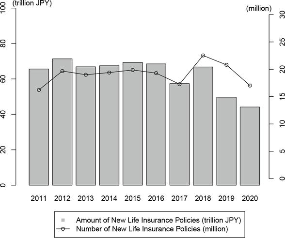
Life insurance companies play an essential role in the financial and loan markets in Japan [14]. Many of them have relied predominantly on face-to-face sales for a long period. However, since the beginning of the COVID-19 pandemic, Japanese life insurance companies were forced to temporarily suspend their face-to-face sales channels due to the nationwide declaration of a state of emergency. As shown in Figure 1, domestic sales of new policies have declined significantly since (fiscal year) 2018. According to the Life Insurance Factbook 2019 published by LIAJ, the decrease in 2019 was primarily due to lower sales of foreign currency-denominated insurance. In 2020, the conditions of domestic sales in new policies became even worse because insurance agents could not meet new customers directly. According to the monthly statistics of LIAJ, the number of new businesses reduced by 34.4$\%$ in April and 68.5$\%$ in May, on a year-on-year basis during the period of the first declaration of a state of emergency from 2020/4/7 to 2020/5/25. Moreover, even though Japanese life insurance companies resumed face-to-face sales after the state of emergency was lifted, the year-on-year decline in 2020 continued until August (14.3%).

Figure 1.

Trends in individual life insurance business (source: Life Insurance Association of Japan (LIAJ)).

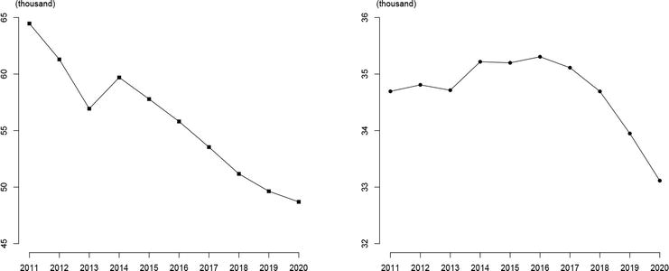
Japanese life insurance companies have changed their distribution channels over the past 10 years. It can be seen from Figure 2 that the numbers of individual and corporate agencies have been decreasing gradually in recent years. This trend should not be taken as proof that the scale of the life insurance industry has shrunk. In fact, Japanese life insurance companies have become more diversified in their sales channels due to diversifying insurance products and consumer needs and a recently increasing presence of non-traditional sales channels, such as Internet sales. Considering that life insurance companies must refrain from face-to-face sales to prevent the spread of COVID-19, a significant diversion of sales channels may lead to better performance, such as shifting from the traditional business model of face-to-face sales to online sales channels. However, sales representatives in agencies remained the primary sales channel of life insurance in 2020 [15].

Figure 2.

Distribution channels (source: Life Insurance Association of Japan (LIAJ)).

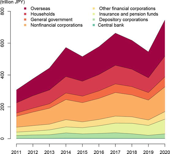
Japanese life insurance companies also play a critical role as stable institutional investors in the capital market as they hold a certain level of listed shares for a long period. Figure 3 shows the breakdown of listed shares by type of shareholder. It can be seen that the amount of listed shares held by insurance companies (insurance and pension funds) has been increasing over the past 10 years. Thus, measuring the behavior of insurance companies makes economic sense. In addition, it has been widely recognized that the current solvency margin ratio regulation introduced in 1996 does not adequately assess the valuation of liabilities and the amount of risk. This issue is expected to be solved by introducing economic value-based solvency regulations. According to the report on the economic value-based solvency framework released by the Financial Services Agency (FSA) of Japan in June 2020, the economic value-based solvency regulation will be enforced from April 2025. Since new regulations may change the business environment of Japanese life insurance companies and affect their behavior, it makes practical sense to study the past and present productive performance of Japanese life insurance companies to better prepare for the arrival of new regulations.

Figure 3.

Breakdown of listed shares by type of shareholder (source: Bank of Japan).

4.1 Inputs and outputs

To characterize the inputs and outputs of Japanese life insurance companies, we applied a value-added approach that has been commonly used in previous studies (see, e.g., [16] for a detailed discussion of the value-added approach). We considered three inputs and two outputs. The inputs were “office workers ($x_1$),” “total shareholders’ equity ($x_2$),” and “operating expenses ($x_3$).” The first two variables, office workers and total shareholders’ equity, were proxy variables for labor and capital, respectively. The operating expenses included various cost items required to operate the life insurance business, such as the selling cost, management/maintenance-related cost, and others. In contrast, the outputs were “ordinary income ($y_1$)” and “total payment of insurance benefits ($y_2$).” Ordinary predominately derives from the insurance business, such as premium income and investment-related business, the latter of which includes interest and dividend income. To account for the risk-pooling and risk-bearing capabilities of Japanese life insurance companies, we also considered the total payment of insurance benefits as a proxy output variable.

The descriptive statistics of inputs and outputs are summarized in Table 1.

Years	Statisticsa	$x_1$	$x_2$	$x_3$	$y_1$	$y_2$
2020
	mean	2780.76	3036.88	1118.93	7350.61	11960.23
	st. dev.	4148.45	4580.88	1371.91	11467.07	15925.40
	min	58.00	7.48	18.41	25.09	86.06
	max	21117.00	18952.08	5752.23	58660.91	67862.10
2019
	mean	2727.00	2799.84	1147.76	7206.73	11418.84
	st. dev.	3952.85	4297.92	1429.95	11701.79	16192.90
	min	31.00	12.68	9.66	21.10	61.08
	max	19425.00	17544.31	5987.46	61913.69	72114.03
2018
	mean	2708.49	2873.19	1190.10	7021.15	11835.05
	st. dev.	3950.21	4343.64	1463.74	12403.06	17165.93
	min	31.00	17.49	9.59	17.43	50.25
	max	19392.00	17851.78	6119.73	68688.93	79166.54
2017
	mean	2659.93	2754.62	1158.89	7059.29	11528.79
	st. dev.	3969.84	4287.69	1478.26	12414.73	16958.81
	min	34.00	9.21	9.88	13.18	42.84
	max	19515.00	18012.51	6005.71	68900.20	79529.49
2016
	mean	2643.37	2605.89	1152.84	7076.60	11649.00
	st. dev.	4000.73	4174.32	1486.14	13265.85	18130.89
	min	33.00	10.69	9.29	12.90	36.72
	max	19747.00	17412.86	5721.59	75503.23	86594.42

Table 1.

Descriptive statistics of inputs and outputs.

^a

Units of x₂, x₃, y₁, y₂: trillion yen; the unit of x₁: person.

4.2 Deterministic scenarios

In previous studies, the geometric distance function (GDF) was measured a posteriori after the projection points were computed due to its nonlinearity [2, 17]. In Section 2, we showed that for a certain deterministic scenario (see, Proposition 1.1), the value of generalized multiplicative directional distance function $M\left(\mathit{x},\mathit{y};-{\mathit{g}}^{-},{\mathit{g}}^{+}\right)$ is equal to the reciprocal of GDF. In this section, we calculated the GDP for each Japanese insurance company using the function $M\left(\mathit{x},\mathit{y};-{\mathit{g}}^{-},{\mathit{g}}^{+}\right)$.

For any $\left(\frac{\mathbf{1}}{{\mathit{\delta }}_x},{\mathit{\delta }}_y\right)\ge \left({\mathbf{1}}_m,{\mathbf{1}}_s\right)$, the function $M\left(\mathit{x},\mathit{y};-{\mathit{g}}^{-},{\mathit{g}}^{+}\right)$ can be measured by the following nonlinear programming (NLP) problem:

$$\begin{array}{l}max{\left(\prod _{i=1}^m\frac{1}{{\delta }_{x_i}}\right)}^{\frac{1}{m}}{\left(\prod _{r=1}^s{\delta }_{y_r}\right)}^{\frac{1}{s}}\\ \mathrm{s}.\mathrm{t}.\prod _{j=1}^n{x}_{\mathit{ij}}^{{\lambda }_j}\le {\left(\frac{1}{{\delta }_{x_i}}\right)}^{-g_i^{-}}{x}_{\mathit{io}},i=1,\dots ,m\\ \prod _{j=1}^n{y}_{\mathit{rj}}^{{\lambda }_j}\ge {\delta }_{y_r}^{g_r^{+}}{y}_{\mathit{ro}},r=1,\dots ,s\\ \sum _{j=1}^n{\lambda }_j=1\\ 0<{\delta }_{x_i}\le 1,{\delta }_{y_r}\ge 1,{\lambda }_j\ge 0,\forall i,r,j.\end{array}$$

Because of P3, the above problem can be equivalently reformulated as

$$\begin{array}{l}max\frac{1}{s}\sum _{j=1}^{n}log{\delta }_{y_r}-\frac{1}{m}\sum _{j=1}^{n}log{\delta }_{x_i}\\ \mathrm{s}.\mathrm{t}.\sum _{j=1}^n{\lambda }_{j}log{x}_{\mathit{ij}}\le log{x}_{\mathit{io}}+g_i^{-}log{\delta }_{x_i},i=1,\dots ,m\\ \sum _{j=1}^n{\lambda }_{j}log{y}_{\mathit{rj}}\ge log{y}_{\mathit{ro}}+g_r^{+}log{\delta }_{y_r},r=1,\dots ,s\\ \sum _{j=1}^n{\lambda }_j=1\\ log{\delta }_{x_i}\le 0,log{\delta }_{y_r}\ge 0,{\lambda }_j\ge 0,\forall i,r,j.\end{array}$$

Let $\left({\delta }_{x_i}^{\ast },{\delta }_{y_r}^{\ast },{\lambda }_j^{\ast }\right),\forall i,r,j$ be an optimal solution to the above model. Then, the GDF can be computed by

$${\varphi }^{\ast }={\left(\prod _{i=1}^m{\delta }_{x_i}^{\ast }\right)}^{\frac{1}{m}}{\left(\prod _{r=1}^s\frac{1}{{\delta }_{y_r}^{\ast }}\right)}^{\frac{1}{s}}.$$

From a theoretical perspective, an exogenously given direction vector $\left({\mathit{g}}^{-},{\mathit{g}}^{+}\right)$ is preferred for the determination of projection points. However, from a computational perspective, the direction vector in the above model can be chosen arbitrarily. In practice, the decision-makers may choose proper direction vectors depending on their purpose of performance benchmarking, or alternatively, use the direction vectors that lead to unit-invariant efficiency measures (See, e.g., [1] for detailed discussion on selecting direction vectors). In this study, we adopted $\left(g_i^{-},g_r^{+}\right)=\left(log{x}_{\mathit{io}}-{min}_{j\in \left\{1,\dots ,n\right\}}log{x}_{\mathit{ij}},{max}_{j\in \left\{1,\dots ,j\right\}}log{y}_{\mathit{rj}}-log{y}_{\mathit{ro}}\right),\forall i,r$ to derive the unit-invariant GDF efficiencies.

The estimated GDF efficiencies are reported in Table 2. There were three efficient companies over the fiscal years 2016–2020: DMU05 (AEON Allianz Life Insurance Co., Ltd.), DMU18 (The Dai-ichi Frontier Life Insurance Co., Ltd.), and DMU41 (Rakuten Life Insurance Co., Ltd.). These companies can be seen as adopting best practices that were sustainable given the challenges of a changing business environment over the whole period. In addition, we also found that the Japanese life insurance industry is experiencing a downturn in performance, as the average efficiency score declined from 2016 to 2020.

DMUsa	2020	2019	2018	2017	2016
DMU01	0.501	0.486	0.6	0.61	0.677
DMU02	1	1	1	0.3	0.3
DMU03	0.433	0.449	0.557	0.538	0.588
DMU04	0.437	0.44	0.504	0.519	0.557
DMU05	1	1	1	1	1
DMU06	0.438	0.418	0.342	0.471	0.759
DMU07	0.638	0.619	0.966	1	0.451
DMU08	0.618	0.555	0.692	0.815	0.876
DMU09	0.475	0.45	0.57	0.616	0.705
DMU10	0.486	0.551	0.448	0.621	0.628
DMU11	1	0.779	0.38	1	1
DMU12	0.512	0.516	0.652	0.628	0.673
DMU13	0.467	0.446	0.52	0.504	0.548
DMU14	0.5	0.496	0.584	0.567	0.6
DMU15	0.591	1	0.621	0.828	1
DMU16	0.453	0.456	0.582	0.574	0.602
DMU17	0.594	0.531	0.659	0.635	0.728
DMU18	1	1	1	1	1
DMU19	0.472	0.485	0.604	0.599	0.637
DMU20	0.468	0.482	0.598	0.57	0.618
DMU21	0.492	0.501	0.656	0.61	0.684
DMU22	1	1	1	0.6	0.613
DMU23	0.736	0.672	0.616	0.767	1
DMU24	0.493	0.506	0.66	0.674	0.749
DMU25	0.662	0.668	0.74	0.343	0.344
DMU26	0.336	0.343	0.343	0.382	0.303
DMU27	0.587	1	0.544	0.589	0.641
DMU28	0.462	0.479	0.604	0.624	0.661
DMU29	0.811	0.709	0.601	0.696	0.759
DMU30	0.554	0.558	0.722	0.777	0.87
DMU31	0.59	0.588	0.738	0.786	0.821
DMU32	0.695	0.605	1	1	1
DMU33	0.447	0.46	0.566	0.543	0.584
DMU34	1	0.708	0.907	1	0.926
DMU35	0.401	0.398	0.305	0.313	0.309
DMU36	0.396	0.423	0.491	0.492	0.523
DMU37	0.553	0.55	0.716	0.663	0.824
DMU38	0.413	0.45	0.346	0.419	0.4
DMU39	0.404	0.438	0.309	0.324	0.321
DMU40	0.419	0.456	0.421	0.539	0.5
DMU41	1	1	1	1	1
mean	0.598	0.602	0.638	0.647	0.678
st. dev	0.208	0.204	0.208	0.206	0.215

Table 2.

Results of GDF efficiencies.

^a

The number of DMUs follows the order of the member companies of the Life Insurance Association of Japan (LIAJ), as released on November 2, 2021. We excluded HANASAKU LIFE INSURANCE Co., Ltd. from the sample because it is a new member as of April 1, 2019.

The average values of $\left({\mathit{\delta }}_{\mathit{x}}^{\ast },\frac{\mathbf{1}}{{\mathit{\delta }}_{\mathit{y}}^{\ast }}\right)$ are summarized in Table 3. The parameters ${\mathit{\delta }}_x^{\ast }$ and $\frac{\mathbf{1}}{{\mathit{\delta }}_y^{\ast }}$ can be interpreted as the element-specific efficiencies for inputs and outputs, respectively. It can be seen from Table 3 that the input “total shareholders’ equity ($x_2$)” had the highest average efficiency score versus the other inputs and outputs over the period 2016–2020 (the mean of ${\delta }_{x_2}^{\ast }$ was 0.861). The second highest average efficiency score was achieved by “operating expenses ($x_3$)” (the mean of ${\delta }_{x_3}^{\ast }$ was 0.808). This indicates that Japanese life insurance companies have good performance in funding-related inputs. By contrast, the input “office workers ($x_1$)” had the lowest average efficiency score (the mean of ${\delta }_{x_1}^{\ast }$ was 0.67), which implies that Japanese life insurance companies have relatively poor performance in human resources. This may be due to the paradigm shift in the face of an increasing number of new sales channels. Additionally, since Japanese life insurance companies could not meet new customers directly in order to prevent the spread of COVID-19 in 2020, the decreased efficiency score in 2020 compared to 2019 may due to the impact of the nationwide declaration of a state of emergency. However, further investigations are needed regarding this issue.

Year	${\delta }_{x_1}^{\ast }$	${\delta }_{x_2}^{\ast }$	${\delta }_{x_3}^{\ast }$	$\frac{1}{{\delta }_{y_1}^{\ast }}$	$\frac{1}{{\delta }_{y_2}^{\ast }}$
2020	0.667	0.925	0.751	0.661	0.73
2019	0.704	0.867	0.85	0.65	0.699
2018	0.648	0.85	0.803	0.794	0.77
2017	0.651	0.833	0.815	0.782	0.78
2016	0.681	0.828	0.819	0.798	0.821
mean	0.67	0.861	0.808	0.737	0.76

Table 3.

Results of the estimated $\left({\mathit{\delta }}_{\mathit{x}}^{\ast },{\frac{\mathbf{1}}{{\mathit{\delta }}_{\mathit{y}}}}^{\ast }\right)$.

4.3 Stochastic scenarios

Compared with the generalized multiplicative directional distance function $M\left(\mathit{x},\mathit{y};-{\mathit{g}}^{-},{\mathit{g}}^{+}\right)$, the proposed stochastic multiplicative directional distance function (SMDDF) $\tilde{M}\left(\mathit{x},\mathit{y};-{\mathit{g}}^{-},{\mathit{g}}^{+}\right)$ is capable of capturing the statistical variation present in the observed data. To facilitate comparison, we applied the same direction vector used in Section 4.2 to estimate the SMDDF. The estimated coefficients characterizing the tangent hyperplanes of the concave SMDDF for all DMUs are summarized in Table 4.

Years	Statisticsa	${\upsilon }^{\ast }$	${\zeta }_1^{\ast }$	${\zeta }_2^{\ast }$	${\zeta }_3^{\ast }$	${\gamma }_1^{\ast }$	${\gamma }_2^{\ast }$
2020
	mean	−595.781	719.704	324.489	858.349	424.36	24.15
	st. dev.	23506.536	4604.907	2075.796	3837.448	2714.835	118.149
	min	−56133.412	0.001	0.015	0	0.001	0
	max	121722.234	29486.327	13291.882	17161.857	17383.801	591.261
	$†$DMU02	−38155.613	2.357	13291.882	1.082	0.139	0.14
	$†$DMU05	−56133.412	7.441	0.453	17161.857	0.193	0.193
	$†$DMU11	−51901.156	29486.327	0.44	1.423	0.19	0.202
	$†$DMU41	121722.234	0.455	0.166	0.286	17383.801	591.261
2019
	mean	−191.393	461.661	792.405	200.862	232.605	378.179
	st. dev.	25869.435	2954.279	4945.889	851.021	1486.929	1850.085
	min	−95754.967	0.002	0	0	0.002	0
	max	126825.46	18916.892	30887.494	3610.85	9521.375	9064.062
	$†$DMU02	−95754.967	1.197	30887.494	0.618	0.125	0.126
	$†$DMU05	−38947.375	18916.892	0.652	3610.85	0.221	0.22
	$†$DMU41	126825.46	0.393	0.187	0.241	9521.375	9064.062
2018
	mean	−1174.219	221.483	822.733	286.871	165.586	173.732
	st. dev.	20711.798	1416.317	5001.333	1281.837	1058.141	932.863
	min	−98572.938	0.002	0	0	0.005	0
	max	81008.126	9069.146	30422.438	5732.792	6775.741	5024.123
	$†$DMU02	−98572.938	1.303	30422.438	0.712	0.122	0.119
	$†$DMU05	−30606.077	9069.146	3.194	5732.792	0.222	0.226
	$†$DMU41	81008.126	0.419	0.2	0.25	6775.741	5024.123
2017
	mean	2470.9	117.05	286.855	338.048	397.955	277.471
	st. dev.	27075.687	747.405	1742.883	1547.98	2545.768	1412.526
	min	−59913.335	0.004	0	0	0.004	0
	max	161196.848	4786.051	10601.869	7093.989	16301.242	7202.949
	$†$DMU05	−59913.335	4786.051	10601.869	7093.989	0.262	0.267
	$†$DMU41	161196.848	0.394	0.172	0.232	16301.242	7202.949
2016
	mean	1543.176	350.93	112.891	35.068	299.912	113.54
	st. dev.	15406.705	1717.644	694.418	222.124	1641.759	714.694
	min	−29985.44	0	0	0.01	0	0
	max	93237.186	8415.021	4280.92	1422.665	8992.456	4520.656
	$†$DMU05	−29985.44	8415.021	4280.92	1422.665	0.269	0.279
	$†$DMU41	93237.186	0.414	0.192	0.244	8992.456	4520.656

Table 4.

Descriptive statistics of the estimated coefficients.

^a

† represents the DMU with extremely large or extremely small coefficients.

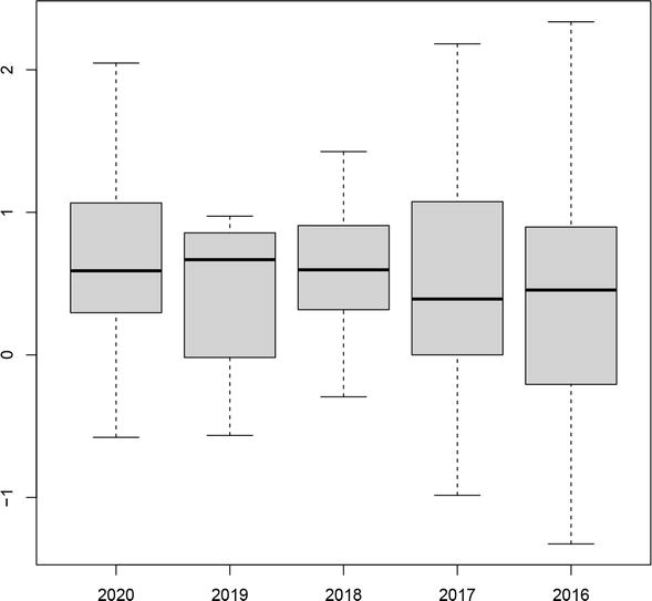
From Table 4, it is clear that the estimated coefficients exhibited significant variance over the period 2016–2020. However, few DMUs had extremely large or extremely small coefficients, and the estimated coefficients of most of the observed DMUs were in the range 0 to 1. This can be intuitively understood, for example, from the box plot of the intercepts ${\upsilon }^{\ast }$ excluding the extreme values, as shown in Figure 4. We also report the DMUs with extreme values of estimated coefficients for each year in Table 4. Since the coefficients characterize the tangent hyperplane of the concave SMDDF of each DMU, DMUs with extreme values of the estimated coefficients may affect the shape of the estimated concave SMDDF and be identified as efficient DMUs. Indeed, all DMUs with extreme estimated coefficients are also evaluated as efficient DMUs in the deterministic scenario, as shown in Table 2. Moreover, we found that DMU02 is efficient in the deterministic scenario for the period 2018–2020. This observation is consistent with the results of the stochastic scenario. From Table 4, the period when DMU02 had extreme values of the estimated coefficients was also 2018–2020. However, the same is not true for DMU11. DMU11 was efficient in the deterministic scenario in 2016, 2017, and 2020, whereas its estimated coefficients were extreme only in 2020. However, this does not mean that DMU11 is not efficient, because technically, we cannot exclude the possibility that DMUs without extreme estimated coefficients cannot affect the shape of the estimated concave SMDDF. Regarding the efficient DMUs without extreme estimated coefficients in Table 2, they may be overestimated because the deterministic model ignored the impact of random errors.

Figure 4.

Box plot of the intercepts ${\upsilon }^{\ast }$.

The results of the deterministic scenario show that the Japanese life insurance industry exhibited worse performance between 2016 and 2020. By contrast, the results of the stochastic scenario in Table 5 show that the estimated average inefficiency ${\mu }^{\ast }$ increased from 2016 to 2019 and then decreased, which implies that the Japanese life insurance industry likely performed better in 2020 than in 2019. Since the efficiency scores in 2020 exhibited slightly more variation than those in 2019, as shown in Table 2, the difference in the average performance between the deterministic and stochastic scenarios may be due to the impact of random error. Nevertheless, considering that both approaches have a small range of variation in the average (in)efficiencies (i.e., the deterministic scenario: $\left[\mathrm{0.004,0.08}\right]$; the stochastic scenario: $\left[\mathrm{0.009,0.056}\right]$), we conclude that the Japanese insurance industry exhibited relatively stable performance during 2016–2020.

	2020	2019	2018	2017	2016
${\mu }^{\ast }$	0.144	0.166	0.15	0.119	0.11

Table 5.

Results of the estimated expected value of the logarithm of inefficiencies ${\mu }^{\ast }$.

5. Conclusions

This study considers a flexible structure of production technology that is constructed based on geometric convexity assumption. We investigated the relationship between the generalized multiplicative directional distance function (GMDDF) and geometric distance function (GDF) based on a given geometric convex production possibility set. We show that, given a deterministic scenario, the multiplication of GMDDF and GDF for the observed DMUs has the same value as the GMDDF calculated for the projection points. Based on this relationship, the GDF efficiencies can be easily measured by a DEA methodology. We also proposed a stochastic multiplicative directional distance function (SMDDF) in which all inputs and outputs are considered random variables. Given a stochastic scenario, we show that the SMDDF can be formulated as a CNLS problem. The productive performance of Japanese life insurance companies was investigated. Several companies were identified as efficient DMUs from both the results of the deterministic and stochastic scenarios. These companies can be used as projections for improving inefficiencies. Moreover, it seems that Japanese life insurance companies have a good performance in funding-related inputs since “total shareholders’ equity” and “operating expenses” were more efficient than were other inputs and outputs. By contrast, many of the Japanese life insurance companies may have suffered from poor performance in human resources. Furthermore, both the deterministic and stochastic scenarios suggest a decline in the average performance of the whole life insurance industry during 2016-2019. However, since the variations of average (in)efficiencies over the years are small, it is reasonable to conclude that the Japanese life insurance industry achieved relatively stable performance in the previous five years.

Abbreviations

CNLS	convex nonparametric least squares
DEA	data envelopment analysis
DMU	decision-making unit
FSA	financial services agency
GDF	geometric distance function
GMDDF	generalized multiplicative directional distance function
LIAJ	Life Insurance Association of Japan
NLP	nonlinear programming
QP	quadratic programming
SMDDF	stochastic multiplicative directional distance function
StoNED	stochastic nonparametric envelopment of data

References

1.Mehdiloozad M, Sahoo BK, Roshdi I. A generalized multiplicative directional distance function for efficiency measurement in DEA. European Journal of Operational Research. 2014;232(3):679-688
2.Portela MCAS, Thanassoulis E. Profitability of a sample of Portuguese bank branches and its decomposition into technical and allocative components. European Journal of Operational Research. 2005;162(3):850-866
3.Charnes A, Cooper WW, Rhodes E. Measuring the efficiency of decision making units. European Journal of Operational Research. 1978;2(6):429-444
4.Banker RD, Maindiratta A. Piecewise loglinear estimation of efficient production surfaces. Management Science. 1986;32(1):126-135
5.Aigner D, Lovell CK, Schmidt P. Formulation and estimation of stochastic frontier production function models. Journal of Econometrics. 1977;6(1):21-37
6.Kuosmanen T. Representation theorem for convex nonparametric least squares. The Econometrics Journal. 2008;11(2):308-325
7.Banker RD, Charnes A, Cooper WW. Some models for estimating technical and scale inefficiencies in data envelopment analysis. Management Science. 1984;30(9):1078-1092
8.Färe R, Grosskopf S, Lovell CK. The Measurement of efficiency of production. Vol. 6. Dordrecht: Springer Science & Business Media; 1985
9.Majumdar M, Roy S. Non-convexity, discounting and infinite horizon optimization. Journal of Nonlinear and Convex Analysis. 2009;10:1-18
10.Valadkhani A, Roshdi I, Smyth R. A multiplicative environmental DEA approach to measure efficiency changes in the world’s major polluters. Energy Economics. 2016;54:363-375
11.Roshdi I, Hasannasab M, Margaritis D, Rouse P. Generalised weak disposability and efficiency measurement in environmental technologies. European Journal of Operational Research. 2018;266(3):1000-1012
12.Afriat SN. Efficiency estimation of production functions. International Economic Review. 1972;13(3):568-598
13.Kuosmanen T, Johnson A. Modeling joint production of multiple outputs in StoNED: Directional distance function approach. European Journal of Operational Research. 2017;262(2):792-801
14.Fukuyama H. Investigating productive efficiency and productivity changes of Japanese life insurance companies. Pacific-Basin Finance Journal. 1997;5(4):481-509
15.Nobuyasu U. Japan’s insurance market 2021. Tokyo: The Toa Reinsurance Company, Limited; 2021
16.Eling M, Luhnen M. Frontier efficiency methodologies to measure performance in the insurance industry: Overview, systematization, and recent developments. The Geneva Papers on Risk and Insurance-Issues and Practice. 2010;35(2):217-265
17.Portela MCAS, Thanassoulis E. Malmquist indexes using a geometric distance function (GDF). Application to a sample of Portuguese bank branches. Journal of Productivity Analysis. 2006;25(1):25-41
Written By
Yu Zhao
Submitted: 02 March 2022Reviewed: 03 March 2022Published: 24 June 2022
Open access peer-reviewed chapter