Perspective Chapter: On the Morse Property for the Distance Function of a Robot Arm

Abstract

Morse theory plays a central role when we study the configuration space of various mechanical linkages. As an important linkage, we consider the planar robot arm. It is known that the distance function on its configuration space is a Morse function. On the other hand, for a fixed angle $\theta$, we consider the spatial robot arm whose adjacent bond angles are $\theta$. In chemistry, such an arm is used as a model for protein backbones and has been studied extensively. We consider the distance function on its configuration space. The purpose of this chapter is threefold: First, we study whether the distance function is a Morse function. Second, we determine the minimum and maximum values of the function. Consider the case that the arm consists of four bars. Then our third purpose is to study how the distance function is different from the usual Morse function on the torus.

1. Introduction

1.1 Mathematical study of robotics

A motion planning problem studies a sequence of valid configurations of a given mechanical linkage. The problem is interesting because it has many important robotics applications. Some impressive results are obtained in Refs. [1, 2, 3]. Mathematicians are also interested in the configuration space of mechanical linkages. Here, the configuration space is defined as the space of all possible shapes of the linkage. Robot arms are quite important examples of mechanical linkages: in molecular biology, the arms describe molecular shapes and the arms play a central role in statistical shape theory.

Morse theory plays a central role when we study the configuration space of robot arms. (See Ref. [4] for the excellent survey with emphasis on the Morse theory.) In differential topology, Morse theory is a powerful tool to analyze spaces. A function $f:M\to \mathbb{R}$ on a manifold $M$ is called a Morse function if every critical point of $f$ is nondegenerate. Morse functions play a principal role in the Morse theory.

The Morse property for the distance function on the configuration space of the robot arm in ${\mathbb{R}}^2$ is studied well. The purpose of this chapter is to consider the distance function on the configuration space of another robot arm.

1.2 The most famous mechanical linkage: The robot arm in ${\mathbb{R}}^2$

We consider the robot arm in ${\mathbb{R}}^2$, which consists of $n$ bars of length $\left(1,1,\dots ,1\right)$ connected by revolving joints. The initial point of the robot arm is fixed at $O$. The configuration space of the robot arm is

$$W_n=\left\{\left(u_1,\dots ,u_n\right)\in {\left(S^1\right)}^n\right\}/\mathit{SO}\left(2\right).$$E1

By the $\mathit{SO}\left(2\right)$-action, we may normalize $u_1$ uniquely to be $\left(1,0\right)$. Hence, there is an identification

$$W_n=\left\{\left(u_1,\dots ,u_n\right)\in {\left(S^1\right)}^n|u_1=(1,0)\right\}.$$E2

From (2), we have

$$W_n={\left(S^1\right)}^{n-1}.$$E3

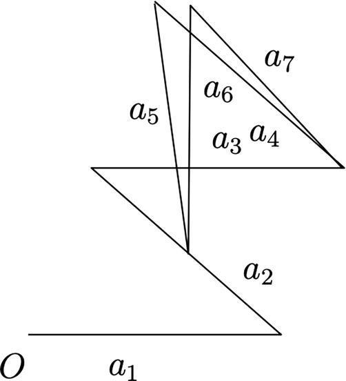
Hereafter, we will use (2) as the definition of $W_n$. (See the following Figure 1.)

Figure 1.

An element of $W_4$.

1.3 The distance function on $W_n$: Remarkable results

We define the function

$${\mu }_n:W_n\to \mathbb{R}$$E4

by

$${\mu }_n\left(u_1,\dots ,u_n\right)={‖\sum _{i=1}^n{u}_i‖}^2.$$E5

Note that ${\mu }_n^{-1}\left(0\right)$ is the equilateral polygon space, which is a critical manifold of dimension $n-3$. In order to avoid critical manifolds of positive dimension, we consider the following restriction of ${\mu }_n$:

$${\left.{\mu }_n\right|}_{W_n\backslash {\mu }_n^{-1}\left(0\right)}:W_n\backslash {\mu }_n^{-1}\left(0\right)\to \mathbb{R}.$$E6

It is proved in Refs. [5, 6] (see also [[4], Lemma 1.4]) that (6) is a Morse function. More precisely, a critical point corresponds to the case that $u_i=\pm u_1$ for $2\le i\le n$. Moreover, the index of a critical point is determined explicitly. This Morse property has many interesting applications. Among them, the following two applications are particularly important:

• It is proved in Ref. [7] that polygon spaces are obtained from the sphere by successive surgeries.

• The homology groups of planar polygon spaces are determined in Ref. [8].

1.4 A new robot arm: A mathematical model for protein backbones

We fix $\theta \in \left(0,\pi \right)$. The robot arm in ${\mathbb{R}}^3$ with all bond angles $\theta$, permitting “dihedral” spinning about each edge, has been used to model the geometry of protein backbones [9, 10]. Let $X_n\left(\theta \right)$ be the configuration space of the arm. That is, $X_n\left(\theta \right)$ is defined as the space of all possible shapes of our arm. (See Section 2 for more details.)

1.5 The main problem

Let $f_{n,\theta }:X_n\left(\theta \right)\to \mathbb{R}$ be the distance function. In this chapter, we study three problems concerning $f_{n,\theta }$. (See Problem 2.7.) The most important problem is given as follows: Does $f_{n,\theta }$ satisfy the Morse property?

1.6 Motivation for the main problem

We explain the motivation for the above main problem. Recall that we have $W_n={\left(S^1\right)}^{n-1}$. Similarly, we can prove that $X_n\left(\theta \right)={\left(S^1\right)}^{n-2}$. Moreover, ${\mu }_n$ and $f_{n,\theta }$ are defined to be the distance functions. Now since ${\mu }_n$ satisfies the Morse property, it is natural to ask whether $f_{n,\theta }$ also satisfies the property.

1.7 Previous study on $f_{n,\theta }$

Although some chemists are interested in a special element of $X_n\left(\theta \right)$, nobody has studied the space $X_n\left(\theta \right)$ nor the function $f_{n,\theta }$. Hence, our results are completely new.

1.8 Summary of the main result

The function $f_{n,\theta }$ satisfies the Morse property if and only if $n=3$ or $5$.

1.9 Organization of this chapter

In Section 2, we first prepare notations. Then we pose three problems in Problem 2.7. Finally, we summarize the known results in Theorems 2.9, 2.10 and 2.11. In Section 3, we state our main theorems. Theorems A and B are answers to the first problem of Problem 2.7. Theorems C and D are answers to the second problem. Theorem E is an answer to the third problem. In Section 4, we construct submanifolds of $X_n\left(\theta \right)$, which are used in Section 5. In Section 5, we prove our main theorems. In Section 6, we state the conclusions.

2. Preliminaries

We define the space $X_n\left(\theta \right)$ as follows: We fix $\theta \in \left(0,\pi \right)$ and define the following space:

$$A_n\left(\theta \right)≔\left\{\left(a_1,\dots ,a_n\right)\in {\left(S^2\right)}^n|⟨a_i,a_{i+1}⟩=-cos\theta \left(1\le i\le n-1\right)\right\},$$E7

where $⟨,⟩$ denotes the standard inner product on ${\mathbb{R}}^3$. Let $\mathit{SO}\left(3\right)$ act on $A_n\left(\theta \right)$ diagonally. Then we set

$$X_n\left(\theta \right)≔A_n\left(\theta \right)/\mathit{SO}\left(3\right).$$E8

Using the $\mathit{SO}\left(3\right)$-action, we can normalize $a_1$ and $a_2$ to be

$$a_1=\left(\mathrm{1,0,0}\right)\text{and}{a}_2=\left(-cos\theta ,sin\theta ,0\right).$$E9

Then similarly to (2), we use the following identification:

$$X_n\left(\theta \right)=\left\{\left(a_1,\dots ,a_n\right)\in A_n\left(\theta \right)|a_1\text{and}{a}_2\mathrm{are}\mathrm{as}\text{in}\left(9\right)\right\}.$$E10

Hereafter, we use (10) as the definition of $X_n\left(\theta \right)$. (See the following Figure 2.)

Figure 2.

An element of $X_4\left(\theta \right)$.

Lemma 2.1. There is a diffeomorphism

$$T:{\left(S^1\right)}^{n-2}\to X_n\left(\theta \right).$$E11

Proof: We prove in the same way as given in [[11], Lemma 13] and [[12], Lemma 7]. From an element

$$\left(e^{i{\varphi }_1},\cdots ,e^{i{\varphi }_{n-2}}\right)\in {\left(S^1\right)}^{n-2},$$E12

we construct the element $\left(a_1,\cdots ,a_n\right)\in X_n\left(\theta \right)$ as follows: In the process of constructing $a_i$, we also construct the elements $n_i\in S^2$ such that $⟨a_i,n_i⟩=0$. We set

$$a_{i+2}≔-\left(cos\theta \right)a_{i+1}+\left(sin\theta cos{\varphi }_i\right)n_{i+1}+\left(sin\theta sin{\varphi }_i\right)a_{i+1}\times n_{i+1}$$E13

and

$$n_{i+2}≔-\left(sin\theta \right)a_{i+1}-\left(cos\theta cos{\varphi }_i\right)n_{i+1}-\left(cos\theta sin{\varphi }_i\right)a_{i+1}\times n_{i+1},$$E14

where $a_{i+1}\times n_{i+1}$ denotes the cross product.

We set

$$\begin{array}{l}{a}_1=\left(\mathrm{1,0,0}\right),n_1=\left(\mathrm{0,1,0}\right)\\ a_2=\left(-cos\theta ,sin\theta ,0\right)\text{and}{n}_2=\left(-sin\theta ,-cos\theta ,0\right).\end{array}$$E15

From (13) and (14) for $i=1$, we obtain $a_3$ and $n_3$. Next from (13) and (14) for $i=2$, we obtain $a_4$ and $n_4$. Repeating this process, we obtain $a_i$ and $n_i$ for $1\le i\le n$. Now we define $T$ by

$$T\left(e^{i{\varphi }_1},\cdots ,e^{i{\varphi }_{n-2}}\right)=\left(a_1,\cdots ,a_n\right).$$E16

From the construction, $T$ is a diffeomorphism.

Notation 2.2. We define the element $\left[{\varphi }_1,\dots ,{\varphi }_{n-2}\right]\in X_n\left(\theta \right)$ by

$$\left[{\varphi }_1,\dots ,{\varphi }_{n-2}\right]≔T\left(e^{i{\varphi }_1},\cdots ,e^{i{\varphi }_{n-2}}\right),$$E17

where the diffeomorphism $T$ is constructed in Lemma 2.1.

Lemma 2.3. Assume that ${\varphi }_i\in \left\{0,\pi \right\}$ for $1\le i\le n-2$. We write $\left[{\varphi }_1,\dots ,{\varphi }_{n-2}\right]=\left(a_1,\dots ,a_n\right)$. Then the following results hold:

1. For $1\le i\le n-2$, $a_i$ is a vector in ${\mathbb{R}}^2$.

2. If ${\varphi }_j=\pi$, then we have $a_{j+2}=a_j$. (See the left of the following Figure 3.) On the other hand, if ${\varphi }_j=0$, then $a_{j+2}$ is as given in the right of the following Figure 3.

Figure 3.

Left: ${\varphi }_j=\pi$. Right: ${\varphi }_j=0$.

Proof of Lemma 2.3: The lemma is clear from the construction of the diffeomorphism $T$ in Lemma 2.1.

Using Lemma 2.3, we give the following:

Definition 2.4.

1. Consider the point $\left[{\varphi }_1,\dots ,{\varphi }_{n-2}\right]$ such that ${\varphi }_i=\pi$ for $1\le i\le n-2$. We denote the unique point by $P_{n,\theta }$. (See the following Figure 4.)

2. Consider the point $\left[{\varphi }_1,\dots ,{\varphi }_{n-2}\right]$ such that ${\varphi }_i=0$ for $1\le i\le n-2$. We denote the unique point by $Q_{n,\theta }$. (See the following Figure 5.)

Figure 4.

$P_{4,\theta }$.

Figure 5.

$Q_{4,\theta }$.

Definition 2.5.

1. We define the function

   $$f_{n,\theta }:X_n\left(\theta \right)\to \mathbb{R}$$E18

   by

   $$f_{n,\theta }\left(a_1,\dots ,a_n\right)={‖\sum _{i=1}^n{a}_i‖}^2.$$E19

2. We also define the function

   $$d_{n,\theta }:X_n\left(\theta \right)\to \mathbb{R}$$E20

   by

   $$d_{n,\theta }≔\sqrt{f_{n,\theta }}.$$E21

3. We also set

$${\mathrm{\ell }}_{n,\theta }≔min{d}_{n,\theta }\left(X_n\left(\theta \right)\right)\text{and}{L}_{n,\theta }≔max{d}_{n,\theta }\left(X_n\left(\theta \right)\right).$$E22

Remark 2.6. The point $P_{n,\theta }$ in Definition 2.4 (i) is particularly important. In fact, as we see in Proposition 4.1, $P_{n,\theta }$ is a degenerate critical point of $f_{n,\theta }$ when $n$ is even.

The purpose of this chapter is to study the three items in the following:

Problem 2.7. (i) We study whether $f_{n,\theta }$ satisfies the same Morse property as ${\mu }_n$.

(ii) We obtain explicit formulae for $L_{n,\theta }$ and ${\mathrm{\ell }}_{n,\theta }$.

(iii) We study how the level set $d_{4,\theta }^{-1}\left(r\right)$ changes as $r$ moves in $\mathbb{R}$.

Background 2.8. We explain the background for the items in Problem 2.7.

(i) The motivation for Problem 2.7 (i) is explained in Subsection 1.6. More precisely, recall that ${\mu }_n$ in (4) is a function on ${\left(S^1\right)}^{n-1}$. On the other hand, by Lemma 2.1, we can regard $f_{n,\theta }$ as a function on ${\left(S^1\right)}^{n-2}$. Then it is natural to ask whether $f_{n,\theta }$ has the same Morse property as ${\mu }_n$.

(ii) About Problem 2.7 (ii), it is known that a point of $X_n\left(\theta \right)$ attains $L_{n,\theta }$ or ${\mathrm{\ell }}_{n,\theta }$. (See Theorem 2.10.) Hence, our task is to obtain explicit formulae for $L_{n,\theta }$ and ${\mathrm{\ell }}_{n,\theta }$.

(iii) About Problem 2.7 (iii), as we stated in Remark 2.6, $P_{4,\theta }$ is a degenerate critical point of $f_{4,\theta }$. Hence, we cannot apply the Morse theory for $f_{4,\theta }$. Instead, we determine the level set $d_{4,\theta }^{-1}\left(r\right)$ for each $r\in \mathbb{R}$. In particular, we see from our result that $f_{4,\theta }$ is in fact different from the usual Morse function on ${\left(S^1\right)}^2$.

We summarize the known results in the following Theorems 2.9, 2.10 and 2.11. First, it is clear that ${\mu }_n^{-1}\left(0\right)$ is always nonempty. On the other hand, we have the following:

Theorem 2.9 [13].

1. When $n$ is odd, we have

   $$f_{n,\theta }^{-1}\left(0\right)=\left\{\begin{array}{ll}\varnothing ,& \mathit{\text{if}}0<\theta <\frac{\pi }{n}\mathit{\text{or}}\frac{n-2}{n}\pi <\theta <\pi ,\\ \left\{\mathit{one}\mathit{\text{point}}\right\},& \mathit{\text{if}}\theta =\frac{\pi }{n}\mathit{\text{or}}\frac{n-2}{n}\pi ,\\ a\mathit{\text{space of dimension}}max\left\{n-5,0\right\},& \mathit{\text{if}}\frac{\pi }{n}<\theta <\frac{n-2}{n}\pi .\end{array}\right.$$E23

2. When $n$ is even, we have

   $$f_{n,\theta }^{-1}\left(0\right)=\left\{\begin{array}{ll}\varnothing ,& \mathit{\text{if}}0<\theta <\frac{n-2}{n},\\ \left\{\mathit{one}\mathit{\text{point}}\right\},& \mathit{\text{if}}\theta =\frac{n-2}{n}\pi ,\\ a\mathit{\text{space of dimension}}max\left\{n-5,0\right\},& \mathit{\text{if}}\frac{n-2}{n}\pi <\theta <\pi .\end{array}\right.$$E24

Proof: Note that $f_{n,\theta }^{-1}\left(0\right)$ is the configuration space of equilateral spatial $n$-gons whose first $\left(n-1\right)$ bond angles are $\theta$. In Ref. [13], the space is denoted by ${\mathcal{P}}_n^{n-1}\left(\theta \right)$ and the corresponding results are proved using the notation ${\mathcal{P}}_n^{n-1}\left(\theta \right)$. If we rewrite ${\mathcal{P}}_n^{n-1}\left(\theta \right)$ to $f_{n,\theta }^{-1}\left(0\right)$, then we obtain the theorem.

We state our second known result. Recall that $P_{n,\theta }$ and $Q_{n,\theta }$ are defined in Definition 2.4.

Theorem 2.10 [14, 15].

1. The number $L_{n,\theta }$ is attained uniquely by $P_{n,\theta }$.

2. If ${\mathrm{\ell }}_{n,\theta }>0$, then ${\mathrm{\ell }}_{n,\theta }$ is attained uniquely by $Q_{n,\theta }$.

Let ${\mathcal{M}}_4\left(\theta \right)$ be the configuration space of equilateral and equiangular squares. In our notation, ${\mathcal{M}}_4\left(\theta \right)$ is defined as

$${\mathcal{M}}_4\left(\theta \right)=\left\{\left(a_1,\dots ,a_4\right)\in X_4\left(\theta \right)|\sum _{i=1}^4{a}_i=\left(\mathrm{0,0,0}\right)\text{and}⟨a_4,a_1⟩=-cos\theta \right\}.$$E25

Then our third known result is the following:

Theorem 2.11 [16]. We have

$${\mathcal{M}}_4\left(\theta \right)=\left\{\begin{array}{ll}\varnothing ,& \mathit{\text{if}}\frac{\pi }{2}<\theta <\pi ,\\ \left\{\mathit{one}\mathit{\text{point}}\right\},& \mathit{\text{if}}\theta =\frac{\pi }{2},\\ \left\{\mathit{two}\mathit{\text{points}}\right\},& \mathit{\text{if}}0<\theta <\frac{\pi }{2}.\end{array}\right.$$E26

The following Figure 6 illustrates the case $\theta =\frac{\pi }{2}$. Note that when $\theta =\frac{\pi }{2}$ we have ${\mathcal{M}}_4\left(\theta \right)=Q_{4,\theta }$, where $Q_{4,\theta }$ is illustrated in Figure 5.

Figure 6.

The element of ${\mathcal{M}}_4\left(\frac{\pi }{2}\right)$.

On the other hand, the following Figure 7 illustrates the case $0<\theta <\frac{\pi }{2}$. The two figures in Figure 7 are mirror images of each other with respect to the $\mathit{xy}$-plane.

Figure 7.

The two elements of ${\mathcal{M}}_4\left(\theta \right)$ for $0<\theta <\frac{\pi }{2}$.

3. Main results

First, we give an answer to Problem 2.7 (i). (See Example 3.2, Theorems A and B.) Theorem 2.9 tells us that if $n\ge 6$, then $f_{n,\theta }^{-1}\left(0\right)$ is a critical manifold of positive dimension. In order to avoid such a manifold, we remove $f_{n,\theta }^{-1}\left(0\right)$ from the domain of $f_{n,\theta }$ in the same way as given in (1.3):

Notation 3.1. We abbreviate the following restriction by $g_{n,\theta }$:

$${\left.f_{n,\theta }\right|}_{X_n\left(\theta \right)\backslash f_{n,\theta }^{-1}\left(0\right)}:X_n\left(\theta \right)\backslash f_{n,\theta }^{-1}\left(0\right)\to \mathbb{R}.$$E27

We begin by studying the most elementary case in the following:

Example 3.2. Consider the case $n=3$. By Theorem 2.9 (i), $f_{3,\theta }^{-1}\left(0\right)$ consists of at most finite points. Hence, we may consider $f_{3,\theta }$ for $g_{3,\theta }$. We fix $\theta$ and use the diffeomorphism $T:S^1\to X_3\left(\theta \right)$ in Lemma 2.1. Then we can write $f_{3,\theta }\circ T$ as

$$\left(f_{3,\theta }\circ T\right)\left(e^{i{\varphi }_1}\right)=c_1+c_{2}cos{\varphi }_1$$E28

for some $c_1>0$ and $c_2<0$. Hence for all $\theta$, $f_{3,\theta }$ is a Morse function with two critical points.

Proof of Example 3.2: First, using (13), we compute $a_3$. Second, using (19), we compute $\left(f_{3,\theta }\circ T\right)\left(e^{i{\varphi }_1}\right)$. Then we obtain (28). Note that (28) implies that $f_{3,\theta }\circ T$ is essentially the same as the usual Morse function on $S^1$.

Next, we consider the case $n=5$. Similarly to Example 3.2, we may consider $f_{5,\theta }$ for $g_{5,\theta }$.

Theorem A.

1. We set

   $$\alpha ≔2arccot\left(\sqrt{7}\right)\approx 0.23\pi \mathit{\text{and}}\beta ≔2arctan\left(\sqrt{\frac{3+2\sqrt{5}}{11}}\right)\approx 0.43\pi .$$E29

   Using this, we set

   $$\mathrm{\Theta }≔\left(0,\pi \right)\backslash \left\{\frac{\pi }{5},\alpha ,\frac{\pi }{3},\beta ,\frac{3}{5}\pi \right\}.$$E30

   Then $f_{5,\theta }$ is a Morse function if and only if $\theta \in \mathrm{\Theta }$.

2. For $\theta \in \mathrm{\Theta }$, let ${\nu }_i$ be the number of critical points of $f_{5,\theta }$ with index $i$. Then the four-tuple $\left({\nu }_0,{\nu }_1,{\nu }_2,{\nu }_3\right)$ is given by the following Table 1.

3. In Table 1, all critical points of index $0$ attain $min{f}_{5,\theta }\left(X_5\left(\theta \right)\right)$.

$\theta$	$\left(0,\frac{\pi }{5}\right)$	$\left(\frac{\pi }{5},\alpha \right)$	$\left(\alpha ,\frac{\pi }{3}\right)$	$\left(\frac{\pi }{3},\beta \right)$	$\left(\beta ,\frac{3}{5}\pi \right)$	$\left(\frac{3}{5}\pi ,\pi \right)$
$\left({\nu }_0,{\nu }_1,{\nu }_2,{\nu }_3\right)$	$\left(\mathrm{1,3,3,1}\right)$	$\left(\mathrm{4,7,4,1}\right)$	$\left(\mathrm{4,9,6,1}\right)$	$\left(\mathrm{4,11,8,1}\right)$	$\left(\mathrm{4,9,6,1}\right)$	$\left(\mathrm{1,5,5,1}\right)$

Table 1.

The set $\left({\nu }_0,{\nu }_1,{\nu }_2,{\nu }_3\right)$.

Remark 3.3. (i) Consider the case $\frac{\pi }{5}<\theta <\frac{3}{5}\pi$. Then by Theorem 2.9, we have an identification $f_{5,\theta }^{-1}\left(0\right)=\left\{k\mathit{\text{points}}\right\}$ for some $k\in \mathrm{\mathbb{N}}$. By Theorem A (iii), we have in fact that $k=4$.

(ii) In Table 2, we give a more precise information on $f_{5,\theta }$ for the case $\theta$ is the ideal tetrahedral bond angle, i.e., $\theta =arccos\left(-\frac{1}{3}\right)\approx {109.5}^{\circ }$.

Critical value	Approximated value	Index	Number of critical points
$17$	$17$	$3$	$1$
$\frac{121}{9}$	$13.44$	$2$	$1$
$\frac{49+20\sqrt{6}}{9}$	$10.88$	$2$	$4$
$\frac{89}{9}$	$9.88$	$1$	$3$
$\frac{107}{27}$	$3.96$	$1$	$2$
$\frac{1}{81}$	$0.01$	$0$	$1$

Table 2.

The critical points of $f_{5,\theta }$ for $\theta =arccos\left(-\frac{1}{3}\right)$.

The following theorem is the most crucial result about Problem 2.7 (i).

Theorem B. Let $n$ be an integer that satisfies $n=4$ or $n\ge 6$. Then for all $\theta$, $g_{n,\theta }$ is not a Morse function.

Second, we give an answer to Problem 2.7 (ii). (See Theorems C and D.)

Theorem C.

1. When $n$ is odd, we have

   $$L_{n,\theta }=\sqrt{\frac{n^2+1}{2}-\frac{n^2-1}{2}cos\theta }.$$E31

2. When $n$ is even, we have

$$L_{n,\theta }=nsin\frac{\theta }{2}.$$E32

Theorem D.

1. When $n=2m+1$, we have the following results:

   • When $\frac{n-2}{n}\pi <\theta <\pi$, we have

     $${\mathrm{\ell }}_{n,\theta }=-\frac{cos\left(\frac{\theta }{2}-\left(m+1\right)\left(\theta +\pi \right)\right)}{cos\frac{\theta }{2}}.$$E33

   • When $\frac{\pi }{n}\le \theta \le \frac{n-2}{n}\pi$, we have

     $${\mathrm{\ell }}_{n,\theta }=0.$$E34

   • When $0<\theta <\frac{\pi }{n}$, we have

     $${\mathrm{\ell }}_{n,\theta }={\left(-1\right)}^{m+1}\frac{cos\left(\frac{\theta }{2}-\left(m+1\right)\left(\theta +\pi \right)\right)}{cos\frac{\theta }{2}}.$$E35

2. When $n=2m$, we have the following results:

   • When $\frac{n-2}{n}\pi <\theta <\pi$, we have

     $${\mathrm{\ell }}_{n,\theta }=-\frac{sin\left(m\left(\theta -\pi \right)\right)}{cos\frac{\theta }{2}}.$$E36

3. When $0<\theta \le \frac{n-2}{n}\pi$, we have

   $${\mathrm{\ell }}_{n,\theta }=0.$$E37

Third, we give an answer to Problem 2.7 (iii). (See Theorem E.) We define the functions $\alpha \left(\theta \right)$, $\beta \left(\theta \right)$ and $\gamma \left(\theta \right)$ as follows:

$$\alpha \left(\theta \right)≔4sin\frac{\theta }{2}\text{for}0<\theta <\pi ,$$E38

$$\beta \left(\theta \right)≔2-2cos\theta \text{for}0<\theta <\pi ,$$E39

and

$$\gamma \left(\theta \right)≔\left\{\begin{array}{cc}2\left(sin\frac{\theta }{2}-sin\frac{3\theta }{2}\right),& \text{for}\frac{\pi }{2}<\theta <\pi ,\\ -2\left(sin\frac{\theta }{2}-sin\frac{3\theta }{2}\right),& \text{for}0<\theta \le \frac{\pi }{2}.\end{array}\right.$$E40

Lemma 3.4.

1. The graphs of $\alpha \left(\theta \right)$, $\beta \left(\theta \right)$ and $\gamma \left(\theta \right)$ are given by the following Figure 8.

2. For $0<\theta <\pi$, we have $L_{4,\theta }=\alpha \left(\theta \right)$.

3. We have

Figure 8.

The graphs of $\alpha \left(\theta \right)$, $\beta \left(\theta \right)$ and $\gamma \left(\theta \right)$.

$${\mathrm{\ell }}_{4,\theta }=\left\{\begin{array}{ll}\gamma \left(\theta \right),& \mathit{\text{if}}\frac{\pi }{2}<\pi <\theta ,\\ 0,& \mathit{\text{if}}0<\theta \le \frac{\pi }{2}.\end{array}\right.$$E41

Proof of Lemma 3.4: The item (i) is clear from (38), (39) and (40). The items (ii) and (iii) follow immediately from Theorem C (ii) and Theorem D (ii), respectively.

We also define the spaces $U$, $V$ and $W$ by the following Figure 9.

Figure 9.

The spaces $U,V$ and $W$.

Recall that $P_{4,\theta }$ and $Q_{4,\theta }$ are illustrated in Figures 4 and 5, respectively. On the other hand, ${\mathcal{M}}_4\left(\theta \right)$ are illustrated in Figures 6 and 7. Then the following Theorem E is the main result on Problem 2.7 (iii).

Theorem E. The level set $d_{4,\theta }^{-1}\left(r\right)$ is given by the following tables.

1. When $\frac{\pi }{2}\le \theta <\pi$, we have (Table 3).

2. When $\frac{\pi }{3}<\theta <\frac{\pi }{2}$, we have (Table 4)

3. When $\theta =\frac{\pi }{3}$, we have (Table 5)

4. When $0<\theta <\frac{\pi }{3}$, we have (Table 6)

$r$	$\gamma \left(\theta \right)$	$\left(\gamma \left(\theta \right),\beta \left(\theta \right)\right)$	$\beta \left(\theta \right)$	$\left(\beta \left(\theta \right),\alpha \left(\theta \right)\right)$	$\alpha \left(\theta \right)$
$d_{4,\theta }^{-1}\left(r\right)$	$\left\{Q_{4,\theta }\right\}$	$S^1$	$V$	$S^1$	$\left\{P_{4,\theta }\right\}$

Table 3.

$d_{4,\theta }^{-1}\left(r\right)$ for the case $\frac{\pi }{2}\le \theta <\pi$.

$r$	$0$	$\left(0,\gamma \left(\theta \right)\right)$	$\gamma \left(\theta \right)$	$\left(\gamma \left(\theta \right),\beta \left(\theta \right)\right)$	$\beta \left(\theta \right)$	$\left(\beta \left(\theta \right),\alpha \left(\theta \right)\right)$	$\alpha \left(\theta \right)$
$d_{4,\theta }^{-1}\left(r\right)$	${\mathcal{M}}_4\left(\theta \right)$	$S^1\coprod S^1$	$U$	$S^1$	$V$	$S^1$	$\left\{P_{4,\theta }\right\}$

Table 4.

$d_{4,\theta }^{-1}\left(r\right)$ for the case $\frac{\pi }{3}<\theta <\frac{\pi }{2}$.

$r$	$0$	$\left(0,\beta \left(\theta \right)\right)$	$\beta \left(\theta \right)$	$\left(\beta \left(\theta \right),\alpha \left(\theta \right)\right)$	$\alpha \left(\theta \right)$
$d_{4,\theta }^{-1}\left(r\right)$	${\mathcal{M}}_4\left(\theta \right)$	$S^1\coprod S^1$	$W$	$S^1$	$\left\{P_{4,\theta }\right\}$

Table 5.

$d_{4,\theta }^{-1}\left(r\right)$ for the case $\theta =\frac{\pi }{3}$.

$r$	$0$	$\left(0,\beta \left(\theta \right)\right)$	$\beta \left(\theta \right)$	$\left(\beta \left(\theta \right),\gamma \left(\theta \right)\right)$	$\gamma \left(\theta \right)$	$\left(\gamma \left(\theta \right),\alpha \left(\theta \right)\right)$	$\alpha \left(\theta \right)$
$d_{4,\theta }^{-1}\left(r\right)$	${\mathcal{M}}_4\left(\theta \right)$	$S^1\coprod S^1$	$V$	$S^1\coprod S^1$	$U$	$S^1$	$\left\{P_{4,\theta }\right\}$

Table 6.

$d_{4,\theta }^{-1}\left(r\right)$ for the case $0<\theta <\frac{\pi }{3}$.

Remark 3.5.

1. For $0<\theta \le \frac{\pi }{2}$, it is clear from (25) that ${\mathcal{M}}_4\left(\theta \right)\subset d_{4,\theta }^{-1}\left(0\right)$. But Tables 4–6 imply that the equation ${\mathcal{M}}_4\left(\theta \right)=d_{4,\theta }^{-1}\left(0\right)$ in fact holds.

2. In Theorem E, only the following two points are degenerate critical points of $d_{4,\theta }$: One is $P_{4,\theta }$, which is illustrated in Figure 4. The other is $Q_{4,\theta }$ for $\theta =\frac{\pi }{2}$, which is illustrated in Figure 6.

3. When $\theta$ approaches $\frac{\pi }{2}$ from below, the three terms ${\mathcal{M}}_4\left(\theta \right)$, $S^1\coprod S^1$ and $U$ in Table 4 collapse to $Q_{4,\theta }$ for $\theta =\frac{\pi }{2}$.

4. Submanifolds of $X_n\left(\theta \right)$

In order to prove Theorem B, we consider the following three submanifolds of $X_n\left(\theta \right)$:

• The first submanifold is the point $P_{n,\theta }$. (About $P_{n,\theta }$, see Definition 2.4 (i) for the definition and Proposition 4.1 for the property.)

• The second submanifold is $V_n\left(\theta \right)$ for odd $n$. (About $V_n\left(\theta \right)$, see Definition 4.3 for the definition, and Lemma 4.4 and Proposition 4.5 for the property.)

• The third submanifold is ${\mathrm{\Sigma }}_n$, which is a point of $X_n\left(\theta \right)$ for the case $n=2m+1$, $n\equiv 3\left(mod4\right)$ and $\theta =arccos\left(\frac{m}{m+1}\right)$. (About ${\mathrm{\Sigma }}_n$, see Definition 4.6 for the definition, and Lemma 4.7 and Proposition 4.8 for the property.)

Proposition 4.1. Let $n$ be an even number that is greater than or equal to $4$. Then $P_{n,\theta }$ is a degenerate critical point of $g_{n,\theta }$, where $P_{n,\theta }$ is defined in Definition 2.4 (i).

Remark 4.2. When $n$ is an odd number, $P_{n,\theta }$ is a nondegenerate critical point.

Proofs of Proposition 4.1 and Remark 4.2: We prove by computing $f_{n,\theta }\circ T$, where $T$ is constructed in Lemma 2.1. Recall from Theorem 2.10 that the global maximum of $f_{n,\theta }\circ T$ is attained by $\left(e^{i{\varphi }_1},\dots ,e^{i{\varphi }_{n-2}}\right)$, where ${\varphi }_i=\pi$ for $1\le i\le n-2$. Let $H\left(f_{n,\theta }\circ T\right)\left(e^{\mathit{i\pi }},e^{\mathit{i\pi }},\dots ,e^{\mathit{i\pi }}\right)$ be the Hessian matrix of $f_{n,\theta }\circ T$ at the point. We set

$$K_n≔det\left(H\left(f_{n,\theta }\circ T\right)(e^{\mathit{i\pi }},e^{\mathit{i\pi }},\dots ,e^{\mathit{i\pi }})\right).$$E42

Then it is easy to see that

$$K_n=\left\{\begin{array}{ll}-2^{n-2}\cdot {\left(\left(\frac{n-3}{2}\right)!\right)}^2\cdot {\left(sin\theta \right)}^{2n-4},& \text{if}n\text{is}\mathrm{odd},\\ 0,& \text{if}n\text{is even}.\end{array}\right.$$E43

Proposition 4.1 and Remark 4.2 follow from (43).

Definition 4.3. Let $n=2m+1$ be an odd number which is greater than or equal to $7$. We define the subspace $V_n\left(\theta \right)$ of $X_n\left(\theta \right)$ as follows.

(i) If $n\equiv 1\left(mod4\right)$, then we set

$$V_n\left(\theta \right)≔\left\{\left[{\varphi }_1,\dots ,{\varphi }_{n-2}\right]|\text{the following conditions hold}\right\},$$E44

where.

• ${\varphi }_1=\pi ,{\varphi }_2=0$ and ${\varphi }_3=\pi$.

• ${\varphi }_4$ is a variable in $\left[0,2\pi \right]$.

• ${\varphi }_{m+2}=0$.

• ${\varphi }_i=\pi$ for $5\le i\le m+1$ or $m+3\le i\le n-2$.

(ii) If $n\equiv 3\left(mod4\right)$, then we set

$$V_n\left(\theta \right)≔\left\{\left[{\varphi }_1,\dots ,{\varphi }_{n-2}\right]|\text{the following conditions hold}\right\},$$E45

where

• ${\varphi }_1=0$ and ${\varphi }_2=\pi$.

• ${\varphi }_3$ is a variable in $\left[0,2\pi \right]$.

• ${\varphi }_{m+2}=0$.

• ${\varphi }_i=\pi$ for $4\le i\le m+1$ or $m+3\le i\le n-2$.

Lemma 4.4. Let $n=2m+1$ be an odd number which is greater than or equal to $7$. Then the following items hold.

1. For all $\theta$, $V_n\left(\theta \right)$ is a critical manifold of $f_{n,\theta }$. Moreover, $V_n\left(\theta \right)$ is diffeomorphic to $S^1$.

2. The following equation holds.

   $$f_{n,\theta }\left(V_n\left(\theta \right)\right)=\left\{\begin{array}{ll}{\left(\left(m+1\right)-mcos\theta \right)}^2,& \text{if}m\text{is even},\\ ({\left(m-\left(m+1\right)cos\theta \right)}^2,& \text{if}m\text{is}\mathrm{odd}.\end{array}\right.$$E46

3. 1. If $n\equiv 1\left(mod4\right)$, then for all $\theta$, $V_n\left(\theta \right)$ is a subspace of $X_n\left(\theta \right)\backslash f_{n,\theta }^{-1}\left(0\right)$.

   2. Assume that $n$ satisfies $n\equiv 3\left(mod4\right)$. Then except for the case $\theta =arccos\left(\frac{m}{m+1}\right)$, $V_n\left(\theta \right)$ is a subspace of $X_n\left(\theta \right)\backslash f_{n,\theta }^{-1}\left(0\right)$.

Proof of Lemma 4.4: First, we prove the item (i). By direct computations, it is easy to prove that $V_n\left(\theta \right)$ is a critical manifold of $f_{n,\theta }$. Moreover, in Definition 4.3 (i), only ${\varphi }_4$ is the parameter for $V_n\left(\theta \right)$. Hence, $V_n\left(\theta \right)$ is diffeomorphic to $S^1$. Similarly, in Definition 4.3 (ii), only ${\varphi }_3$ is the parameter for $V_n\left(\theta \right)$. Hence, $V_n\left(\theta \right)$ is also diffeomorphic to $S^1$.

We can prove the item (ii) from direct computations. The item (iii) follows immediately from the item (ii).

As a corollary of Lemma 4.4, we have the following:

Proposition 4.5. Let $n=2m+1$ be an odd number which is greater than or equal to $7$. Then except the case that $n\equiv 3\left(mod4\right)$ and $\theta =arccos\left(\frac{m}{m+1}\right)$, $g_{n,\theta }$ is not a Morse function.

Proof: By Lemma 4.4 (i) and (iii), $V_n\left(\theta \right)$ is a critical manifold of $g_{n,\theta }$ of positive dimension. Since nondegenerate critical points are isolated, the proposition follows.

In order to consider the remaining case other than Proposition 4.5, we give the following:

Definition 4.6. Let $n=2m+1$ be an odd number which is greater than or equal to $7$ and $n\equiv 3\left(mod4\right)$. We set

$${\theta }_0≔arccos\left(\frac{m}{m+1}\right).$$E47

We define the point ${\mathrm{\Sigma }}_n$ of $X_n\left({\theta }_0\right)$ as follows.

$${\mathrm{\Sigma }}_n≔\left\{\left[{\varphi }_1,\dots ,{\varphi }_{n-2}\right]|\text{the following conditions hold}\right\},$$E48

where

• ${\varphi }_i=\pi$ for $1\le i\le m-1$.

• ${\varphi }_m=0$.

• ${\varphi }_i=\pi$ for $m+1\le i\le n-4$.

• ${\varphi }_{n-3}=arccos\left(\frac{1}{n}\right)$.

• ${\varphi }_{n-2}=-arccos\left(\frac{1}{n}\right)$.

(See the following Figure 10.)

Figure 10.

The point ${\mathrm{\Sigma }}_7$, where only $a_i\left(1\le i\le 5\right)$ are planar vectors.

Lemma 4.7. We have

$$f_{n,{\theta }_0}\left(\underset{n}{\mathrm{\Sigma }}\right)=\frac{16}{n+1}.$$E49

Proof of Lemma 4.7: Similarly to the proof of Lemma 4.4 (ii), we can prove the lemma from direct computations.

Note that Lemma 4.7 tells us that ${\mathrm{\Sigma }}_n$ is a point of $X_n\left({\theta }_0\right)\backslash f_{n,{\theta }_0}^{-1}\left(0\right)$.

Proposition 4.8. Let $n$ and ${\theta }_0$ be as given in Definition 4.6. Then the point ${\mathrm{\Sigma }}_n$ is a degenerate critical point of $g_{n,{\theta }_0}$.

Proof of Proposition 4.8: We can prove the proposition from easy computations in calculus.

Remark 4.9. We write ${\mathrm{\Sigma }}_n$ in (48) as ${\mathrm{\Sigma }}_n=\left(a_1,\dots ,a_n\right)$. Then the pair

$$\left({\varphi }_{n-3},{\varphi }_{n-2}\right)=\left(arccos\left(\frac{1}{n}\right),-arccos\left(\frac{1}{n}\right)\right)$$E50

is defined to satisfy

$$\sum _{i=n-3}^n{a}_n=0.$$E51

But if we generalize ${\mathrm{\Sigma }}_n$ with respect to general $\theta$ so as to satisfy (51), the generalized point is not a critical point of $g_{n,\theta }$.

5. Proofs of the main theorems

Proof of Theorem A: First we prove the item (i). As in the proof of Proposition 4.1, we prove by computing $f_{5,\theta }\circ T$. By direct computations, we see that a degenerate critical point of $f_{5,\theta }\circ T$ has the form $\left(e^{i{\varphi }_1},e^{i{\varphi }_2},e^{i{\varphi }_3}\right)$ for some

$$\left({\varphi }_1,{\varphi }_2,{\varphi }_3\right)\in \left\{0,\pi \right\}\times \left\{0,\pi \right\}\times \left\{0,\pi \right\}.$$E52

We compute the eigenvalues of the Hessian matrix of $f_{5,\theta }\circ T$ at $\left(e^{i{\varphi }_1},e^{i{\varphi }_2},e^{i{\varphi }_3}\right)$, where $\left({\varphi }_1,{\varphi }_2,{\varphi }_3\right)$ is as given in (52). An eigenvalue is a function on $\theta$ and we determine $\theta$ for which an eigenvalue is $0$. Then we obtain (i).

The items (ii) and (iii) are proved in the process of proving the above item (i).

Proof of Theorem B: The theorem follows immediately from Propositions 4.1, 4.5 and 4.8.

Proof of Theorem C: By Theorem 2.10 (i), $L_{n,\theta }$ is attained uniquely by $P_{n,\theta }$. Let $a_1$ and $a_2$ be as given in (9). If $n=2m+1$, then

$$L_{n,\theta }=‖\left(m+1\right)a_1+{\mathit{ma}}_2‖.$$E53

Simplifying the right-hand side, we obtain Theorem C (i). Theorem C (ii) can be proved similarly.

Proof of Theorem D: By Theorem 2.9, the range of $\theta$ for which ${\mathrm{\ell }}_{n,\theta }=0$ is known. Hence, we need to obtain an explicit formula of ${\mathrm{\ell }}_{n,\theta }$ when ${\mathrm{\ell }}_{n,\theta }>0$. Recall from Theorem 2.10 (ii) that when ${\mathrm{\ell }}_{n,\theta }>0$, it is attained uniquely by $Q_{n,\theta }$. We set

$$A≔\left(\begin{array}{cc}-cos\theta & -sin\theta \\ sin\theta & -cos\theta \end{array}\right)$$E54

Then similarly to (53), we have the following formula:

$${\mathrm{\ell }}_{n,\theta }=‖\sum _{i=0}^{n-1}{A}^i\left(\begin{array}{c}1\\ 0\end{array}\right)‖$$E55

Simplifying the right-hand side, we obtain Theorem D.

Proof of Theorem E: Since $d_{4,\theta }^{-1}\left(r\right)$ is a curve, it is easy to draw its shape. Then Theorem E follows.

6. Conclusions

Consider the case $n=5$. In Ref. [11], $d_{5,\theta }^{-1}\left(1\right)$ is denoted by $C_6\left(\theta \right)$ and its topological type was determined as per the following Table 7, where following the Schläfli symbol, $\left\{6\right\}$ denotes the regular hexagon.

$\theta$	$\left(0,\frac{\pi }{3}\right)$	$\left(\frac{\pi }{3},\frac{\pi }{2}\right)$	$\left(\frac{\pi }{2},\frac{2}{3}\pi \right)$	$\frac{2}{3}\pi$	$\left(\frac{2}{3}\pi ,\pi \right)$
$\text{Topological type}$	$\underset{3}{\#}\left(S^1\times S^1\right)$	$\underset{3}{\#}\left(S^1\times S^1\right)$	$S^2$	$\left\{6\right\}$	$\varnothing$

Table 7.

The topological type of $C_6\left(\theta \right)$.

In Ref. [11], Table 7 was proved as follows: Let $R:C_6\left(\theta \right)\to S^1$ be a certain map. For each $\xi \in S^1$, we determine the topological type the level set $R^{-1}\left(\xi \right)$. Then we obtain Table 7.

Below, we indicate that there is a chance to reprove Table 7 alternatively: For example, we consider the case $\theta =arccos\left(-\frac{1}{3}\right)$. Then applying the Morse lemma to Table 2, we obtain the diffeomorphism

$$C_6\left(arccos\left(-\frac{1}{3}\right)\right)\cong S^2.$$E56

If we construct a similar table to Table 2 for various $\theta$, then we can reprove Table 7. This is our further problem.

References

1.Ali ZA, Han Z. Maneuvering control of hexrotor UAV equipped with a cable-driven gripper. IEEE Access. 2021;9:65308-65318. DOI: 10.1109/ACCESS.2021.3076129. Available from: https://ieeexplore.ieee.org/stamp/stamp.jsp?tp=&arnumber=9417166 [Accessed: 1 September 2023]
2.Ali ZA, Li X. Modeling and controlling of quadrotor aerial vehicle equipped with a gripper. Measurement and Control. 2019;52:577-587. DOI: 10.1177/0020294019834040. Available from: https://journals.sagepub.com/doi/epub/10.1177/0020294019834040 [Accessed: 1 September 2023]
3.Ali ZA, Li X. Modeling and controlling the dynamic behavior of an aerial manipulator. Fluctuation and Noise Letters. 2021;20:2150044. DOI: 10.1142/S0219477521500449. Available from: https://www.worldscientific.com/doi/abs/10.1142/S0219477521500449?journalCode=fnl [Accessed: 1 September 2023]
4.Farber M. Invitation to topological robotics. In: Zurich Lectures in Advanced Mathematics. Zurich: European Mathematical Society; 2008. p. 143. DOI: 10.4171/054
5.Hausmann J-C. Sur la topologie des bras articulés. In: Algebraic topology Poznań 1989. Springer Lecture Notes in Mathematics. 1989;1474:146-159. DOI: 10.1007/BFB0084743
6.Walker K. Configuration Spaces of Linkages. NJ: Princeton; 1985. Available from: https://canyon23.net/math/1985thesis.pdf [Accessed: 1 September 2023]
7.Kapovich M, Millson J. On the moduli space of polygons in the Euclidean plane. Journal of Differential Geometry. 1995;42:430-464. DOI: 10.4310/jdg/1214457237. Available from: https://projecteuclid.org/journals/journal-of-differential-geometry/volume-42/issue-2/On-the-moduli-space-of-polygons-in-the-Euclidean-plane/10.4310/jdg/1214457237.full [Accessed: 1 September 2023]
8.Farber M, Schütz D. Homology of planar polygon spaces. Geometriae Dedicata. 2007;125:75-92. DOI: 10.1007/s10711-007-9139-7. Available from: https://link.springer.com/content/pdf/10.1007/s10711-007-9139-7.pdf [Accessed: 1 September 2023]
9.Demaine E, Langerman S, O’Rourke J. Geometric restrictions on producible polygonal protein chains. Algorithmica. 2006;44:167-181. DOI: 10.1007/s00453-005-1205-7. Available from: https://link.springer.com/article/10.1007/s00453-005-1205-7 [Accessed: 1 September 2023]
10.Soss M, Toussaint G. Geometric and computational aspects of polymer reconfiguration. Journal of Mathemtical Chemistry. 2000;27:303-318. DOI: 10.1023/A:1018823806289. Available from: https://link.springer.com/article/10.1023/A:1018823806289 [Accessed: 1 September 2023]
11.Kamiyama Y. The Topology of the Configuration Space of a Mathematical Model for Cycloalkenes: Advanced Topics of Topology. London, UK: IntechOpen; 2022. DOI: 10.5772/intechopen.100723. Available from: https://www.intechopen.com/chapters/79299 [Accessed: 1 September 2023]
12.Kamiyama Y. The differential structure on the configuration space of a mathematical model for cycloalkenes. JP Journal of Geometry and Topology. 2022;27:11-31. DOI: 110.17654/0972415X22002. Available from: http://www.pphmj.com/abstract/14276.htm [Accessed: 1 September 2023]
13.Kamiyama Y. A filtration of the configuration space of spatial polygons. Advanced Applied Discrete Mathematics. 2019;22:67-74. DOI: 10.17654/DM022010067. Available from: https://www.researchgate.net/publication/336117647_a_filtration_of_the_configuration_space_of_spatial_polygons [Accessed: 1 September 2023]
14.Benbernou N. Fixed-Angle Polygonal Chains: Locked Chains and the Maximum Span. MA: Smith College; 2006. Available from: http://people.csail.mit.edu/nbenbern/thesis.pdf [Accessed: 1 September 2023]
15.Benbernou N, O’Rourke J. On the maximum span of fixed-angle chains. In: 18th Canadian Conference on Computational Geometry. Kingston; 2006. pp. 14-16. Available from: http://people.csail.mit.edu/nbenbern/MaxSpan.CCCG.pdf [Accessed: 1 September 2023]
16.Crippen G. Exploring the conformation space of cycloalkanes by linearized embedding. Journal of Computational Chemistry. 1992;13:351-361. DOI: 10.1002/jcc.540130308. Available from: https://www.researchgate.net/publication/30839993_Exploring_the_conformation_space_of_cycloalkanes_by_linearized_embedding [Accessed: 1 September 2023]
Written By
Yasuhiko Kamiyama
Submitted: 18 August 2023Reviewed: 30 August 2023Published: 23 October 2023
Open access peer-reviewed chapter