Control Barrier Functions and LiDAR-Inertial Odometry for Safe Drone Navigation in GNSS-Denied Environments

Abstract

This chapter is concerned with drone navigation in unknown, indoor environments. This necessitates using the onboard LiDAR and IMU sensors to solve the simultaneous localization and mapping (SLAM) problem. Control barrier functions (CBFs) augmented with circulation constraints are designed for motion planning. CBFs ensure that the drone can safely navigate the unknown environment by avoiding obstacle collisions. The FAST-LIO package is used for SLAM and the generated OctoMap data are transmitted to the CBF-module motion planning algorithm. Simulation studies using the Gazebo Physics Engine with a coaxial hexarotor drone are provided to validate the efficacy of the suggested algorithm.

1. Introduction

1.1 Motivation

Navigation in unknown environments [1] using Unmanned Aerial Vehicles (UAVs) is an important research area. This task requires integrating many different techniques and algorithms in obstacle avoidance, localization, mapping, and control. For a UAV operating outdoors [2], the integration of a Global Navigation Satellite System (GNSS) can provide accurate position information. When we consider indoor exploration, we cannot assume a consistent presence of GNSS signals. UAVs navigating in unknown indoor confined environments without GNSS coverage [3] provide significant challenges that jeopardize a safe autonomous mission.

1.2 Recent work

Previous works that handled this problem include [4], in which the UAV navigates in an unknown environment while requiring prior knowledge of certain features. Furthermore, Matos-Carvalho et al. [5] presents an algorithm for accurate indoor UAV navigation, using several fixed radio stations to improve the UAV positioning. Such solutions are however not applicable to navigation of purely unknown environments. In the case of multiple deployed agents, relative measurements have been used to guarantee formation control without external positioning [6], but the global planning problem remains unsolved.

The overall problem of safe navigation can be essentially divided into three different problems: (i) to map and locate the robot in the environment, (ii) to plan a movement that achieves the goal given the map, and (iii) to manipulate the lower-level controllers to follow the given plan.

For problem (i), the mapping and localization problem, we need the vehicle to be able to keep an estimate of its position with respect to the environment and integrate sensor information at a given position to generate a representation of the surrounding environment. However, simply relying on odometry will lead to inconsistencies for a lengthy mapping session [7], requiring the algorithm to recognize that the vehicle has been at a particular location more than once. The recognition and subsequent correction of the map is termed loop closure.

With regard to odometry, vision provides an abundance of information, making it very useful for odometry estimation in UAVs. Camera-only [8] and vision-inertial sensor coupled odometry [9, 10] are viable options. In [11], a hybrid point-line feature-based localization is proposed for UAVs, without needing an IMU sensor. Similarly, deep neural networks are leveraged in [12] for UAV localization in emergency situations. A recent example of visual-inertial localization implementation aimed towards UAVs is described in [13].

Mapping entails storing a representation of the environment for future retrieval. Different representations that have been studied include visual features [11, 14], depth measurements [15, 16], and semantic descriptions [17]. For a more thorough coverage of issues pertaining to the SLAM problem at large, we direct the reader to [18], which covers both the front-end (sensor modality) and the back-end (representation and optimization) aspects of SLAM.

The problem (ii), the motion planning problem, has been widely studied. For example, we have optimization-based [19] or classical probabilistic algorithms as Rapid Random Trees [20] and Probabilistic Roadmaps [21], algorithms capable of planning the shortest possible paths [22, 23, 24, 25], among others. However, these algorithms often require that the map is known a priori, which is often not the case in many practical situations. There are works that use artificial intelligence in order to achieve autonomous navigation of unknown areas [26, 27]. However, such methods often do not offer guarantees.

Algorithms for motion planning in unknown environments have to handle two main problems: (a) providing efficient exploration strategies and (b) planning safe paths along this exploration. In this work, we provide a motion planning algorithm that achieves exploration through a careful selection of frontier points, that is, points in the border between the known and unknown areas. The algorithm has a metric to select promising points—considering we aim to achieve a fixed target—and accomplish the high-level planning to these points using a graph structure built while navigating. We then need a low-level planner, that is, an algorithm that plans a safe path towards these points. This problem is usually handled by considering a straight line between the points and verifying if they are safe. In this work, this is attained using the combination of several strategies. We leverage the properties of control barrier functions (CBF) [28] to generate a safe path by solving a sequence of Quadratic Programs (QP). These QPs include a modification proposed in [29] that enhances the obstacle-avoidance capabilities of the planner. This safe path is then converted into a linear velocity command to the lower-level controllers using a vector field approach proposed into [30].

For problem (iii), the low-level controller problem, most commercial UAVs come with autopilot software capable of controlling the motors of the vehicle and allow the users to provide inputs to dictate the flight of the system [31]. In order to keep the developed planners applicable to UAVs with standard autopilots, the control of the UAV is maintained as a simple cascade PID structure in this work. The planner module provides linear velocities which are turned into desired attitude and thrust with a simple PID. Another series of PID controllers are tasked with achieving attitude control of the vehicle, emulating the performance of commonly available flight controllers.

The mission is to control a drone in an indoor environment to achieve a desired position while avoiding collision with the environment, under the following assumptions:

• The coordinates of the target are known, specified in a world frame $\mathcal{W}$.

• The drone maintains a given height during its flight, that is, that the mission is achievable by selecting a suitable plane parallel to the ground. The $\mathbf{z}$ vector of the world frame $\mathcal{W}$ is orthogonal to the ground, and thus a constant height means a constant $z$ component when the position is measured in the world frame. Given this planarity assumption, the desired 2D position is termed ${\mathbf{p}}_{\mathit{\text{GLOBAL}}}$.

• The drone is equipped with a LiDAR and IMU.

• The drone’s lower-level inputs (motors’ thrust) can be controlled.

1.3 Contributions

Figure 1 shows schematics of the suggested approach. The “Algorithm” is divided into three modules: “SLAM”, “global planner” and “lower-level controller”. Each one of the modules will be discussed separately in the next subsections, but, overall, the “SLAM” module (Section 2) receives data from the sensors, providing the 2D position $\mathbf{p}$ and current map $\mathcal{M}$ to the “global planner” module (Section 3). This module is responsible to generate the 2D linear velocity ${\dot{\mathbf{p}}}_d$ to accomplish the mission, and send it to the “lower-level controller” (Section 4) to manipulate the low-level command $\tau$ (the motors’ thrust) to follow this reference. This is sent to the drone, which then provides the data, closing the loop.

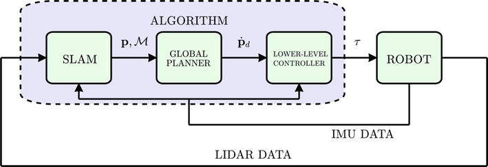
Figure 1.

Schematics of the algorithm.

More concretely, the contributions of this chapter include the use of CBFs with additional QP constraints to yield collision-free velocity commands. By keeping the outputs of the algorithm vehicle agnostic, the algorithm can be applied to any platform.

1.4 Organization

In Sections 2–4 the three modules displayed in Figure 1 are discussed. Then, in Section 5 simulation studies in the Gazebo environment showcase the algorithm’s operation. Finally, in Section 6 we give our concluding remarks.

2. Simultaneous localization and mapping (SLAM) module

The indoor navigation sensor suite is comprised of a 3D LiDAR sensor, attached on top of the UAV, as shown in Figure 2, an Inertial Measurement Unit (IMU) on the flight controller, and a downward-facing rangefinder placed underneath the UAV. The addition of the rangefinder provides a robust estimate of absolute distance to the ground since the LiDAR sensor is not expected to sense the floor due to its placement on the top of the vehicle.

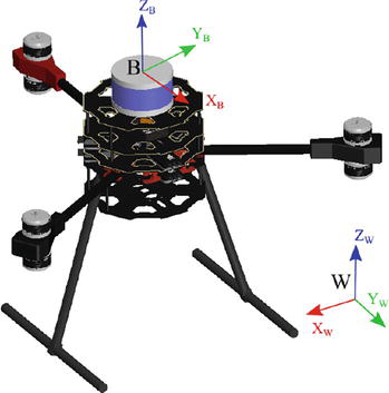
Figure 2.

Depiction of UAV agent with relevant coordinate frames.

The LiDAR point cloud and corresponding IMU measurements are fed to the FAST-LIO algorithm [32], which estimates odometry in a tightly-coupled iterated extended Kalman filter by fusing 3D feature points from LiDAR and measurements from IMU. Odometry from FAST-LIO is reliable for orientation and motion on the $\mathit{xy}$-plane.

An extended Kalman filter (EKF) [33] fuses IMU linear accelerations and angular velocities, rangefinder relative height measurements, and LiDAR-inertial odometry, resulting in an estimate of the UAV state. Let a world-fixed inertial frame be $\mathcal{W}$ and a body-fixed frame be $\mathcal{B}$ on the UAV IMU. Then the UAV’s state, as maintained at the EKF, is $\chi ={\left[{\mathbf{q}}^{\mathrm{T}}{\dot{\mathbf{q}}}^{\mathrm{T}}{\mathtt{F}}^{\mathrm{T}}\right]}^{\mathrm{T}},$ where $\mathbf{q}={\left[xyz\right]}^{\mathrm{T}}$ the UAV’s 3D-position in $\mathcal{W}$ and $\mathtt{F}={\left[\varphi \theta \psi \right]}^{\mathrm{T}}$ the roll, pitch, and yaw Euler angles of the UAV respectively.

Odometry estimates of the UAV are used as the basis for 3D occupancy grid mapping. Poses of LiDAR sensor measurements are integrated into a 3D occupancy grid map ${\overline{\mathcal{M}}}^{3D}\subseteq {\mathbb{R}}^3\times \left[0,1\right]$ with OctoMap [34] as its backbone. OctoMap framework stores the probability of occupancy of a 3D grid with an arbitrary size efficiently in an octree data structure. Let $\mathcal{Z}\left(t\right)=\left\{{}^L\mathbf{r}\in {\mathbb{R}}^3\right\}$ be the point cloud of LiDAR measurement at time $t$, corrected for the motion of the sensor and expressed in the frame coinciding with sensor’s origin, and ${\mathbf{T}}_L=\left[\begin{array}{cc}{\mathbf{R}}_L& {\mathbf{q}}_L\\ {\mathbf{0}}_{1\times 3}& 1\end{array}\right]\in \mathit{SE}\left(3\right)$ be the pose of the LiDAR sensor in the world frame, with ${\mathbf{R}}_L\in \mathit{SO}\left(3\right)$ denoting a rotation matrix and ${\mathbf{q}}_L\in {\mathbb{R}}^3$ as the origin of the sensor. Probability of occupancy is reduced for every grid cell in ${\overline{\mathcal{M}}}^{3D}$ that lie in the line defined as

$$\mathbf{l}\left(d\right)\triangleq {\mathbf{q}}_L+d\frac{{{\mathbf{R}}_L}^L\mathbf{r}}{\Vert {{\mathbf{R}}_L}^L\mathbf{r}\Vert };0\le d\le min\left(\Vert {{\mathbf{R}}_L}^L\mathbf{r}\Vert ,d_{\max }\right)$$E1

If the point is within a certain distance from the sensor origin, denoted as $d_{\max }$, then the probability of occupancy of the grid cell containing the endpoint is increased. The reason for including a maximum distance is mainly for efficiency purposes, as ray casting every point in $\mathcal{Z}\left(t\right)$ at every time step is an expensive process.

Instead of working with pure probabilities, the maximum likelihood estimate of the map ${\overline{\mathcal{M}}}^{3D}$ is obtained to classify the map into three distinct classes: occupied (1), free (−1), and unknown (0). The maximum likelihood map is denoted as ${\mathcal{M}}^{3D}\subseteq {\mathbb{R}}^3\times \left\{-\mathrm{1,0,1}\right\}$. Let the function $\mathit{\text{Class}}:{\mathbb{R}}^3\to \left\{-\mathrm{1,0,1}\right\}$ provide the class information for points in the 3D occupancy map.

For a continuous mapping mission with insufficient feature variety in an environment, a loop closure module to account for odometry drifts may be required. Minuscule errors in pose estimation via visual or visual-inertial odometry accumulate to introduce large inconsistencies. However, the odometry estimation obtained via the aforementioned EKF formulation provides sufficient accuracy for an indoor environment. Indoor spaces are seldom larger than the coverage a commercial 3D LiDAR sensor can provide. Therefore, a loop closure module is omitted, and the odometry estimates are relied on solely for mapping. However, it is possible to implement a 3D map-based loop closure module, similar to the vision-based approaches [35] using an equivalent global descriptor for depth data [36].

In this work, the navigation requirements of the UAV are limited to 2D. As such, only the occupancy of a subset of the 3D grid in ${\mathcal{M}}^{3D}$ that lies within a height range $z\in \left[h_{\min },h_{\max }\right]$ is of importance. To consolidate the information contained in the given height range, the occupancy information is reduced to a 2D grid via the projection of each point coordinate onto $\mathit{xy}$-plane. More concretely, let the coordinates of an arbitrary grid center in $\mathcal{M}$ be denoted as ${\mathbf{g}}_i={\left[x_i{y}_i\right]}^{\mathrm{T}}$, and the set of grid centers with the same $\mathit{xy}$-coordinates in ${\mathcal{M}}^{3D}$ be denoted as ${\mathbf{r}}_i\left(z\right)={\left[\begin{array}{ccc}{x}_i& y_i& z\end{array}\right]}^{\mathrm{T}}$. Note that the $\mathit{xy}$-coordinates of the points are shared between ${\mathbf{g}}_i$ and ${\mathbf{r}}_i\left(z\right)$. We defined the projection function $\mathit{\text{Proj}}:{\mathbb{R}}^2\to \left\{-\mathrm{1,0,1}\right\}$ as

$$\mathit{\text{Proj}}\left({\mathbf{g}}_i\right)\triangleq \left\{\begin{array}{ll}1& \exists {\mathbf{r}}_i\left(z\right)\in {\mathcal{M}}^{3D},z\in \left[h_{\min },h_{\max }\right],\mathit{\text{Class}}\left({\mathbf{r}}_i\left(z\right)\right)=1\\ -1& \forall {\mathbf{r}}_i\left(z\right)\in {\mathcal{M}}^{3D},z\in \left[h_{\min },h_{\max }\right],\mathit{\text{Class}}\left({\mathbf{r}}_i\left(z\right)\right)=-1\\ 0& \text{otherwise}.\end{array}\right.$$E2

The projection function given in (2) is conservative: the 2D coordinates are considered occupied even if a single point in the column of all points within the given height range is occupied, and the cell is considered free only if all of the points in the same column are free.

An example projection from a 3D map to a 2D map is provided in Figure 3(a). On the left is the binary OctoMap occupancy representation of the environment, color-coded based on the obstacle height. Upon projecting a height range of the map onto a 2D plane, the map representation on the right is obtained. Occupied, free, unknown, and frontier cells are represented in red, green, black, and magenta colors, respectively.

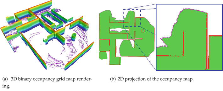
Figure 3.

A 3D rendering of the occupancy grid view, denoting the occupied cells with color coding, along with a sample 2D projection of the occupancy map. Occupied, free, unknown, and frontier cells are depicted in red, green, black, and magenta colors respectively. A zoomed-in view of the 2D occupancy map is provided for clarity.

3. “Global planner” module

Important concepts and subroutines will be clarified prior to the motion planning algorithm.

3.1 Map and distance functions

For the motion planning, the map $\mathcal{M}$ implies a collection of points ${\mathbb{R}}^2$ that represent the geometry of the environment detected so far using the LiDAR sensor. As this information evolves as the drone navigates the environment, it changes continuously, the term $\mathcal{M}\left(t\right)$ emphasizes the map up to a specific time $t$.

It is essential for the motion planning algorithm to compute distances between the drone and the map in order to plan a safe path. Furthermore, distance gradients are also necessary for the approach. Before considering the geometry of the robot, we will be concerned with the distance between a point $\mathbf{p}\in {\mathbb{R}}^2$ and an obstacle. Since we have a collection of points $\mathcal{M}\subseteq {\mathbb{R}}^2$, described as $\mathbf{g}$, a first idea is to compute the point-to-map distance $E_P\left(\mathbf{p}|\mathcal{M}\right)$ as the minimum Euclidean distance between $\mathbf{p}$ and the points $\mathbf{g}$. However, there is an issue with this approach: the function $E_P\left(\mathbf{p}|\mathcal{M}\right)$ is not differentiable in $\mathbf{p}$ due to two reasons: the fact that the individual Euclidean distances $\parallel \mathbf{p}-\mathbf{g}\parallel$ are non-differentiable on $\mathbf{p}$ and also the fact the minimum function is non-differentiable at some points. The first issue can be easily solved by using the squared Euclidean distance $\parallel \mathbf{p}-\mathbf{g}{\parallel }^2$, and the second can be addressed by using an approximated version of the minimum that can be guaranteed to be differentiable. The softmin function [37] is a good candidate, defined (with an averaging term) as

$$\stackrel{h}{min}\left(g_1,g_2,\dots ,g_m\right)\triangleq -hln\left(\frac{1}{m}\sum _{k=1}^{m}exp\left(-\frac{g_k}{h}\right)\right).$$E3

This function is always differentiable in the arguments $g_i$ and approximates the minimum when $h$ is positive and close to 0. With softmin as the minimum, the point-to-map squared distance is defined

$$E_P\left(\mathbf{p}|\mathcal{M}\right)\triangleq \underset{\mathbf{g}\in \mathcal{M}}{\overset{h}{min}}\parallel \mathbf{p}-\mathbf{g}{\parallel }^2$$E4

in which $h$ is a parameter. With this definition, the gradient of $E_P\left(\mathbf{p}|\mathcal{M}\right)$ is computed as

$${\nabla }_{\mathbf{p}}{E}_P\left(\mathbf{p}|\mathcal{M}\right)=\mathbf{p}-\frac{{\sum }_{\mathbf{g}\in \mathcal{M}}exp\left(-\parallel \mathbf{p}-\mathbf{g}{\parallel }^2/h\right)\mathbf{g}}{{\sum }_{\mathbf{g}\in \mathcal{M}}exp\left(-\parallel \mathbf{p}-\mathbf{g}{\parallel }^2/h\right)}.$$E5

The drone is modeled by a sphere of radius $R_{\mathit{ROB}}$. Thus, using the previously-defined point-to-map distance, the robot-to-map squared distance is defined as $E\left(\mathbf{p}|\mathcal{M}\right)\triangleq E_P\left(\mathbf{p}|\mathcal{M}\right)-R_{\mathit{ROB}}^2$, in which $\mathbf{p}\in {\mathbb{R}}^2$ given by $\mathbf{p}={\left[xy\right]}^{\mathrm{T}}$ is the drone’s 2D position. Note that this is different than $\mathbf{q}={\left[xyz\right]}^{\mathrm{T}}$ introduced in the previous section: $\mathbf{p}$ is the projection of $\mathbf{q}$ in a plane parallel to the ground. Since the planner is 2D only, it does not require the height $z$. Nevertheless, we can easily compute the gradient of this function as ${\nabla }_{\mathbf{p}}E\left(\mathbf{p}|\mathcal{M}\right)={\nabla }_{\mathbf{p}}{E}_P\left(\mathbf{p}|\mathcal{M}\right)$, in which ${\nabla }_{\mathbf{p}}{E}_P\left(\mathbf{p}|\mathcal{M}\right)$ is computed according to (5).

3.2 Control barrier functions with circulation constraints

The utilized global planner needs a local planner that plans a (usually short) path from one point to another while avoiding obstacles. It is common to plan using a straight line, and the planner is successful if this line does not cross any obstacle within a safety margin. Although this strategy is simple to implement, it may be inefficient because the path may be often blocked by obstacles, requiring many calls to the local planner until a path (formed by line segments) is found. We will propose another approach that, although not as simple to implement as a straight line, provides successful paths more often because it is able to deviate from the obstacles.

Suppose the existence of a point $\mathbf{p}$ in which its velocity $\dot{\mathbf{p}}=\mathbf{u}$ is controlled. This control input $\mathbf{u}$ should guide $\mathbf{p}$ from its starting position to a final position ${\mathbf{p}}_G\in {\mathbb{R}}^2$, while avoiding collision with the map $\mathcal{M}$. During the planning phase starting at time $t_0$, the map $\mathcal{M}\left(t\right)$ is assumed to be constant, being $\mathcal{M}\left(t_0\right)$.

$\dot{\mathbf{p}}$ is computed using control barrier functions with circulation constraints [29]. At each point $\mathbf{p}$ the velocity $\mathbf{u}\left(\mathbf{p}\right)$ is computed by solving a QP problem that guides the point towards the target while avoiding obstacles. This QP has two constraints: one directly from the CBF, and another derived from it, that induces a circulation behavior. The circulation behavior is a novelty introduced in [29] that helps deviate from obstacles with a negligible increase in the cost of the algorithm.

The following parameters of this formulation are defined:

• Let $\mathrm{\Omega }\in {\mathbb{R}}^{2\times 2}$ be a skew-symmetric matrix, that determines how the environment is circulated;

• Let $\alpha :\mathbb{R}\mapsto \mathbb{R}$ be a continuous, decreasing function with $\alpha \left(0\right)=0$, that determines how fast obstacles can be approached given how close are;

• Let $\beta :\mathbb{R}\mapsto \mathbb{R}$ be a continuous, decreasing function such with $\beta \left(0\right)>0$ and $\beta \left(E\left({\mathbf{p}}_G|\mathcal{M}\right)\right)<0$, that determines how much an obstacle is forced to be circulated given how close to it the robot is.

• Let $K_C$ be a positive constant that determines the approach speed to the target.

Furthermore, define the normal and tangent vectors:

$$\mathbf{N}\left(\mathbf{p}\right)\triangleq \frac{{\nabla }_{\mathbf{p}}E\left(\mathbf{p}|\mathcal{M}\right)}{\parallel {\nabla }_{\mathbf{p}}E\left(\mathbf{p}|\mathcal{M}\right)\parallel }\text{and}\mathbf{T}\left(\mathbf{p}\right)\triangleq \frac{\mathrm{\Omega }{\nabla }_{\mathbf{p}}E\left(\mathbf{p}|\mathcal{M}\right)}{\parallel \mathrm{\Omega }{\nabla }_{\mathbf{p}}E\left(\mathbf{p}|\mathcal{M}\right)\parallel }$$E6

Both are well defined (i.e ${\nabla }_{\mathbf{p}}E\left(\mathbf{p}|\mathcal{M}\right)$ and $\mathrm{\Omega }{\nabla }_{\mathbf{p}}E\left(\mathbf{p}|\mathcal{M}\right)$ are non-null vectors). Finally, define ${\mathbf{u}}_d\left(\mathbf{p}\right)\triangleq -K_C\left(\mathbf{p}-{\mathbf{p}}_G\right)$. Then the CBF + QP formulation to compute $\mathbf{u}\left(\mathbf{p}\right)$ is as follows [29]:

$$\mathbf{u}\left(\mathbf{p}\right)=arg\underset{\mu }{min}\parallel \mu -{\mathbf{u}}_d\left(\mathbf{p}\right){\parallel }^2$$E7

$$\text{such}\text{that}:\mathbf{N}{\left(\mathbf{p}\right)}^{\mathrm{T}}\mu \ge \alpha \left(E\left(\mathbf{p}|\mathcal{M}\right)\right)$$E8

$$\mathbf{T}{\left(\mathbf{p}\right)}^{\mathrm{T}}\mu \ge \beta \left(E\left(\mathbf{p}|\mathcal{M}\right)\right).$$E9

This is a QP problem that always has a solution, and furthermore, this solution is unique because it is a strictly convex problem. Care must be taken when the problem is not well defined. This can be divided into three mutually exclusive conditions:

• $\mathrm{\Omega }{\nabla }_{\mathbf{p}}E=\mathbf{0}$ but ${\nabla }_{\mathbf{p}}E\cancel{=}\mathbf{0}$. In this case, we just discard the tangent constraint. This is especially important because $\mathrm{\Omega }$ being the $2\times 2$ null matrix is a possibility.

• ${\nabla }_{\mathbf{p}}E=\mathbf{0}$ and $E>0$. In this case, we can disregard the normal and tangential constraints and just use $\mathbf{u}\left(\mathbf{p}\right)={\mathbf{u}}_d\left(\mathbf{p}\right)$.

• ${\nabla }_{\mathbf{p}}E=\mathbf{0}$ and $E\le 0$. In this case, we have to stop, since we do not have distance gradient information and we are dangerously close to obstacles.

The planner can fail in three different cases: (i) because the third condition is reached, (ii) because the robot has reached a point in which $\mathbf{u}\left(\mathbf{p}\right)=\mathbf{0}$ but $\mathbf{p}\ne {\mathbf{p}}_G$ or (iii) because a limit cycle has been reached.

3.3 Local planner function

With the description given in the previous subsection, we can define the CBFCircPlanOne function:

$$\left(\mathcal{P},S\right)\leftarrow \mathtt{\text{CBFCircPlanOne}}\left({\mathbf{p}}_0,{\mathbf{p}}_G,\mathcal{M},\mathrm{\Omega },T\right)$$E10

which is at the core of the motion planning algorithm. It takes as arguments a starting point ${\mathbf{p}}_0\in {\mathbb{R}}^2$, a goal point ${\mathbf{p}}_G\in {\mathbb{R}}^2$, a map $\mathcal{M}$, a circulation $\mathrm{\Omega }$ and a time period $T$, and tries, using the procedure described in the previous subsection, to plan a collision-free path from ${\mathbf{p}}_0$ to ${\mathbf{p}}_G$ while avoiding the obstacles detected in the map and using as a circulation parameter $\mathrm{\Omega }$, while integrating the dynamical system $\dot{\mathbf{p}}=\mathbf{u}\left(\mathbf{p}\right)$ from $t=0$ to $t$ at most $T$ time units. Note that the algorithm can halt before it reached $t=T$ in the integration, either because it detects one of the failure conditions described in the previous subsection or because it reached the goal. Nevertheless, it returns the path $\mathcal{P}$ it obtained until it halted and also a signal $S\in \left\{\mathit{\text{TRUE}},\mathit{\text{FALSE}}\right\}$ saying if it was successful or not. Naturally, the resulting differential equation cannot be solved analytically except in very simple cases, and the path is computed using a numerical integration scheme. Related to this function, we define the CBFCircPlanMany function:

$$\left(\mathcal{P},{\mathrm{\Omega }}_{\mathit{\text{BEST}}},S\right)\leftarrow \mathtt{\text{CBFCircPlanMany}}\left({\mathbf{p}}_0,{\mathbf{p}}_G,\mathcal{M},T\right)$$E11

which plans many paths from ${\mathbf{p}}_0$ to ${\mathbf{p}}_G$, with the map $\mathcal{M}$ and with each one of them integrating until at most $t=T$, using different previously-defined rotations $\mathrm{\Omega }$. Thus, this function calls CBFCircPlanOne many times. It returns the shortest path $\mathcal{P}$ among all the successful paths, the best circulation matrix ${\mathrm{\Omega }}_{\mathit{\text{BEST}}}$ that achieved this smallest successful path and a signal $S\in \left\{\mathit{\text{TRUE}},\mathit{\text{FALSE}}\right\}$ saying if at least one of the paths was successful or not. In the proposed approach, three different matrices $\mathrm{\Omega }$ were used, representing clockwise rotation, counter-clockwise rotation, and a non-rotation. More precisely, let

$${\mathrm{\Omega }}_Z\triangleq \left(\begin{array}{cc}0& -1\\ 1& 0\end{array}\right),{\mathrm{\Omega }}_0\triangleq \left(\begin{array}{cc}0& 0\\ 0& 0\end{array}\right)$$E12

then $+{\mathrm{\Omega }}_Z$ (counter-clockwise), $-{\mathrm{\Omega }}_Z$ (clockwise) and ${\mathrm{\Omega }}_0$ (no induced rotation) is used.

3.4 Vector field path tracking

The global planner periodically revises its plan and eventually commits the drone to a path $\mathcal{P}$. Once a path is given, the robot’s low-level control input is computed - its linear velocity (see Section 4) - to track this path. For this, the vector field methodology is used [30]. The function $\dot{\mathbf{p}}\leftarrow \mathtt{\text{vectorField}}\left(\mathbf{p},\mathcal{P}\right)$ will return the linear velocity $\dot{\mathbf{p}}$ to be sent to the lower level controllers given the current position $\mathbf{p}$ and the committed path $\mathcal{P}$.

3.5 Exploration graph generation

In order to run the motion planning algorithm, as the drone moves, a graph $\mathcal{G}$ is incrementally generated that represents the connectivity of the environment in a simplified and structured way when compared to the map $\mathcal{M}$. Each “node” $N$ of the graph is associated with a position in the map. Two nodes/points ${\mathbf{p}}_A$ and ${\mathbf{p}}_B$ are connected if and only if a safe path is secured between ${\mathbf{p}}_A$ and ${\mathbf{p}}_B$. As this graph is updated/built as the drone moves, it is also time-variant, described by $\mathcal{G}\left(t\right)$.

Associated with this graph, the following functions can be found:

• ${\mathcal{G}}^{\prime }\leftarrow \mathtt{\text{updateGraph}}\left(\mathbf{p},\mathcal{G},\mathcal{M}\right)$, which updates the current graph $\mathcal{G}$, given the current position $\mathbf{p}$ and the current known map $\mathcal{M}$, returning the updated graph ${\mathcal{G}}^{\text{'}}$. It tries to insert a new node associated with the current position $\mathbf{p}$ by trying to connect this node to another one already on $\mathcal{G}$ (the closest one in which the connection is possible), taking into consideration the obstacles codified into the map $\mathcal{M}$. The graph is undirected and weighted by the distance between the two nodes.

• $\mathcal{N}\leftarrow \mathtt{\text{getNearestNodes}}\left(\mathbf{p},\mathcal{G}\right)$ returns a sorted list of all the nodes $\mathcal{N}$ of the graph $\mathcal{G}$ sorted by their Euclidean distance to the point $\mathbf{p}$ in ascending order.

• $\left(N,L\right)\leftarrow \mathtt{\text{getNearestReachableNode}}\left(\mathbf{p},\mathcal{G},\mathcal{M}\right)$ returns a node $N$ of the graph $\mathcal{G}$ such that there is a path from $\mathbf{p}$ to $N$, considering the obstacles codified into $\mathcal{M}$. It also returns the length $L$ of this path. This function can be implemented as follows: getNearestNodes is used to get a list of nodes, sorted by the Euclidean distance to $\mathbf{p}$. Then CBFCircPlanMany is used in each one of them until the planner is successful. The first successful node is returned as $N$. The assumption is that this algorithm never fails, i.e., the graph $\mathcal{G}$ is a good enough representation of the map $\mathcal{M}$ and the local planner is good enough to always move from the current position to one of the nodes of the graph.

• $\left(\mathcal{N},L\right)\leftarrow \mathtt{\text{getPath}}\left(N_A,N_B,\mathcal{G}\right)$ returns a list of nodes $\mathcal{N}$ containing the shortest path from node $N_A$ to node $N_B$ given the graph $\mathcal{G}$, and also the length (sum of the weights between the edges) of this path. This shortest path considers only the weights codified into the edges of the graph, does not take into consideration the map $\mathcal{M}$, and can be computed using (for example) Dijkstra’s algorithm. Note that, given the nature of the graph building scheme described here, such a path always exists between two given nodes, since it only adds a node to the graph (using the updateGraph function) if a path between that node and another node (already in the graph) exists.

3.6 Frontier points and frontier exploration

Eventually, the motion planner should request the robot to go to an unexplored region of the map [33]. For this, a function $\mathcal{F}\leftarrow \mathtt{\text{getAllFrontiers}}\left(\mathcal{M}\right)$ is implemented that obtains a set of representative frontier points $\mathcal{F}$ from the currently-known map $\mathcal{M}$.

A frontier point is defined as a coordinate in 2D binary occupancy map $\mathcal{M}$ which is classified as a free cell, is in the 8-neighborhood of a cell that is marked unknown, and is not in the 8-neighborhood of a cell that is marked occupied. To this end, standard image processing tools are utilized by treating the 2D binary occupancy as a binary image with 2 channels (maps): an occupied channel, denoted $\mathit{Oc}:{\mathbb{N}}^2\to \left\{0,1\right\}$, with pixel value of 1 if the coordinate is occupied, and a free channel, denoted as $\mathit{Fr}:{\mathbb{N}}^2\to \left\{0,1\right\}$, whose coordinates take the value 1 for free coordinates. Due to the definition of the projection as given in (2), a coordinate cannot have both values in the two channels be 1. Implicitly, any coordinate at which both channels have a 0 value is unknown.

The occupied channel $\mathit{Oc}$ is firstly dilated by 1 pixel to obtain the image $\overline{O}c$. Then the internal and external contours of the free channel $\mathit{Fr}$ are extracted, denoted as $\mathcal{C}\subseteq {\mathbb{N}}^2$. For every contour point $\mathbf{g}$, the corresponding value in $\overline{O}c$ is checked at the pixel coordinate given by $\mathbf{g}$. All the points $\mathbf{g}\in \mathcal{C}$ that have a 0 value in $\overline{O}c$ constitute the frontier, $\mathcal{F}$. More concretely:

$$\mathcal{F}=\left\{\mathbf{g}\in \mathcal{C},\overline{O}c\left(\mathbf{g}\right)=0\right\}.$$E13

A sample of frontier points is marked in Figure 3(b), which can be seen as the magenta points in the zoomed-in view.

Once these points are obtained, an algorithm decides which point it is going to explore next. This is achieved by function $\left\{\mathcal{N},S\right\}\leftarrow \mathtt{\text{selectExplorationFrontier}}\left(\mathbf{p},\mathcal{M},\mathcal{F},\mathcal{G}\right)$ that processes the current position $\mathbf{p}$, the current map $\mathcal{M}$, the frontier points $\mathcal{F}$ and the graph $\mathcal{G}$, and returns the path one should travel from the points of the graph $\mathcal{G}$ to reach one of the frontier points (if one is found) and a signal $S\in \left\{\mathit{\text{TRUE}},\mathit{\text{FALSE}}\right\}$ if it was successful.

The algorithm’s structure is:

• Step 1: For each point ${\mathbf{p}}_F\in \mathcal{F}$ the CBFCircPlanMany function is used to try to connect $N_{\mathit{TRY}}$ (a parameter) different nodes of $\mathcal{G}$ to the point ${\mathbf{p}}_F$. The $N_{\mathit{TRY}}$ closest nodes from ${\mathbf{p}}_F$, obtained from the getNearestNodes functions are tried. The points in which it was not possible to connect none of these $N_{\mathit{TRY}}$ nodes to ${\mathbf{p}}_F$ are discarded, meaning that these frontier points are most likely unreachable, obtaining a new set ${\mathcal{F}}^{\text{'}}\subseteq \mathcal{F}$. For each point in ${\mathbf{p}}_F\in {\mathcal{F}}^{\text{'}}$, this procedure also allows us to create two maps: $N\leftarrow \mathtt{\text{closestSuccesfulNode}}\left[{\mathbf{p}}_F\right]$ that maps the frontier point into the node $N$ of the graph $\mathcal{G}$ that has the shortest successful path from it, and $L\leftarrow \mathtt{\text{shortPathLengthFromGraphToFrontier}}\left[{\mathbf{p}}_F\right]$ that gives the length of this shortest successful path.

  • If ${\mathcal{F}}^{\text{'}}=\varnothing$, the algorithm ends, since most likely anything anymore can be explored.

  • Otherwise, proceed to Step 2.

• Step 2: For each one of the positions in ${\mathbf{p}}_F\in {\mathcal{F}}^{\text{'}}$, the CBFCircPlanMany function is used to try to connect this point to the global target ${\mathbf{p}}_{\mathit{\text{GLOBAL}}}$. Those points in which we were successful are aggregated into a set ${\mathcal{F}}^{″}$, and this procedure allows us to create a map $L\leftarrow \mathtt{\text{shortPathLengthFromFrontierToGoal}}\left[{\mathbf{p}}_F\right]$ with this smallest length.

  • If ${\mathcal{F}}^{″}\cancel{=}\varnothing$, proceed to Step 3.

  • Otherwise, proceed to Step 4.

• Step 3: For each one of the positions in ${\mathbf{p}}_F\in {\mathcal{F}}^{″}$, a metric is computed that decides which point is going to be explored. This metric is given by the sum of

  • The path length $L_p^{\mathit{\text{GStart}}}$ from $\mathbf{p}$ to a node $N_{\mathit{\text{GStart}}}$ in the graph, obtained from $\left(N_{\mathit{\text{GStart}}},L_p^{\mathit{\text{GStart}}}\right)\leftarrow \mathtt{\text{getNearestReachableNode}}\left(\mathbf{p},\mathcal{G},\mathcal{M}\right)$;

  • The path length $L_{\mathit{\text{GStart}}}^{\mathit{\text{GEnd}}}$ from $N_{\mathit{\text{GStart}}}$ to the node $N_{\mathit{\text{GEnd}}}=\mathtt{\text{closestSuccesfulNode}}\left[{\mathbf{p}}_F\right]$, obtained from getPath $\left(N_{\mathit{\text{GStart}}},N_{\mathit{\text{GEnd}}}\right)$;

  • The path length $L_{\mathit{\text{GEnd}}}^F$ from $N_{\mathit{\text{GEnd}}}$ to the frontier point ${\mathbf{p}}_F$ using the shortest planned path, which is $L_{\mathit{\text{GEnd}}}^F=\mathtt{\text{shortPathLengthFromGraphToFrontier}}\left[{\mathbf{p}}_F\right]$;

  • The path length $L_F^{\mathit{\text{GLOBAL}}}$, which is

    $$L_F^{\mathit{\text{GLOBAL}}}=\mathtt{\text{shortPathLengthFromFrontierToGoal}}\left[{\mathbf{p}}_F\right].$$

    The point ${\mathbf{p}}_F$ is returned with the smallest such metric, the list of nodes from $N_{\mathit{\text{GStart}}}$ and $N_{\mathit{\text{GEnd}}}$ as $\mathcal{N}$, together with a dummy node at the end (that is not on $\mathcal{G}$) that represents the frontier point ${\mathbf{p}}_F$, and thus the algorithm ends. This metric is an estimate of how long the optimistic path from the current point $\mathbf{p}$ to the global target ${\mathbf{p}}_{\mathit{\text{GLOBAL}}}$ is, assuming that the current map is the final map, and thus the most promising frontier points are selected to explore;

• Step 4: If ${\mathcal{F}}^{″}=\varnothing$, Step 3 is reproduced but with ${\mathcal{F}}^{\prime }$ instead of ${\mathcal{F}}^{″}$ and without the last term, $L_F^{\mathit{\text{GLOBAL}}}$ (since it was not possible to plan a path from the frontier to the goal).

3.7 The motion planning algorithm

With all the necessary functions introduced, the motion planning algorithm can be explained. Let the state variables of the planner, be internal variables that must be stored all the time and that are read and modified by the flow of the algorithm:

• The current committed path ${\mathcal{P}}_C$ that the vector field algorithm needs to follow, which is empty in the beginning.

• The current graph $\mathcal{G}$, starting with a graph with a single node, representing the starting position ${\mathbf{p}}_0$;

• The current rotation parameter $\mathrm{\Omega }$. This can be initialized as any one of the three possible rotations described in (12) (e.g: ${\mathrm{\Omega }}_0$);

• The current goal ${\mathbf{p}}_G$, which starts with the global goal ${\mathbf{p}}_{\mathit{\text{GLOBAL}}}$;

• The current navigation mode $V$, that can be either goingToGlobal or goingToFrontier. It starts with goingToGlobal;

• The current list of nodes from $\mathcal{G}$ that we should track, ${\mathcal{N}}_C$, along with the current node on this list, $N_C\in \mathcal{N}$. These two states are only used when $V=\mathtt{\text{goingToFrontier}}$, and since $V$ starts with goingToGlobal, it does not matter how they are initialized.

As shown in Figure 1, the inputs of the algorithm are the current position $\mathbf{p}$ and map $\mathcal{M}$ from the SLAM algorithm, and the output is the desired linear velocity ${\dot{\mathbf{p}}}_d$ to be provided to the lower level controller. It has three different sub-algorithms, labeled as A, B, and C, that runs in different frequencies (and the latter asynchronously as well) and reads and modifies the state variables.

In a given frequency $f_A$—which is the frequency in which the algorithm is going to output the linear velocity—the planner uses the vector field algorithm to track the committed path ${\mathcal{P}}_C$, providing $\dot{\mathbf{p}}$, and also check if the current target ${\mathbf{p}}_G$ was reached. In a frequency $f_B<f_A$, it replans the committed path ${\mathcal{P}}_C$ based on the current goal ${\mathbf{p}}_G$, and, finally, in a frequency $f_C<f_B$, it updates the graph, replans the goal ${\mathbf{p}}_G$ itself, the current $\mathrm{\Omega }$ and the current navigation mode $V$.

A more detailed description of each sub-algorithm is shown in the sequel:

• Algorithm A: running at a frequency $f_A$. This algorithm is responsible to verify if the target was achieved, changing the flow of the algorithm if it is the case. It may call Algorithm C below. It also sends commands to the lower-level controller.

  • Step 1.A: Check whether the current goal is reached by checking if $\parallel \mathbf{p}-{\mathbf{p}}_G\parallel \le \delta$ for a parameter $\delta$.

    1. If this is false, go to Step 2.A;

    2. If this is true and V==goingToGlobal, the mission is accomplished and the whole algorithm ends.

    3. If this is true and V==goingToFrontier, check whether the node $N_C$ is the last on the list ${\mathcal{N}}_C$, or not.

       1. If not, set $N_C$ to the next of the list and set $\mathbf{p}G\leftarrow N_C$. Call Algorithm C and, when it halts, go to Step 2.A.

       2. If it was the last node of the list, set V $\leftarrow$ goingToGlobal, set $\mathbf{p}G\leftarrow \mathbf{p}\mathit{\text{GLOBAL}}$. Call Algorithm C and, when it halts, go to Step 2.A.

  • Step 2.A: compute ${\dot{\mathbf{p}}}_d\leftarrow \mathtt{\text{vectorField}}\left(\mathbf{p},{\mathcal{P}}_C\right)$ and output it to the lower level controller. Algorithm A then ends.

• Algorithm B: running at a frequency $f_B$. This algorithm is responsible for updating the path that is being tracked. It consists of a single step, running

  $$\left({\mathcal{P}}_C,S\right)\leftarrow \mathtt{\text{CBFCircPlanOne}}\left({\mathbf{p}}_0,{\mathbf{p}}_G,\mathcal{M},\mathrm{\Omega },T_B\right)$$E14

  for a fixed time $T_B$ (a parameter), updating ${\mathcal{P}}_C$. Irrelevant on whether it failed or not, since it is a small local path that is unlikely to reach the current target unless the drone is very close to it. Thus, disregard S. Algorithm B then ends.

• Algorithm C: running at a frequency $f_C$, and asynchronously (when called by Algorithm A). It is responsible to replan the target ${\mathbf{p}}_G$ and also updating the graph.

  • Step 1.C: Run $\mathcal{G}\leftarrow \mathtt{\text{updateGraph}}\left(\mathbf{p},\mathcal{G},\mathcal{M}\right)$ to update the graph. Go to Step 2.C.

  • Step 2.C: Replan the path to the current goal by running

    $$\left(\mathcal{P},{\mathrm{\Omega }}_{\mathit{\text{BEST}}},S\right)\leftarrow \mathtt{\text{CBFCircPlanMany}}\left(\mathbf{p},{\mathbf{p}}_G,\mathcal{M},T_C\right)$$E15

    for a fixed time $T_C$ (a parameter).

    • If the algorithm was a success (S==TRUE), set $\mathrm{\Omega }\leftarrow {\mathrm{\Omega }}_{\mathit{\text{BEST}}}$ and Algorithm C ends (do not care about $\mathcal{P}$).

    • If the algorithm fails (S==FALSE), it means that very likely it is no use to try to go to the current target point ${\mathbf{p}}_G$, and there is no need to change it. Explore a frontier point, and thus run $\mathcal{F}\leftarrow \mathtt{\text{getAllFrontiers}}\left(\mathcal{M}\right)$, and then $\left\{{\mathcal{N}}_E,S\right\}\leftarrow$ $\mathtt{\text{selectExplorationFrontier}}\left(\mathbf{p},\mathcal{M},\mathcal{F},\mathcal{G}\right)$.

      • If S == TRUE, set $V\leftarrow$ goingToFrontier, ${\mathcal{N}}_C\leftarrow {\mathcal{N}}_E$, $N_C$ to the first node of ${\mathcal{N}}_C$, and ${\mathbf{p}}_G\leftarrow N_C$. Try to replan, going back to Step 2.C;

      • If S == FALSE, the whole algorithm ends with failure, because there is nothing to explore anymore and the global goal was not found;

4. “Low-level controller” module

Given the desired 2D linear velocity ${\dot{\mathbf{p}}}_d$ commanded by the global planner, this vector is augmented with a 0—since we want to maintain a constant height—at the end to obtain the 3D desired linear velocity ${\dot{\mathbf{q}}}_d$. The velocity controller computes a desired acceleration vector as

$${\alpha }_d=\mathbf{g}-K_p\left(\dot{\mathbf{q}}-{\dot{\mathbf{q}}}_d\right)-K_I{\int }_0^t\left(\dot{\mathbf{q}}-{\dot{\mathbf{q}}}_d\right)\mathit{d\tau },$$E16

where $K_p,K_I$ are positive gains and $\mathbf{g}={\left[\mathrm{0,0,9.81}\right]}^{\mathrm{T}}{\mathit{ms}}^{-2}$.

A low-level attitude controller runs on the UAV autopilot, relying on the ArduCopter firmware, controlling the vehicle’s orientation and commanding the signals to the motors. Using the vehicle mass $m$, the desired acceleration vector $\alpha$ is turned into thrust, roll, and pitch commands for the attitude controller as:

$$T=\frac{m{\alpha }_d^{\mathrm{T}}{\mathbf{e}}_3}{cos\left(\varphi \right)cos\left(\theta \right)},{\varphi }_d=-\frac{m{\alpha }_d^{\mathrm{T}}{\mathbf{e}}_1}{T},{\theta }_d=\frac{m{\alpha }_d^{\mathrm{T}}{\mathbf{e}}_2}{T}$$E17

where ${\mathbf{e}}_i$ is a unit vector along axis $i$. For the purposes of this work, the commanded yaw angle ${\psi }_d$ is always kept at zero.

The ArduCopter autopilot uses a cascade PID structure to transform the desired orientation commands into angular velocities and subsequently desired moments, which are combined with the desired thrust result into throttle level commands for the motors, which is the vector $\tau \in {\mathbb{R}}^4$ depicted into Figure 1. The structure of the low-level attitude controller is illustrated in Figure 4. The output of the motor mixer is PWM-values for the Electronic Speed Controllers of the UAV motors, controlling the speed of each motor. Current attitude $\mathrm{\Phi }$ is available from the EKF, while current angular rate $\dot{\mathrm{\Phi }}$ is provided directly by the gyroscope.

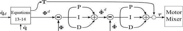
Figure 4.

Cascade PID structure of low-level attitude controller.

5. Simulation studies

To showcase the results of the algorithm, a warehouse-like Gazebo environment is used, depicted in Figure 5 in which the objective is to move from the starting position (magenta circle to the right) to the end position (green circle to the left). The goal is to go from a starting position ${\mathbf{p}}_0={\left[00\right]}^{\mathrm{T}}m$ to a global goal position ${\mathbf{p}}_{\mathit{\text{GLOBAL}}}={\left[-\mathrm{6.5,1.0}\right]}^{\mathrm{T}}m$, all written in a world-frame which is the starting body drone frame. The drone keeps a constant height value of $1.0m$. The parameters used were:

• For the map generation: Both FAST-LIO and OctoMap build their respective maps with a voxel grid size of $0.05m$. Furthermore, $d_{\max }$ that controls the range of updates on occupancy probabilities is set to $5.0m$.

• For the global planner: $h=0.07m^2$, $R_{\mathit{ROB}}=0.9m$, $K_C=0.50s^{-1}$, $N_{\mathit{TRY}}=5$, $f_A=100s^{-1}$, $f_B=5s^{-1}$, $f_C=0.5s^{-1}$, $T_B=2s$, $T_C=240s$, $\delta =0.13m$. Furthermore, $\alpha \left(E\right)$ was used such that $-A_{\mathit{POS}}\sqrt{E}$ when $E\ge 0$ and $A_{\mathit{NEG}}\sqrt{-E}$ when $E<0$ with $A_{\mathit{POS}}=0.05s^{-1}{m}^{-0.5}$ and $A_{\mathit{NEG}}=0.60s^{-1}{m}^{-0.5}$. Also, the function $\beta \left(E\right)=v_{\mathit{\text{CIRC}}}\left(1-E/D_{\mathit{\text{CIRC}}}^2\right)$ was employed with $v_{\mathit{\text{CIRC}}}=0.20{\mathit{ms}}^{-1}$ and $D_{\mathit{\text{CIRC}}}=0.32m$.

• For the UAV controllers: For the first stage PID (angle) the ArduCopter has $P=\left(\mathrm{11.6,12.0,5.4}\right)s^{-1}$ for roll, pitch, and yaw respectively with $0$ integral and derivative gains. For the second stage (angular rate) the gains were $P=\left(\mathrm{0.089,0.13,0.88}\right)s^{-1}$, $I=\left(\mathrm{0.08,0.078,0.088}\right)s^{-2}$, $D=\left(\mathrm{0.0024,0.004,0}\right)$ (dimensionless) respectively. For the velocity controller, the gains used were $K_p=0.5s^{-1}$, $K_I=0.05s^{-2}$. The mass of the UAV is $m=3.5\mathit{kg}$.

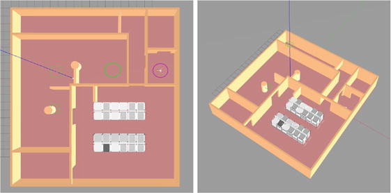
Figure 5.

Environment in two different perspectives.

Figures 6 and 7 show some snapshots of the algorithm at different times. Figure 7 also shows the graph $\mathcal{G}$ at the end of the algorithm. The drone’s current position is represented as a magenta circle, the target position ${\mathbf{p}}_{\mathit{\text{GLOBAL}}}$ as a green circle, the current goal ${\mathbf{p}}_{\mathit{\text{GOAL}}}$ as a red square, the points discovered so far as blue dots, the frontier points as gray dots, the current planned path with a red dashed line, the traced path in black. When the algorithm is in goingToFrontier mode, the graph nodes in orange and the selected frontier point ${\mathbf{p}}_F$ is represented by a black dot. Each one of the snapshots is further described:

• Figure 6 left-top: at the start, the drone is at gointToGlobal mode and, given the current map information (blue points), plan to go using a simple path (red dashed path) towards the global target (green start). Figure 6 right-top: the point is still at the same mode. Figure 6 left-middle: The robot still has hope to achieve the target. Figure 6 right-middle: after realizing that it cannot go to the global target, the drone decides that the best plan is to try to go from above since so far it did not discover that it is impossible to go from there. It changes the circulation mode and goes to the top, still in the gointToGlobal mode. Figure 6 left-bottom: after reaching the top, it realizes that it is blocked there as well: it is a dead-end. It decides to explore a frontier point (black dot) and enter the goingToFrontier mode to approach this point. Figure 6 right-bottom: after it travels all the nodes, it plans to go to the frontier point.

• Figure 7 left-top: the drone reaches the frontier point and switches back to the gointToGlobal, hoping to achieve the target given its current information of the map. Figure 7 right-top: eventually it realizes that it is not possible using the planned path. It plans to explore again. Figure 6 left-middle: it finds a point to explore and enters the goingToFrontier mode. Note that there are no orange points this time: the list of the nodes to be traveled only contains the frontier point ${\mathbf{p}}_F$, since the robot was already close to it. Figure 6 right-middle: it goes back to gointToGlobal, hoping to achieve the target given its current information on the map. Figure 6 left-bottom: the robot completed the mission successfully. Figure 6 right-bottom: graph structure $\mathcal{G}$ on the map.

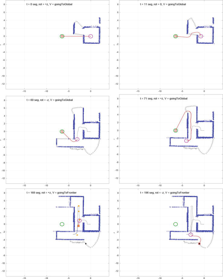
Figure 6.

Snapshots of the simulation.

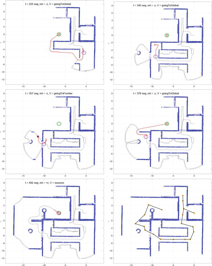
Figure 7.

Snapshots of the simulation and of the graph structure $\mathcal{G}$.

6. Conclusion

In this chapter, a framework is provided for the autonomous navigation of a drone in a GNSS-denied and unknown environment, aiming to reach a target point while avoiding obstacles and being equipped with only a LiDAR and IMU. The 2D-navigation algorithm is divided into three modules, that were discussed in detail. We showcased how the algorithm works through a Gazebo simulation physics engine, in which the simulated drone successfully navigated safely towards the goal.

Acknowledgments

This work was partially supported by the NYUAD Center for Artificial Intelligence and Robotics (CAIR), funded by Tamkeen under the NYUAD Research Institute Award CG010.

References

- 1.
Arvanitakis I, Tzes A, Giannousakis K. Synergistic exploration and navigation of mobile robots under pose uncertainty in unknown environments. International Journal of Advanced Robotic Systems. 2018; 15 (1):1729881417750785 - 2.
Ilyas M, Ali ME, Rehman N, Abbasi AR. Design, development & evaluation of a prototype tracked mobile robot for difficult terrain. Sir Syed University Research Journal of Engineering & Technology. 2013; 3 (1):7-7 - 3.
Tzes M, Papatheodorou S, Tzes A. Visual area coverage by heterogeneous aerial agents under imprecise localization. IEEE Control Systems Letters. 2018; 2 (4):623-628 - 4.
Wang F, Wang K, Lai S, Phang SK, Chen BM, Lee TH. An efficient UAV navigation solution for confined but partially known indoor environments. In: 11th IEEE International Conference on Control & Automation (ICCA). Taichung, Taiwan: IEEE; 2014. pp. 1351-1356 - 5.
Matos-Carvalho JP, Santos R, Tomic S, Beko M. GTRS-based algorithm for UAV navigation in indoor environments employing range measurements and odometry. IEEE Access. 2021; 9 :89120-89132 - 6.
Evangeliou N, Chaikalis D, Tsoukalas A, Tzes A. Visual collaboration leader-follower UAV-formation for indoor exploration. Frontiers in Robotics and AI. 2022; 8 :777535 - 7.
Papatheodorou S, Tzes A, Giannousakis K, Stergiopoulos Y. Distributed area coverage control with imprecise robot localization: Simulation and experimental studies. International Journal of Advanced Robotic Systems. 2018; 15 (5):1729881418797494 - 8.
Aqel MO, Marhaban MH, Saripan MI, Ismail NB. Review of visual odometry: Types, approaches, challenges, and applications. Springerplus. 2016; 5 :1-26 - 9.
Huang G. Visual-inertial navigation: A concise review. In: 2019 International Conference on Robotics and Automation (ICRA). Montreal, Canada: IEEE; 2019. pp. 9572-9582 - 10.
Zeng B, Song C, Jun C, Kang Y. DFPC-SLAM: A dynamic feature point constraints-based SLAM using stereo vision for dynamic environment. Guidance, Navigation and Control. 2023; 3 (01):2350003 - 11.
Wang H, Wang Z, Liu Q, Gao Y. Multi-features visual odometry for indoor mapping of UAV. In: 2020 3rd International Conference on Unmanned Systems (ICUS). Harbin, China: IEEE; 2020. pp. 203-208 - 12.
Steenbeek A, Nex F. CNN-based dense monocular visual SLAM for real-time UAV exploration in emergency conditions. Drones. 2022; 6 (3):79 - 13.
Moura A, Antunes J, Dias A, Martins A, Almeida J. Graph-SLAM approach for indoor UAV localization in warehouse logistics applications. In: 2021 IEEE International Conference on Autonomous Robot Systems and Competitions (ICARSC). Santa Maria, Portugal: IEEE; 2021. pp. 4-11 - 14.
Campos C, Elvira R, Rodrguez JJG, Montiel JM, Tardós JD. ORB-SLAM3: An accurate open-source library for visual, visual–inertial, and multimap slam. IEEE Transactions on Robotics. 2021; 37 (6):1874-1890 - 15.
Xin C, Wu G, Zhang C, Chen K, Wang J, Wang X. Research on indoor navigation system of UAV based on lidar. In: 2020 12th International Conference on Measuring Technology and Mechatronics Automation (ICMTMA). Phucket, Thailand: IEEE; 2020. pp. 763-766 - 16.
Santos MC, Santana LV, Brandao AS, Sarcinelli-Filho M. UAV obstacle avoidance using RGB-D system. 2015 International Conference on Unmanned Aircraft Systems (ICUAS). IEEE; 2015. pp. 312–319 - 17.
Kostavelis I, Gasteratos A. Semantic mapping for mobile robotics tasks: A survey. Robotics and Autonomous Systems. 2015; 66 :86-103 - 18.
Cadena C, Carlone L, Carrillo H, Latif Y, Scaramuzza D, Neira J, et al. Past, present, and future of simultaneous localization and mapping: Toward the robust-perception age. IEEE Transactions on Robotics. 2016; 32 (6):1309-1332 - 19.
Ali ZA, Zhangang H, Hang WB. Cooperative path planning of multiple UAVs by using max–min ant colony optimization along with cauchy mutant operator. Fluctuation and Noise Letters. 2021; 20 (01):2150002 - 20.
LaValle SM, Kuffner Jr JJ. Randomized kinodynamic planning. The International Journal of Robotics Research. 2001; 20 (5):378-400 - 21.
Kavraki LE, Svestka P, Latombe JC, Overmars MH. Probabilistic roadmaps for path planning in high-dimensional configuration spaces. IEEE Transactions on Robotics and Automation. 1996; 12 (4):566-580 - 22.
Aggarwal S, Kumar N. Path planning techniques for unmanned aerial vehicles: A review, solutions, and challenges. Computer Communications. 2020; 149 :270-299 - 23.
Yang L, Qi J, Song D, Xiao J, Han J, Xia Y. Survey of robot 3D path planning algorithms. Journal of Control Science and Engineering. 2016; 2016 :1-22 - 24.
Maini P, Sujit P. Path planning for a UAV with kinematic constraints in the presence of polygonal obstacles. In: 2016 International Conference on Unmanned Aircraft Systems (ICUAS). Arlington, VA, USA: IEEE; 2016. pp. 62-67 - 25.
Delamer JA, Watanabe Y, Chanel CP. Safe path planning for UAV urban operation under GNSS signal occlusion risk. Robotics and Autonomous Systems. 2021; 142 :103800 - 26.
Padhy RP, Verma S, Ahmad S, Choudhury SK, Sa PK. Deep neural network for autonomous navigation in indoor corridor environments. Procedia Computer Science. 2018; 133 :643-650 - 27.
Walker O, Vanegas F, Gonzalez F, Koenig S. A deep reinforcement learning framework for UAV navigation in indoor environments. In: 2019 IEEE Aerospace Conference. IEEE; 2019. pp. 1–14 - 28.
Ames AD, Coogan S, Egerstedt M, Notomista G, Sreenath K, Tabuada P. Control barrier functions: Theory and applications. In: 2019 18th European Control Conference. 2019. pp. 3420-3431 - 29.
Gonçalves VM, Krishnamurthy P, Tzes A, Khorrami F. Avoiding undesirable equilibria in control barrier function approaches for multi-robot planar systems. In: 2023 31st Mediterranean Conference on Control and Automation (MED). Limassol, Cyprus: IEEE; 2023. pp. 376-381 - 30.
Rezende AMC, Goncalves VM, Pimenta LCA. Constructive time-varying vector fields for robot navigation. IEEE Transactions on Robotics. 2022; 38 (2):852-867 - 31.
Chaikalis D, Evangeliou N, Nabeel M, Giakoumidis N, Tzes A. Mechatronic design and control of a hybrid ground-air-water autonomous vehicle. In: 2023 International Conference on Unmanned Aircraft Systems (ICUAS). 2023. pp. 1337-1342 - 32.
Xu W, Zhang F. Fast-LIO: A fast, robust lidar-inertial odometry package by tightly-coupled iterated Kalman filter. IEEE Robotics and Automation Letters. 2021; 6 (2):3317-3324 - 33.
Unlu HU, Chaikalis D, Tsoukalas A, Tzes A. UAV indoor exploration for fire-target detection and extinguishing. Journal of Intelligent & Robotic Systems. 2023; 108 (3):54 - 34.
Hornung A, Wurm KM, Bennewitz M, Stachniss C, Burgard W. OctoMap: An efficient probabilistic 3D mapping framework based on octrees. Autonomous Robots. 2013; 34 :189-206 - 35.
Labbé M, Michaud F. RTAB-Map as an open-source LiDAR and visual simultaneous localization and mapping library for large-scale and long-term online operation. Journal of Field Robotics. 2019; 36 (2):416-446 - 36.
Kim G, Kim A. Scan context: Egocentric spatial descriptor for place recognition within 3d point cloud map. In: 2018 IEEE/RSJ International Conference on Intelligent Robots and Systems (IROS). Madrid, Spain: IEEE; 2018. pp. 4802-4809 - 37.
Gao B, Pavel L. On the properties of the Softmax function with application in game theory and reinforcement learning. ArXiv:1704.00805. 2017