Coherent Gene Assemblies: Example, Yeast Cell Division Cycle, CDC

Abstract

A novel approach to the dynamics of gene assemblies is presented. Central concepts are high-value genes; correlated activity; orderly unfolding of gene dynamics; dynamic mode decomposition; DMD unraveling dynamics. This is carried out for the Orlando et al. yeast database. It is shown that the yeast cell division cycle, CDC, only requires a six-dimensional space, formed by three complex temporal modal pairs: (1) a fast clock mother cohort; (2) a slower clock daughter cell cohort; and (3) an unrelated inherent gene expression. A derived set of sixty high-value genes serves as a model for the correlated unfolding of gene activity. Confirmation of this choice comes from an independent database and other considerations. The present analysis leads to a Fourier description, for the very sparsely sampled laboratory data. From this, resolved peak times of gene expression are obtained. This in turn leads to precise times of expression in the unfolding of the CDC genes. The activation of each gene appears as uncoupled dynamics originating in the mother and daughter cohorts, and of different durations. This leads to estimates of the composition of the original laboratory data. A theory-based yeast modeling framework is proposed, and additionally new experiments are suggested.

1. Introduction

The blueprint of a life form is contained in its DNA genome, as formed from the four bases, [A, C, G, T], as assembled in the double helix [1]. The genome contains instructions for decoding itself, constructing itself, duplicating itself, and inserting these instructions in the duplicate. This instruction set conforms to the Von Neumann [2] vision of an automaton, an imitation of life, also see [3]. The genetic code [4] codes base triplet codons for amino acids, the molecular building blocks of polypeptides. Embedded genes, under transcription, synthesize mRNA from DNA, followed by translation, the synthesis of protein from mRNA, regarded as the central dogma of molecular biology [5].

Budding yeast, (Saccharomyces) S. cerevisiae, a single cell eukaryote, has been well studied using gene arrays [6, 7, 8]. Recently, the use of some novel mathematical methods has been applied in the analysis of the yeast CDC [9]. The present paper significantly refines and extends the previous results. In particular “co-regulated” genes of [8] are considered.

To avoid misunderstanding, the present goal is the dynamic unfolding of gene dynamics in contrast to the dynamics of individual genes, as for example in [10].

2. Yeast

The fate of a budding yeast cell is to divide asymmetrically into a mother and daughter cell. The cell period is in the range of an hour or two. In their pioneering paper Spellman et al. [8] describe several different means by which to assemble a population of quasi-identical daughter cells, for purposes of tracking the dynamics of the CDC. As in [6] elutriation will be used here to assemble a population of mother and daughter cells. Laboratory data monitors 5716 genes by sampling, at 16-min intervals, 15 times, covering roughly 2 cycles of the CDC. The database contains two wild type sets, WT1 and WT2 (referred to here as G1 and G2, and two mutant sets). Each experimental dataset is thus represented by a matrix of 5716 rows and 15 columns, that describes the temporal expression of all genes, denoted by,

$$G=G\left(g_j,t\right)=G\left(j,t\right),j=1,\dots ,M,$$E1

where M = 5716, that specifies the expression levels of each gene, g_j, uniformly sampled,

$$t=\left[\mathit{dt},2\mathit{dt},\dots ,\mathit{Ndt}\right],$$E2

where N = 15 × dt = 16 min. = 240 min. Presently, there is no generally accepted set of CDC genes, nor is there an accepted framework for describing the mechanics of the CDC. In [8] the concept of co-regulated genes is proposed as a framework by which to explore related genes of the CDC. One goal of the present study is to shed light on these concepts, solely based on data.

For our purposes, instead of (1) the mean subtracted form,

$$G_S=G-\overline{G},\overline{G}={⟨G⟩}_t,$$E3

is an effective beginning. G_S is also composed of 15 time snapshots of the 5716 genes. (Since ${⟨G_S⟩}_t=0$, 14 is the correct figure.) The method of snapshots [11] demonstrates that an exact treatment of G_S requires no more than 15 dimensions, as demonstrated by the SVD [12], of $G_S$, (3),

$$G_S=U\mathrm{\Lambda }{V}^{†},$$E4

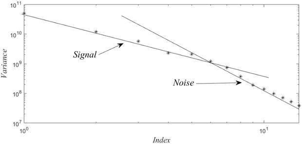
where $U={{}_{5716}U}^{15};V={{}_{5716}V}^{15}$, and $\mathrm{\Lambda }$ is the 15 × 15 diagonal matrix of singular values. Note that (4) is exact. (The 15 × 15 matrix $G_S^{†}{G}_S$ generates$\mathrm{\Lambda }$ and V, from which U follows by elementary considerations. The plot below is a log-log plot of the spectrum of variances (squares of singular values).)

One can reasonably conclude from Figure 1, that the analysis can be reduced to the six modes, ahead of the knee, or intersection. Henceforth, we consider the induced six-dimensional representation,

Figure 1.

Log-log plots of the variances reveal that these follow two different power laws, which by routine arguments can be associated with signal or noise.

$$G_S=U\mathrm{\Lambda }{V}_t,$$E5

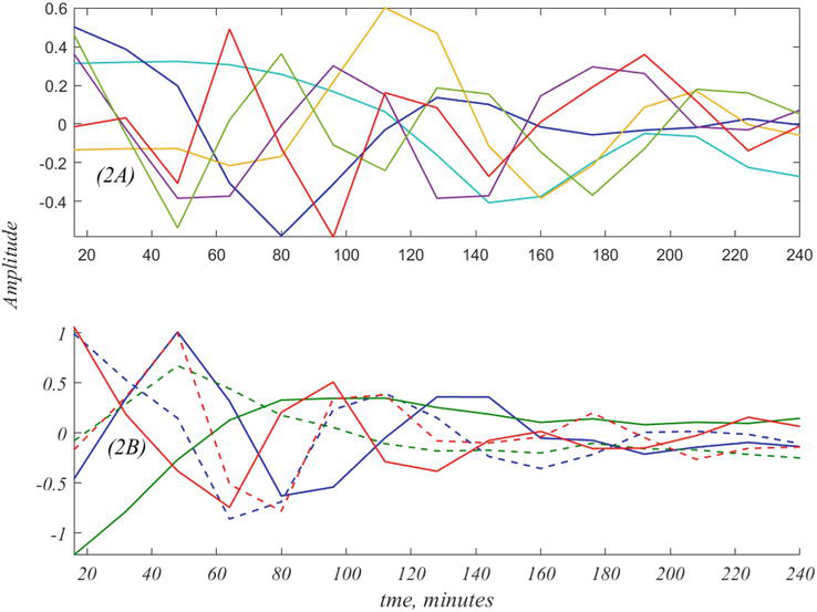
where V_t refer to the 6 × 15 time courses that result from SVD as plotted in Figure 2(A).

Figure 2.

The six time histories of V_t are shown in (A). The true underlying dynamics of the data is shown in (B), as obtained by dynamic mode decomposition, DMD [13], also see [14] and Section 8. This is composed of three complex modes, the real and imaginary parts of which, are depicted by the three colored pairs in (B). Further details are given below.

The plots of Figure 2(A) may be regarded as artifactual consequences of SVD, that only hint at the true dynamics. The goal of DMD is to recast the data in terms of the true exponential frequencies that are latent in the data. Thus, the curves of Figure 2(A) are entangled versions of the true dynamics, shown in Figure 2(B). In Section 8 we obtain the 6 × 6 matrix, E, that disentangles V_t, into the three complex modes shown in Figure 2(B). For the present, note that the decomposition

$$G_S=\left(U\mathrm{\Lambda }E\right)\left(E^{-1}{V}^{†}\right),$$E6

provides a generalization of SVD, (4), that is appropriate for data that have a rational dynamic ordering of columns.

3. High value genes

One can reasonably anticipate two limiting forms of gene expression; steady expression, as might be the case, for the proteins that form the cell wall and membrane; and a briefer activation and later inactivation on a shorter timescale, as might be the case for formation of the cell nucleus and its components. As a criterion for distinguishing these two limits consider the coefficient of variation,

$$C_V={\sigma }_G/\overline{G},$$E7

where ${\sigma }_G$ denotes the standard deviation of the time history of G, and $\overline{G}$, the mean value. For example, there are more than 1500 genes for which C_V < 0.1 and over 1100 for C_V > 0.25. In Table 1, the second line specifies six known CDC genes [6], with their coefficient of variation in the line above. Large C_V suggests that gene expression is due to transitory mechanisms, as will be explained below.

CV	0.1845	0.7216	0.3936	0.2337	0.6861	0.2903
Gene	YDL155W	YGR108W	YGR109C	YLR210W	YPR119W	YPR120C
CorrCoef	0.9843	0.9878	1	1	0.9950	0.9864
Gene	YMR144W	YGL021W	YGR109C	YLR210W	YGL021W	YJL181W
CV	0.3475	0.7222	0.3936	0.2337	0.7222	0.3128

Table 1.

Six known CDC genes [6], line 2. Their coefficients of variation, shown on line 1. Each are highly correlated, line 3, to the genes of line 4; each of which have the higher coefficients of variation, shown on line 5.

Co-regulation implies correlated activity. The fourth line of the table shows genes highly correlated to those of the second row, shown on the third line, to the genes of the second line. The implication of the Table is that the genes of the fourth line are better gene representatives. Peak times of two like genes are virtually identical.

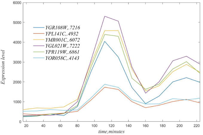
In general, any gene can be well correlated to many genes. This is illustrated in the next figure the for genes correlated with GR108W, with gene names and coefficients of variation in the legend. YGL021W with a C_V = 0.7222 the best exemplar of this set of highly correlated genes.

As is clear from Figure 3, peak locations, ipso facto, must occur at sampling locations, but would be better resolved by interpolation.

Figure 3.

Time courses of genes highly correlated to YGR108W, see legend. Note that each of these has a peak at t = 112, based on the experimental sampling.

3.1 Gene selection

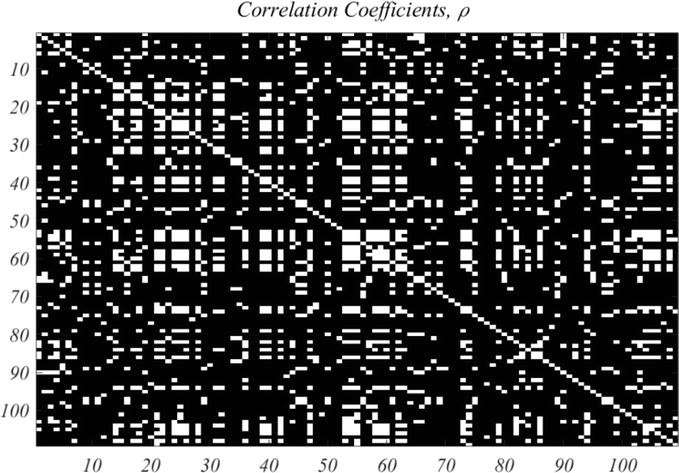
As mentioned above there are 1192 genes for which C_V > 0.25. These will be regarded as a starting point for selecting high value genes. A large number of traces exhibit pure exponential decay, starting at extremely high expression values, and are regarded as artefactual. Thus, a second criterion is restriction to time traces that start with relatively small expression, as is the case in Figure 3. For example, a restriction to initial value of a gene at 16 min, of <450, results in a well-correlated set of 109 genes. Figure 4 shows the correlation image based on the correlation criterion, $\rho >.85$ for the chosen set of 109 genes, in given order.

Figure 4.

Correlation coefficient of the 109 selected genes, with correlation coefficient, ρ, greater than .85 shown as white pixels.

The above figure is based on r = 6 and the 109 high-value genes. The SVD of the derived G_S for this case has the form,

$${G^{\ast }}_S=U^{\ast }{\mathrm{\Lambda }}^{\ast }{V_t}^{\ast },$$E8

where $U^{\ast }$ is 109 × 6, ${\mathrm{\Lambda }}^{\ast }=6\times 6$ and $V_t^{\ast }$ = 6 × 15. A straightforward calculation shows that this captures more than 99% of the variance of G_S. Figure 2 is also based on these choices.

4. Analysis of the high value genes

The DMD analysis of $G^{\ast }$ produces three complex modes with complex frequencies,

$$\left[{\mathrm{\Omega }}_1,{\mathrm{\Omega }}_2,{\mathrm{\Omega }}_3\right]\approx \left[‐.018\pm .032\mathrm{i};‐.022\pm 0.0906\mathrm{i};‐.013\pm .069\mathrm{i}\right].$$E9

${\mathrm{\Omega }}_3$ is identified with daughter cells, with period$T_3=2\pi /{\mathrm{\Omega }}_3\approx$ 92 min; ${\mathrm{\Omega }}_2$ is identified with mother cells, with period T₂$=2\pi /{\mathrm{\Omega }}_2\approx 71\mathit{min}$. (Smaller daughter cells are well known to take longer to mature.) Depending upon the complexion of the gene sets chosen, there is a range of values for these two periods, however the big picture remains the same. The first period, T₁, is roughly 200 min, close to the duration of the experiment. The time courses following from DMD, and take the form,

$$V_t\approx Eexp\left(\mathrm{\Omega }t\right)E^{-1}{V}_0,$$E10

where V_o is the initial value, and E is derived from the data, and t is given by (2). The exponential matrix in (10) is given by

$$exp\left(\mathrm{\Omega }t\right)=\left[\begin{array}{ccc}\exp \left({\mathrm{\Omega }}_{1}t\right)& 0& 0\\ 0& exp\left({\mathrm{\Omega }}_{2}t\right)& 0\\ 0& 0& exp\left({\mathrm{\Omega }}_{3}t\right)\end{array}\right].$$E11

This form speaks volumes. Since each $exp\left(\mathrm{\Omega }t\right)$ is a diagonal matrix, these entries are pure exponentials, and thus from (10)$E^{-1}{V}_t$ disentangles the modes into exponentials. Support for this assertion is shown in Figure 2. On this basis, for data sets of a dynamical type, SVD is generalized by

$$G-\overline{G}=G_S=\left(U\mathrm{\Lambda }E\right)\times \left(E^{-1}{V}_t\right)$$E12

where $\left(E^{-1}{V}_t\right)$, produces un-entangled temporal modes, with amplitudes, $\left(U\mathrm{\Lambda }E\right).$

And enduring puzzle of SVD analysis has been the origin of the time courses of V. This was solved by Schmid [13] with his discovery of DMD, as discussed above. This observation applies, generally, to data of dynamical type, and in particular for our data with the result,

$$G_s=\left(U\mathrm{\Lambda }E\right)\left(exp\left(\mathrm{\Omega }t\right)E^{-1}{V}_0.\right)$$E13

4.1 Unfolding the CDC

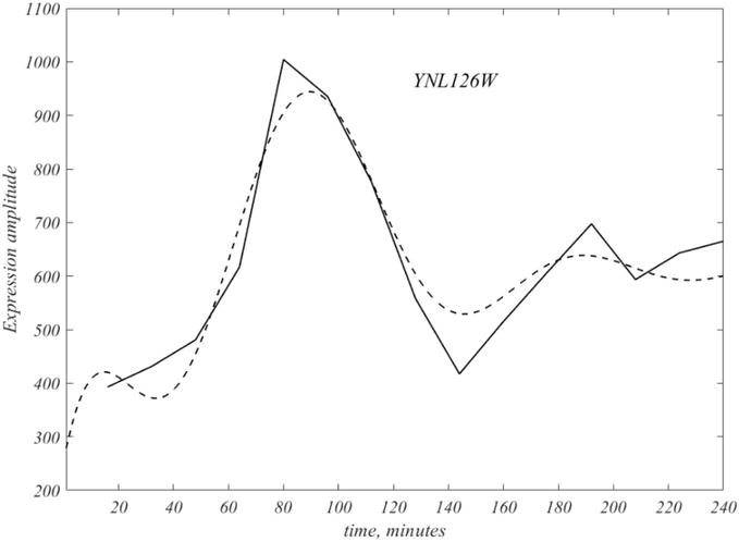
The goal is acquisition of a data-based model of the CDC, under the assumption that CDC is a temporal unfolding of genes, with defined activation times. As is clear from Figure 3, time resolution is limited by course sample times. The exponential representation of (13) induces a natural Fourier representation that overcomes this limitation. From the calculated frequencies, (9), we can sample every minute, including the first 16 min. In Figure 5, the smooth version of the indicated gene is shown as a dashed curve, and compared with the disentangled experimental modes, (12), in order to convey a sense of the Fourier form, as well as the improved peak locations.

Figure 5.

The dashed curve represents the Fourier interpolated version of the original polygonal data of the gene YNL126W, and is the first of the 109 genes. Note the interpolation covers the initial 16 min, and also runs over the second attenuated cycle.

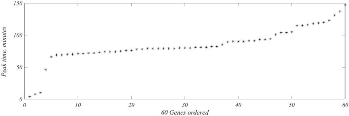
Inspection of the 109 highly sampled genes reveals that 43 take on negative values, and 8 have a peak at t = 1. Both conditions are regarded as unacceptable and the corresponding genes will be dropped from consideration. The result is a set of 60 genes that have peak expression times, $\left\{T_j\right\},$ shown in Figure 6.

Figure 6.

Times, $\left\{T_j\right\},$ of peak appearance, y-axis, of the 60 choice genes.

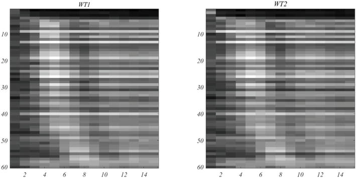
In Figure 7, the left image shows the trajectory of gene expression for peak times arranged in ascending order. This compares favorably with the phase plots that appear in [6]. At the right is the comparable plot for WT2 under the same gene ordering. It should be noted that the Orlando et al. plots are based on their 440 consensus genes. That set contains seven of the present high-value 60 genes, while the co-regulated set of 800 genes in [8], contain 42 of the 60 high-value genes. The table of 60 high-value genes, and their properties appear in the Supplement.

Figure 7.

Track of mRNA expression of the 60 selected genes, $G_{\mathit{ord}}^{60}$, arranged in ascending order of peak activation time. As in Orlando et al. [6], a log transformation has been applied to enhance the image.

5. Coherent gene sets

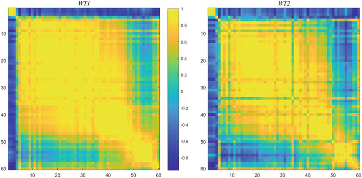
Here, co-regulated implies well-correlated, and we next construct the temporal correlation coefficients. For this purpose, the genes will be ordered as they unfold. This arrangement will be denoted by $G_{\mathit{ord}}^{60}$. The correlation coefficients of $G_{\mathit{ord}}^{60}$, are shown at the left of Figure 8.

Figure 8.

Correlation coefficients, ρ, of $G_{\mathit{ord}}^{60}$, as time ordered, for WT1 and WT2.

The figure on the right is the result of the same calculation, based on the selected ordering applied to WT2. This provides a compelling demonstration that the 60 choice genes are “strongly co-regulated”, in general. A much larger set, 413 genes, similarly constructed, produces an intersection of 204 genes with the Spellman co-regulated set of 800.

Unfolding times is regarded as a reasonable hypothesis for gene ordering; though other possibilities may be considered. For example, ordering the genes in terms of descending correlations, ρ, or equivalently increasing temporal distance of time histories. This leads to heat plots and dendrograms, none of which were deemed productive.

6. The single yeast cell

Figure 3, exhibits a typical gene time course, and displays single gene expression duration over many tens of minutes. However, the accepted estimate for the duration of gene transcription and translation is 1–2 min [15], and for convenience this value is taken to be 1 min in the calculations performed below. To explain what might appear to be an inconsistency, we review the data acquisition procedure, and as will be seen is due to the different maturation periods of mother and daughter cells, and randomness.

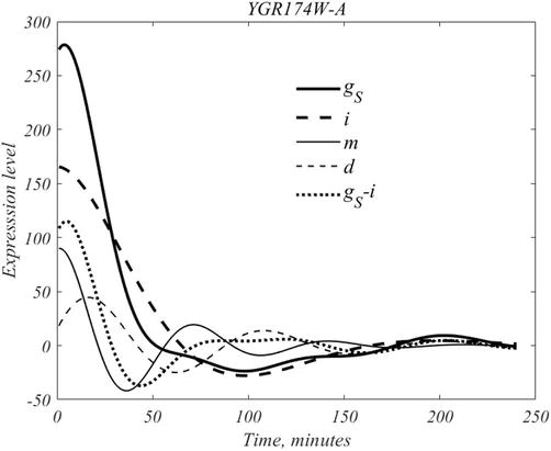
In experiments, after assembly of a suitable pool of yeast cells, aliquot removals along with genetic snapshots are obtained at 16 min intervals, and repeated 15 times. The result is the report of mRNA expression for each gene at each sampling instant. According to [6] each sampling, contains more than 200 yeast cells. To obtain a sense of the process consider gene YGR174-A, the earliest activated gene, of the 60 gene set, as deconstructed in Figure 9.

Figure 9.

The dynamical composition of gene YGR174W-A, the earliest activated gene. See text.

The mean subtracted form of this genes is denoted by g_S; DMD produces the four traces related by,

$$g_S-i=m+d,$$E14

where i, m, d represent the inherent, mother, daughter time courses.

The mother cohort, m, has a peak of 90 at t = 1, of period 71 min; and daughter cohort, d, a peak of 45 at 16 min and has period 92 min. The two entries in the left-hand side of (14) are defined over the full interval, and their difference has a peak of 115 at 5 min. If we denote by N_M and N_D the unknown number of mother and daughter cells that are participating in the signal, then straightforward back of the envelope calculation, based on peak quantities and locations, shows that N_M/N_D ∼ .285, from which the population fraction,

$$f=N_M/\left(N_D+N_M\right)\approx .22,$$E15

follows. Thus, there are more than three times as many daughter cells as mother cells in an average aliquot.

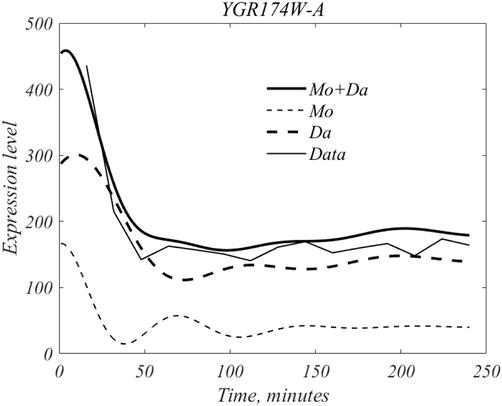
For formal purposes the inherent signal and the mean will be divided into 2 parts, as follows,

$$\begin{array}{l}\mathit{Mo}=m+f\times \left(i+g_m\right)\\ \mathit{Da}=d+\left(1-f\right)\times \left(i+g_m\right),\end{array}$$E16

so that the total signal is equals Mo + Da.

where mother, daughter, inherent and mean our shown in Figure 9. As shown in Figure 10, the full signal this gene equals Mo + Da.

Figure 10.

Mother cell dynamics are initiated at roughly t = 0, and daughter cell dynamics at roughly 10 min, with each being responsible for a steady production at large t. The two add to yield the overall gene activity shown in the heavy curve.

To summarize, genes are expressed both in a background manner, inherent expression, and in a scheduled manner, to peak at some specific time. It is also clear from this analysis that the activities of mother and daughter cells are not coupled.

6.1 A yeast model

Next, we consider a proposed computational model of the yeast cell. For this we focus on the gene traces displayed in Figure 10. While additional genes might be included in the model, the uncertainties in experimental results [15, 16] do not justify such generalizations. Our purpose in this exercise is merely to demonstrates that a practical framework can be created.

To start, it is noted that estimates of protein molecules per yeast cell are in the range of ∼$5\times {10}^7$ [15]. Since there are roughly 6000 genes in the yeast cell under consideration, the estimated number of such molecules per gene is ∼$5\times {10}^7/6000\approx 8.3\times {10}^3.$ This is a ballpark figure, and in this spirit other considerations such as protein degradation will be ignored. Further, the duration of proteins expression will be taken as 1 min. If we denote the mother and daughter dynamics of Figure 10 by $m\left(t\right)\&d\left(t\right)$, respectively, the number of proteins at maturation for mother and daughter cells is estimated from by,

$$\begin{array}{l}{p}_M=\sum _{i=1}^{71}\mathit{Mo}\left(t_i\right)\approx 4.53\times {10}^3,\\ p_D=\sum _{i=1}^{92}\mathit{Da}\left(t_i\right)\approx 1.75\times {10}^4.\end{array}$$E17

The ratio p_D/p_M = .26 is remarkably close to the above mentioned N_M/N_D ∼ .285. Since these estimates are in the range of the ballpark gene estimate of $8.3\times {10}^3$, it is surmised that the Orlando et al. [6] data was normalized by the estimated number of cells in an aliquots, >200. These considerations also suggest that cell size differences of mother and daughter cells plays little or no role in protein content at maturation.

On the basis of these deliberations one might contemplate creating an algorithmic model of the CDC. Randomization can be introduced through variations in mother and daughter CDC periods, and variations in the number of mother and daughter cells, say adding up to roughly 200. This is a future project, which can useful only with better knowledge and precision of the quantities involved.

7. Additional comments

The high degree of correlation, seen in Figure 6 tells little beyond timing. For example, it does not imply anything certain about gene interactions, nor is there any information about the activation and deactivation times of genes. The mechanism by which budding yeast cell assembles itself, is an open question. Since no outside intervention is in play, it is noncontroversial to presume, that the cell self-assembles. Just how this self-assembly takes place is another open question, it might e.g. only be a matter of proteins falling into their proper place, based on the timing of gene expression. In this case the cell model is an assembly line for proteins that arrive in an orderly fashion.

In an effort to introduce some additional theory it is noted activation and inactivation of gene expression may be likened to an equilibrium disturbance, followed by restoration, (suggestive of wave phenomena.). In this connection it is noted that the mother and daughter modes that describe the CDC each follow oscillator dynamics [9]

$$\frac{d^{2}g}{{\mathit{dt}}^2}+2\lambda \frac{\mathit{dg}}{\mathit{dt}}+\left({\lambda }^2+{\omega }^2\right)g=0,$$E18

which has solutions in the form,

$$g\propto exp\left[\left(-\lambda \pm \mathit{i\omega }\right)t\right].$$E19

In this connection, we can define a new variable, v, by,

$$\frac{\partial g}{\partial t}=\frac{\omega }{2\pi }v,$$E20

which since $2\pi /\omega$ gives the period of mRNA, might be reasonably associated with rate of protein production, and from (18)v is governed by

$$\frac{\partial v}{\partial t}+2\mathit{\lambda v}+\left({\lambda }^2+{\omega }^2\right)\frac{2\mathit{\pi g}}{\omega }=0.$$E21

The pair of Eqs. (20) and (21) may be viewed as a coarse-grained version of the central dogma.mentioned the dynamics of transcription and translation occurs on a scale of ∼1 min, or so. As dictated by the experiments, our deliberations are based on timescales large compared to 1 min, and thus, only genes and their proteins can figure in the description. This is consistent with “one gene-one polypeptide” view of [17]. Impressionistically, this Beadle-Tatum view is a macroscopic description.

A key result of the present investigation is the remarkable ability of DMD, to distinguish dynamic characteristics of the mother and daughter cohorts. Gene experiments typically attempt to sequester daughter cohorts, and it is natural on the basis of the methods pursued here to consider what the outcome would have been of considering complementary populations, and furthermore to monitor the base population, without any form of sequestering. Given the remarkable ability of DMD to parse dynamic activity more complicated population yeast populations might be considered. Hopefully, this ability to distinguish yeast subpopulations will lead to new ways to probe into the yeast life form. Another future goal, is that the algorithmic model touched on here can be further advanced, since a falsifiable model is always desirable.

8. Methods

8.1 Dynamic mode decomposition

Traditional signal analysis is based on the hypothesis that a signal is an admixture of sinusoids, and therefore that Fourier analysis can decompose the signal into his Fourier components. DMD may be regarded as an extension of this idea. Suppose for real λ & ω, we define a complex frequency,

$$z=\lambda +\mathit{i\omega },$$E22

with corresponding complex signal,

$$s\sim \alpha exp\left(\mathit{zt}\right)=\alpha exp\left(\mathit{\lambda t}\right)\cdot \left[cos\mathit{\omega t}+isin\mathit{\omega t}\right].$$E23

DMD can be regarded as a method for extracting such a signal, and more generally, admixtures of such signals. In this respect Fourier analysis is a subset of DMD.

Typically, a laboratory signal is a uniformly sampled version of the continuous case. Suppose for example the uniformly sampled times are,

$$t=\left[\mathit{dt},2\mathit{dt},\cdots ,\mathit{Ndt}\right];$$E24

in which case (23) becomes the geometric sequence.

$$S=\left[s_1,\dots ,s_N\right]=\left[{\delta }^1,\dots ,{\delta }^N\right]\alpha$$E25

where

$$\delta =exp\left(\lambda \cdot \mathit{dt}\right),$$E26

which is therefore the generator of the sampled signal. Reciprocally, if $\left\{s_j\right\}$ is (noisy) data, we can seek a generator, A, such that

$$s_{j+1}={\mathit{As}}_j,j=1,\dots ,N-1,$$E27

which can be viewed as a case of many equations for the one unknown, A. Least squares is the suggested approach in this case. The error in applying (27) is

$$\mathit{Er}=\sum _{k=1}^{N-1}{‖s_{k+1}-{\mathit{As}}_k‖}^2,$$E28

and the (least-squares) minimization of (28) produces the solution

$$A=\sum _{k=1}^{N-1}{s}_{k+1}{\theta }_k;{\theta }_k=s_k/\sum _{k=1}^{N-1}{s}_k^2.$$E29

A more compact form is obtained by defining the vectors,

$$S1=\left[s_1,\dots ,s_{N-1}\right]\&S2=\left[s_2,\dots ,s_N\right]$$E30

in which terms (29) can be written as

$$\theta =S1/{‖S1‖}^2.A=\left(S2,\theta \right).$$E31

for later purposes observe that if the problem is posed as,

$$A\times S1=S2,$$E32

then it is solved by

$$A=S2\times S{1}^{+},$$E33

where $S{1}^{+}$ is referred to as the Moore-Penrose inverse [18]. Clearly, $S{1}^{+}=\theta ,$ and (33) is equivalent to minimizing (28). Briefly stated, the Moore Penrose inverse has the smallest norm of the many solutions that solve (32).

In the general case, of multiple complex signals, we are confronted by a matrix V(t),

$$V_{\mathit{ij}},i=1,\dots ,M;j=1,\dots ,N,$$E34

with M time histories, each sampled uniformly N times. For example $V_t^{\ast }$(8) is 6 × 15. Under the hypothesis that the data is composed of complex exponentials, one can seek the generator matrix, A by defining

$$\begin{array}{l}V1=V\left(i,1\le j\le N-1\right)\\ V2=V\left(i,2\le j\le N\right)\end{array}$$E35

so that

$$\mathit{AV}1=V2$$E36

which is solved by the Moore-Penrose inverse, $V{1}^{+}$.

$$A=V2\times V{1}^{+}.$$E37

The spectral decomposition of the generator matrix, A,

$$A=E\mathrm{\Sigma }\left(t\right)E^{-1},$$E38

produce complex frequencies as eigenvalues of the diagonal matrix $\mathrm{\Sigma }$, and that the corresponding eigenvectors in E disentangle the time courses produced by SVD. Evidence supporting both assertions appear in the data analysis. The construction (38) permits generalization of SVD, (6). If we write

$$\mathrm{\Sigma }\left(t\right)=\left(\begin{array}{ccc}{\sigma }_1\left(t\right)& 0& 0\\ 0& \ddots & 0\\ 0& 0& {\sigma }_n\left(t\right)\end{array}\right),$$E39

where n = 6 in the yeast application, then it proves to be convenient to transform to the hypothesized exponential form

$$\mathrm{\Omega }=-log\sigma /\mathit{dt},$$E40

which is just the inverse of (26). dt is the sampling interval (2) and (39) transforms to (11).

In the interest of brevity, we forgo examples. Consideration of synthetic data generated by,

$$D\left(\mathrm{\Omega },M\right)=\sum _{j=1}^{m}exp\left({\lambda }_{j}t\right)\left({\alpha }_{\mathit{ij}}cos\left({\omega }_{j}t\right)+{\beta }_{\mathit{ij}}sin\left({\omega }_{j}t\right)\right);i=1,2\dots ,M,$$E41

with each of the M trials an admixture of m complex signals and randomly chosen coefficients shows a remarkable accuracy in recovering the frequency content after relatively few trials.

9. Conclusions

This paper represents a substantial extension of an earlier preliminary analysis [9] of the high quality yeast database assembled by Orlando et al. [6].

The principal focus of this paper is the introduction of advanced mathematical methods that should be useful under a wider set of circumstances. For example, for general dynamical molecular biological data sets, and for when better resolved data becomes available for S. cerevisiae studies. Since the Orlando data is sampled at a large fraction of the CDC cycle, and near the Nyquist limit [19], the data is broadly speaking, and out of necessity, under-sampled. For this reason and for purposes of exposition the Orlando data has been converted to interpolated version, by Fourier methods to get a grip on what might potentially t be achieved with better sampled data, see Figure 5. This leads to a description of the CDC in terms of precise times of gene activation and deactivation, which are likely only a semblance of the true times. Another focus has been on the concept of co-regulation, as introduced by Spellman et al. [8], which in the present analysis is reformulated as obtaining gene collections that are highly correlated with one another. Within this very approximate framework a set of roughly 100 genes is proposed as being central to the CDC, and which again is only a semblance of what truly are the co-regulated genes.

The Singular Value Decomposition, SVD, is the chosen mathematical framework for dealing with the dynamical structure of the yeast data and is believed likely to play an important role in examining dynamical biological data of a general nature. A shortcoming of SVD is that the dynamics generated by SVD is severely constrained by the underlying methodology of SVD. This shortcoming was repaired by Schmidt [13], by a method that is termed dynamic mode decomposition, DMD. This is fully treated in Section 8 of this paper, in particular see (13). In brief, the result is that the CDC is well approximated by a single mode that depicts the dynamics in terms of timescales representative of mother cells, and daughter cells.

It is an opinion that future more highly sampled data lead to the same qualitative description that is more refined, and accurate.

References

1.Watson JD, Crick FH. Molecular structure of nucleic acids: A structure for deoxyribose nucleic acid. Nature. (Wiley, New York). 1953;171(4356):737-738
2.Neumann JV. The General and Logical Theory of Automata. Vol. 1951. New York: Wiley; 1951. pp. 1-41
3.Schrödinger E. What is Life?: With Mind and Matter and Autobiographical Sketches. Cambridge University Press; 1992
4.Nirenberg MW, Matthaei JH. The dependence of cell-free protein synthesis in E. coli upon naturally occurring or synthetic polyribonucleotides. Proceedings of the National Academy of Sciences. 1961;47(10):1588-1602
5.Crick F. Central dogma of molecular biology. Nature. 1970;227(5258):561-563
6.Orlando DA et al. Global control of cell-cycle transcription by coupled CDK and network oscillators. Nature. 2008;453(7197):944-947
7.Cho RJ et al. A genome-wide transcriptional analysis of the mitotic cell cycle. Molecular Cell. 1998;2(1):65-73
8.Spellman PT et al. Comprehensive identification of cell cycle–regulated genes of the yeast Saccharomyces cerevisiae by microarray hybridization. Molecular Biology of the Cell. 1998;9(12):3273-3297
9.Sirovich L. A novel analysis of gene array data: Yeast cell cycle. Biology Methods and Protocols. 2020;5(1)1-10
10.Tyson JJ. Modeling the cell division cycle: cdc2 and cyclin interactions. Proceedings of the National Academy of Sciences. 1991;88(16):7328-7332
11.Sirovich L. Turbulence and the dynamics of coherent structures. I. Coherent structures. Quarterly of Applied Mathematics. 1987;45(3):561-571
12.Lax PD. Linear Algebra and its Applications. New York: Wiley; 2007. p. 2007
13.Schmid PJ. Dynamic mode decomposition of numerical and experimental data. Journal of Fluid Mechanics. 2010;656:5-28
14.Kutz JN et al. Dynamic Mode Decomposition: Data-Driven Modeling of Complex Systems. Philadelphia: SIAM; 2016
15.Milo R, Phillips R. Cell Biology by the Numbers. New York: Garland Science; 2015
16.Gerstein MB et al. What is a gene, post-ENCODE? History and updated definition. Genome Research. 2007;17(6):669-681
17.Beadle GW, Tatum EL. Genetic control of biochemical reactions in Neurospora. Proceedings of the National Academy of Sciences of the United States of America. 1941;27(11):499
18.Golub GH, Van Loan CF. Matrix Computation. 1989. Johns Hopkins. Baltimore, MD: University Press; 1989
19.Nyquist H. Certain topics in telegraph transmission theory. Transactions of the American Institute of Electrical Engineers. 1928;47(2):617-644
Written By
Lawrence Sirovich
Submitted: 06 October 2023Reviewed: 18 October 2023Published: 27 November 2023
Open access peer-reviewed chapter