Method for GPS-Monitoring of Small-Scale Fluctuations of the Total Electron Content of the Ionosphere for Predicting the Noise Immunity of Satellite Communications

Abstract

The chapter is devoted to the development of a method for monitoring small-scale fluctuations in the total electronic content of the ionosphere using signals from global navigation satellite systems GPS/GLONASS and for evaluating the characteristics of such fluctuations in the interests of analyzing the noise immunity of satellite communication systems. The proposed method is based on digital processing of measurement results obtained using the advanced capabilities of the NovAtel GPStation-6 receiver and allows to estimate the root mean square of small-scale fluctuations in the total electron content of the ionosphere, the ionospheric scintillation index and to predict the changes in the noise immunity of satellite communication systems.

1. Introduction

It is known [1, 2, 3, 4, 5, 6, 7, 8, 9] that the propagation of radio waves in satellite systems under conditions of the formation of intense small-scale irregularities in the Earth’s ionosphere is accompanied by the appearance of ionospheric scintillation (fading) of received signals. These effects can lead to a significant decrease in the noise immunity of satellite communication systems (SCS) because of the occurrence of errors when receiving messages. Therefore it is necessary to monitor small-scale irregularities of the ionosphere and to predict changes in the noise immunity of SCS during ionospheric disturbances.

To measure the characteristics of large-scale irregularities of the ionosphere, GPS monitoring methods are most widely used. GPS monitoring is based on measuring the total electron content (TEC) in a radio line of global navigation satellite systems (GNSS) using a dual-frequency receiver. However, ionospheric scintillation is generated not by large-scale fluctuations of the ionospheric TEC, but by its small-scale fluctuations, which are not currently measured by a dual-frequency GNSS receiver. Therefore, the task of modifying a dual-frequency GNSS receiver in the direction of separating (filtering) small-scale TEC fluctuations from fluctuations of larger scales and subsequent determination of their statistical characteristics is very actual.

The aim of the work is to develop a method for GPS monitoring of small-scale fluctuations of ionospheric TEC and their use for predicting changes in the noise immunity of SCS during ionospheric disturbances.

2. Analysis of the effect of small-scale ionospheric irregularities on the noise immunity of satellite communication system

It is known [2, 3, 4, 5, 8, 9, 10, 11, 12] that the Earth’s ionosphere is constantly exposed to natural (solar activity, hurricanes, earthquakes, etc.) disturbing factors that cause change in its electron concentration $N\left(h,\rho \right)$ (${\mathrm{m}}^{-3}$) in height ($h$) and space ($\rho =x,y$). This change manifests itself in the formation of vast (up to several hundred and thousands of kilometers) regions (Figure 1), in which the electron concentration $N\left(\rho ,h\right)=\overline{N}\left(h\right)+\mathrm{\Delta }N\left(\rho ,h\right)$ differs from the average value $\overline{N}\left(h\right)$ due to the formation of irregularities $\mathrm{\Delta }N\left(\rho ,h\right)$ of various spatial scales (from hundreds of kilometers to tens of meters).

Figure 1.

A model of the ionosphere with small-scale irregularities (a) and trans-ionospheric radio wave propagation (b).

The cause of ionospheric scintillation is small-scale irregularities of electron concentration $\mathrm{\Delta }N\left(\rho ,h\right)$, which are characterized by sizes $l_s\approx \mathrm{10...1000}\mathrm{m}$. The magnitude of relative fluctuations ($\mathrm{\Delta }N/\overline{N}$) of the electron concentration in small-scale irregularities at any height ($h$) is practically constant [2, 5, 6, 10]: $\mathrm{\Delta }N/\overline{N}\approx \mathrm{\Delta }N\left(\rho ,h\right)/\overline{N}\left(h\right)\approx {10}^{-3}$. Therefore, the greatest fluctuations of the electron concentration will be observed (Figure 1) at the heights of the maximum ionized layer F ($h_{\max }\approx \mathrm{250...350}\mathrm{km}$) of the ionosphere: $\mathrm{\Delta }N\left(\rho ,h_{\max }\right)\approx {10}^{-3}\overline{N}\left(h_{\max }\right)$. With natural and artificial disturbances of the ionosphere, these fluctuations can increase by 1–2 orders of magnitude [2, 3, 4, 8, 10] up to $\mathrm{\Delta }N\left(\rho ,h_{\max }\right)\approx \left({10}^{-2}{\mathrm{...10}}^{-1}\right)\overline{N}\left(h_{\max }\right)$. This makes it possible to represent a set of small-scale irregularities of the ionosphere on the path of propagation of radio waves from the satellite to the receiver in the form of a thin layer (phase screen), which is described by spatial small-scale TEC fluctuations [2, 8]

$$\mathrm{\Delta }{N}_T\left(\rho \right)=\underset{0}{\overset{\infty }{\int }}\mathrm{\Delta }N\left(\rho ,h\right)\mathit{dh}$$E1

relative to its average value ${\overline{N}}_T=\underset{0}{\overset{\infty }{\int }}\overline{N}\left(h\right)\mathit{dh}$ (${\mathrm{m}}^{-2}$). According to Eq. (1), with ionospheric disturbances, small-scale TEC fluctuations can increase by 1–2 orders of magnitude.

According to [2, 7, 8], the process of radio wave propagation (Figure 1) with a carrier frequency $f_0$ from the SCS satellite to the receiver through an ionospheric layer with small-scale irregularities (phase screen) is accompanied by distortions (fluctuations) of its phase front within the region of space $\rho$ bounded by the diameter of the first Fresnel zone ($l_F\approx 2\sqrt{{\mathit{ch}}_{\max }/f_0}\ge l_s$):

$$\mathrm{\Delta }\phi \left(\rho \right)=-80,8\pi \mathrm{\Delta }{N}_T\left(\rho \right)/{\mathit{сf}}_0,\mathrm{rad},$$E2

where $с$ – the speed of light ($\mathrm{m}/\mathrm{s}$); 80,8 – coefficient having dimension ${\mathrm{m}}^3/{\mathrm{s}}^2$.

The interference of individual sections ($\rho$) of the phase front of the wave Eq. (2) behind the phase screen causes a redistribution of the amplitude $A\left(\rho ,h\right)$ along the wave front (illustrated in Figure 1 in the form of a change in its thickness). These diffraction processes determine the instantaneous value of the signal power $P_r=A^2$ at the receiver input. Therefore, a change in the spatial TEC fluctuations $\mathrm{\Delta }{N}_T\left(\rho \right)$ along the wave propagation path due to the drift of small-scale irregularities and the motion of the satellite leads to a random change in the power of received signal carrier ($P_r$)—fading or scintillation. It leads to change in the ratio $P_r/N_0\equiv C/N_0$ of signal power to the spectral power density of noise ($N_0$) at the receiver input (carrier-to-noise ratio). To assess the degree of manifestation of this scintillation, the value of the scintillation index is traditionally used [1, 2, 3, 4, 9, 13]

$$S_4=\sqrt{\left(⟨P_r^2⟩-{⟨P_r⟩}^2\right)/{⟨P_r⟩}^2},$$E3

where $⟨x⟩$—designation of statistical averaging of random values $x$.

As an illustration, Figure 2 shows the changes in the carrier-to-noise ratio ($C/N_0$) and the scintillation index ($S_4$) of the GNSS GLONASS signal in the L1 frequency range obtained using the NovAtel GPStation-6 receiver, which is located at the North-Caucasus Federal University (Stavropol, Russia).

Figure 2.

Changes in the carrier-to-noise ratio (top panel) and the scintillation index (bottom panel) of the GNSS GLONASS signal in the L1 frequency range.

Analysis of Figure 2 shows that ionospheric scintillation is manifested around 12:56:40 local time (UTC + 3) by a sharp decrease in the carrier-to-noise ratio by 2…3 dB for about 20 seconds. This leads to a short-term increase in the scintillation index by almost 2 times (from $S_4\approx 0.1$ to $S_4\approx 0.17$). According to [1, 2, 3, 4, 8, 9, 14] in natural conditions, such short-term scintillation with relatively low intensity ($S_4=\mathrm{0.01...0.15}$) is characteristic of mid-latitude regions. In the polar regions, the scintillation is more intense ($S_4=\mathrm{0.45...0.7}$) and lasts from a few seconds to several minutes. In the equatorial regions, scintillation can last from several minutes to several hours and the scintillation index can reach $S_4=\mathrm{0.9...1}$. It is obvious that such significant differences in the intensity and duration of scintillation depend on the degree of local changes in the ionosphere electron concentration and the causes of their occurrence.

In the absence of small-scale fluctuations of the ionosphere electron concentration and TEC ($\mathrm{\Delta }{N}_T\left(\rho \right)\sim \mathrm{\Delta }N\left(\rho ,h\right)\to 0$) phase fluctuations in the wave front at the output of the ionosphere Eq. (2) will be absent ($\mathrm{\Delta }\phi \left(\rho \right)\sim \mathrm{\Delta }{N}_T\left(\rho \right)\to 0$). It causes the absence of diffraction effects and scintillation of the received signals ($S_4\to 0$). As the small-scale TEC fluctuations ($\mathrm{\Delta }{N}_T\left(\rho \right)$) increase or carrier frequency ($f_0$) decrease, the phase fluctuations in the wave front $\mathrm{\Delta }\phi \left(\rho \right)\sim \mathrm{\Delta }{N}_T\left(\rho \right)/f_0$ will increase proportionally. It follows that the ionospheric scintillation index ($S_4\sim {\sigma }_{\phi }$) will increase with increasing root mean square (RMS) ${\sigma }_{\phi }={⟨\mathrm{\Delta }{\phi }^2\left(\rho \right)⟩}^{1/2}$ of the phase front fluctuations at the ionospheric output (phase screen).

For the case when the fluctuations of the phase front $\mathrm{\Delta }\phi \left(\rho \right)$ at the output of the phase screen are described by a Gaussian probability distribution with zero mathematical expectation and dispersion ${\sigma }_{\phi }^2$, the dependence $S_4=\psi \left({\sigma }_{\phi }\right)$ has the form [13]

$$S_4=\sqrt{1-exp\left(-2{\sigma }_{\phi }^2\right)}.$$E4

Taking into account Eq. (2) the RMS of the fluctuations of the phase front at the ionosphere output (${\sigma }_{\phi }$) is determined by the RMS of small-scale TEC fluctuations ${\sigma }_{\mathrm{\Delta }{N}_T}={⟨\mathrm{\Delta }{N}_T^2\left(\rho \right)⟩}^{1/2}$ and the carrier frequency $f_0$ [2, 8]:

$${\sigma }_{\phi }=80,8{\mathit{\pi \sigma }}_{\mathrm{\Delta }{N}_T}/{\mathit{сf}}_0.$$E5

Thus, in accordance with Eqs. (4) and (5), the following dependence $S_4=\psi \left({\sigma }_{\mathrm{\Delta }{N}_T}\right)$ of the ionospheric scintillation index on the small-scale TEC fluctuations takes place [9]:

$$S_4=\sqrt{1-exp\left(-2{\left(80,8{\mathit{\pi \sigma }}_{\mathrm{\Delta }{N}_T}/{\mathit{сf}}_0\right)}^2\right)}.$$E6

The analysis showed that, in accordance with Eqs. (3)–(6), as the small-scale TEC fluctuations (${\sigma }_{\mathrm{\Delta }{N}_T}$) and the phase front fluctuations of the output wave (${\sigma }_{\phi }\sim {\sigma }_{\mathrm{\Delta }{N}_T}/f_0$) increase, the ionospheric scintillation index ($S_4\sim {\sigma }_{\phi }\sim {\sigma }_{\mathrm{\Delta }{N}_T}/f_0$) increases. Under these conditions, the quality of SCS functioning can significantly decrease due to the occurrence of errors when receiving messages. Signals with offset binary phase shift keying (OBPSK) are most commonly used to transmit messages in SCS. The probability of error ($P_{\mathit{err}}$) when receiving such signals with a constant average signal-to-noise energy ratio at the receiver input ($⟨h^2⟩$) under conditions of ionospheric scintillation (characterized by Nakagami distribution) is determined by the expression [15]:

$$P_{\mathit{err}}=\frac{1}{2}{\left(\frac{m}{m+⟨h^2⟩}\right)}^m=\frac{1}{2}{\left(\frac{{S_4}^{-2}}{{S_4}^{-2}+⟨h^2⟩}\right)}^{{S_4}^{-2}},$$E7

where $m=1/S_4^2$—Nakagami distribution parameter.

The analysis of Eq. (7) taking into account Eqs. (3)–(6) allows us to conclude that as the small-scale TEC fluctuations (${\sigma }_{\mathrm{\Delta }{N}_T}$) increase, the ionospheric scintillation index ($S_4\sim {\sigma }_{\mathrm{\Delta }{N}_T}/f_0$) and the probability of error ($P_{\mathit{err}}\sim 1/m\sim S_4$) when receiving signals that correspond to the elementary symbols of the transmitted message increase. Therefore, the prediction of its changes during ionospheric disturbances is an actual problem.

It is possible to solve this problem in two ways based on the results of monitoring the scintillation index ($S_4$):

1. in accordance with Eqs. (3) and (7) based on the results of measuring fluctuations of the received signal power ($P_r$) in GNSS;

2. in accordance with Eqs. (6) and (7) based on the results of the measurement of small-scale TEC fluctuations (${\sigma }_{\mathrm{\Delta }{N}_T}$).

Evaluation of the scintillation index $S_4$ is currently carried out using specialized dual-frequency GNSS receivers of the GISTM class (GNSS Ionospheric Scintillation and TEC Monitor) [11, 16, 17]. However, it is impractical to use them (including GPStation-6) to estimate the ionospheric scintillation index in the interests of noise immunity prediction for three reasons.

Firstly, the calculation of the scintillation index ($S_4$) in these receivers is carried out according to Eq. (3) based on the measurement of fluctuations of the received signal power ($P_r$). At low elevation angles of the GNSS satellite ($\alpha <5°\mathrm{...15}°$), scintillation can be caused not only by small-scale ionospheric irregularities but also by multiple reflection of radio waves from a variety of objects surrounding the receiving antenna. Therefore, the reliability of the calculation of the scintillation index, in this case, will be lower than on the basis of the estimation of small-scale fluctuations of the ionospheric TEC (Eq. (6)).

Secondly, the sampling interval of the results of calculating the scintillation index ($S_4$) in modern receivers usually does not exceed 1 minute. This means that its current value does not allow detection of short-term (lasting up to several seconds) occurrence of scintillation and reliably assess their intensity. This is confirmed by Figure 2.

Thirdly, the carrier frequency ($f_0$) in SCS may differ significantly from the carrier frequency of GNSS, so the scintillation indices ($S_4\sim {\sigma }_{\mathrm{\Delta }{N}_T}/f_0$) in different systems will also differ.

On the other hand, it is not possible to carry out an assessment of the RMS of small-scale fluctuations (${\sigma }_{\mathrm{\Delta }{N}_T}={⟨\mathrm{\Delta }{N}_T^2\left(\rho \right)⟩}^{1/2}$) based on the results of measuring the ionospheric TEC ($N_T$) using the GPStation-6 receiver for a number of reasons related to the complexity of separating (filtering) of small-scale TEC fluctuations ($\mathrm{\Delta }{N}_T$) with dimensions $\rho \approx l_s=\mathrm{10...1000}\mathrm{m}$ from large- and medium-scale TEC fluctuations with dimensions $\rho >l_s=1000\mathrm{m}$.

Therefore, the aim of the work is to develop a method for GPS monitoring of small-scale fluctuations of ionospheric TEC ($\mathrm{\Delta }{N}_T$) and their use for predicting changes in the noise immunity of SCS ($P_{\mathit{err}}\sim S_4\sim {\sigma }_{\mathrm{\Delta }{N}_T}/f_0$) during ionospheric disturbances. To achieve it first of all it is necessary to modify the GISTM-receiver for measuring small-scale TEC fluctuations ($\mathrm{\Delta }{N}_T$). Further, on this basis, it is possible to obtain estimates of the RMS of small-scale TEC fluctuations (${\sigma }_{\mathrm{\Delta }{N}_T}$), the ionospheric scintillation index in the SCS ($S_4\sim {\sigma }_{\mathrm{\Delta }{N}_T}/f_0$) according to Eq. (6) and to predict the changes in the noise immunity of the SCS ($P_{\mathit{err}}=\psi \left(S_4,⟨h^2⟩\right)$) according to Eq. (7).

3. Modification of the GPStation-6 receiver for measuring small-scale fluctuations of the total electron content of the ionosphere

It is known [11] that the method of GPS monitoring of the ionosphere based on the transmission of signals from the GNSS satellite at two carrier frequencies ($f_1$ and $f_2$) and the use of dual-frequency GNSS receivers allows to measure the values of the parameters of the received signals with high accuracy and on their basis to calculate not only the scintillation index ($S_4$) but also the ionospheric TEC ($N_T$).

Figure 3 shows a simplified structure for the construction of a dual-frequency receiver GPStation-6 for code measurements of ionospheric TEC (${\mathit{TEC}}_c$) and its modification for the evaluation of small-scale TEC fluctuations ($\mathrm{\Delta }{N}_T$). The receiver GPStation-6 consists of 2 main parts [17, 18]:

1. the hardware part includes a signal reception unit that performs analog-to-digital conversion, decoding of GNSS signals, and measurement of their main parameters: pseudo-ranges ($R_1^{\prime }$, $R_2^{\prime }$) to satellite and pseudo-phases (${\phi }_1^{\prime }$, ${\phi }_2^{\prime }$);

2. the software part implementing a digital processing unit in which the calculation of radio navigation parameters, receiver coordinates, scintillation index ($S_4$), ionospheric TEC (${\mathit{TEC}}_c$), etc., is carried out.

Figure 3.

The structure of the construction of the GPStation-6 dual-frequency receiver for code measurements of ionospheric TEC (${\mathit{TEC}}_c$) and its modification for the evaluation of small-scale TEC fluctuations ($\mathrm{\Delta }{N}_T$).

In order to estimate small-scale fluctuations of the ionospheric TEC ($\mathrm{\Delta }{N}_T$) based on the results of measuring the ionospheric TEC ($N_T$) using a dual-frequency receiver GPStation-6, it is necessary to modify its software (Figure 3).

The need for such a modification of the GPStation-6 receiver software is due to the following reasons. The principle of operation of the GISTM receiver is based on the results of measurements of the pseudo-range $R_i^{\prime }\sim R+40,4N_T/f_i^2$ to each of the navigation satellite (otherwise, code measurements). In addition to the true range $R$, they contain an ionospheric component that depends on the ionospheric TEC ($N_T$) on the route from the satellite to the receiver and the carrier frequency ($f_i$) [11, 16, 17]. Since the transmission of navigation signals in the GNSS is carried out simultaneously at two carrier frequencies ($f_1\approx 1,6\mathrm{GHz}$ and $f_2\approx 1,2\mathrm{GHz}$), it is possible to calculate the ionospheric TEC at each moment of time based on a linear combination (difference) of the measured pseudo-ranges ($R_1^{\prime }\sim R+N_T/f_1^2$ and $R_2^{\prime }\sim R+N_T/f_2^2$) [11, 19]:

$$\begin{array}{c}{\mathit{TEC}}_c=\frac{1}{40,4}\left(\frac{f_1^2{f}_2^2}{f_1^2-f_2^2}\right)\left(R_2^{\prime }-R_1^{\prime }\right)\\ =\frac{1}{40,4}\left(\frac{f_1^2{f}_2^2}{f_1^2-f_2^2}\right)\left(R_2-R_1\right)+{\delta }_d+{\delta }_n=N_T+{\delta }_d+{\delta }_n.\end{array}$$E8

According to Eq. (8), the results of the code measurements of the ionospheric TEC (${\mathit{TEC}}_c$) differ from its true value ($N_T$) by the amount of systematic error ${\delta }_d$ due to differential signal delays in transmitting and receiving radio paths, and random error ${\delta }_n$ due to the influence of internal receiver noise.

Code measurements of the TEC (${\mathit{TEC}}_c$) are made in the GPStation-6 receiver with a sampling interval ${\tau }_d=1\mathrm{s}$. Therefore, as discrete values accumulate, a time series is formed

$${\mathit{TEC}}_c\left(t\right)=N_T\left(t\right)+{\delta }_d+{\delta }_n.$$E9

In the general case of slant propagation of radio waves (at an angle $\alpha$ relative to the horizontal) through the ionosphere with electron concentration irregularities $N\left(\rho ,h\right)=\overline{N}\left(h\right)+\mathrm{\Delta }N\left(\rho ,h\right)$, the measured TEC, taking into account Eq. (1), is described as the sum of the regular (average) and fluctuation components:

$$N_T\left(\rho \right)=\underset{0}{\overset{\infty }{\int }}N\left(\rho ,h\right)\mathit{dz}=\underset{0}{\overset{\infty }{\int }}\overline{N}\left(h\right)\mathit{dz}+\underset{0}{\overset{\infty }{\int }}\mathrm{\Delta }N\left(\rho ,h\right)\mathit{dz}={\overline{N}}_T+\mathrm{\Delta }{N}_T\left(\rho \right),$$E10

where $\mathit{dz}\approx \mathit{dh}cosec\alpha$—an elementary section of the slant path of radio waves propagation.

In this case, the results of code measurements of the TEC of the inhomogeneous ionosphere (Eq. (10)) will be described by the equation

$${\mathit{TEC}}_c\left(t\right)=N_T\left(t\right)+{\delta }_d+{\delta }_n\approx \overline{N_T}\left(t\right)+\mathrm{\Delta }{N}_T\left(t\right)+{\delta }_d+{\delta }_n.$$E11

The value of the systematic error ${\delta }_d={\delta }_{\text{SDCB}}+{\delta }_{\text{RDCB}}$ consists of the differential signal delays in the transmitting (${\delta }_{\text{SDCB}}$) and receiving (${\delta }_{\text{RDCB}}$) radio paths. In this case, the value of ${\delta }_{\text{RDCB}}$ can be obtained from ISMCALIBRATIONSTATUS logs at the output of the GPStation-6 receiver as a result of performing the automatic calibration procedure [18]. The values of ${\delta }_{\text{SDCB}}$ are published daily on the web portal ftp://ftp.unibe.ch/aiub/CODE. Therefore, the value of systematic error ${\delta }_d={\delta }_{\text{SDCB}}+{\delta }_{\text{RDCB}}$ can be calculated and excluded from the measurement results (${\delta }_d\approx 0$).

The magnitude of the relative fluctuations of the electron concentration in the small-scale irregularities of the ionosphere is $\mathrm{\Delta }N/\overline{N}\approx \mathrm{\Delta }N\left(\rho ,h\right)/\overline{N}\left(h\right)\approx {10}^{-3}$, therefore, the relative small-scale TEC fluctuations have the same order: $\mathrm{\Delta }{N}_{Т}/{\overline{N}}_{Т}\approx {10}^{-3}$ or $\mathrm{\Delta }{N}_{Т}\approx {10}^{-3}{\overline{N}}_{Т}$. The value of the random (noise) error of the code measurements of the ionospheric TEC can reach 50% of its average value: ${\delta }_n\approx 0,5{\overline{N}}_{Т}$ [11]. Therefore, when using such measurements, a ratio $\mathrm{\Delta }{N}_T\left(t\right)<<{\delta }_n$ is carried out that indicates the “noise” of the results of the assessment of small-scale TEC fluctuations. Then Eq. (11) takes the form ${\mathit{TEC}}_c\left(t\right)\approx {\overline{N}}_T\left(t\right)+{\delta }_n$.

To eliminate “noise”, it is necessary to modify the software of the GPStation-6 receiver by replacing code measurements with a combination of code and phase measurements [11, 19]. To do this, the software (Figure 2) includes a unit for calculating the TEC by code-phase measurements. When implementing combined (code-phase) measurements of the TEC, its value at each moment of time is calculated based on the results of pseudo-ranges ($R_1^{\prime }$, $R_2^{\prime }$) and pseudo-phases (${\phi }_1^{\prime }$, ${\phi }_2^{\prime }$) measurement according to the eq. [11, 19]

$${\mathit{TEC}}_{\mathit{\text{comb}}}=\frac{1}{40,4}\left(\frac{f_1^2{f}_2^2}{f_1^2-f_2^2}\right)\left({\lambda }_2{\phi }_2^{\prime }-{\lambda }_1{\phi }_1^{\prime }\right)-{\delta }_a,$$E12

where ${\lambda }_i=c/f_i$—the wavelength at the appropriate frequency ($f_1$, $f_2$); ${\delta }_a=\psi \left(f_1,f_2,R_1^{\prime },R_2^{\prime },{\phi }_1^{\prime },{\phi }_2^{\prime },\alpha \right)$—correction to resolve the ambiguity of phase measurements (characterizes the average offset of the results of the TEC calculation based on ambiguous phase measurements ${\mathit{TEC}}_p$ relative to its true value: ${\delta }_a=\overline{N_T}-\overline{{\mathit{TEC}}_p}$).

In this case, the noise error of measuring the ionospheric TEC is practically eliminated (${\delta }_n\approx 0$) and the results of combined measurements of the TEC at the output of the TEC calculation unit for code-phase measurements will be described by the sum ${\mathit{TEC}}_{\mathit{\text{comb}}}\left(t\right)\approx {\overline{N}}_T\left(t\right)+\mathrm{\Delta }{N}_T\left(t\right)$ of the average value of the ionospheric TEC and its small-scale fluctuations.

4. Estimation of small-scale fluctuations of the total electron content of the ionosphere

4.1 Characteristics of small-scale fluctuations of the total electron content of the ionosphere

It should be noted that the average value of the ionospheric TEC generally includes medium-scale ($\mathrm{\Delta }{N}_{T\left(\mathit{med}\right)}\left(\rho \right)$) and large-scale ($\mathrm{\Delta }{N}_{T\left(\mathit{lrg}\right)}\left(\rho \right)$) TEC fluctuations (variations) relative to the background (${\overline{N}}_{T0}$) value: ${\overline{N}}_T\left(\rho \right)={\overline{N}}_{T0}+\mathrm{\Delta }{N}_{T\left(\mathit{med}\right)}\left(\rho \right)+\mathrm{\Delta }{N}_{T\left(\mathit{lrg}\right)}\left(\rho \right)$. According to [11], medium-scale fluctuations of TEC ($\mathrm{\Delta }{N}_{T\left(\mathit{med}\right)}\left(\rho \right)$) have dimensions $\rho =\mathrm{50...300}\mathrm{km}$, large-scale TEC fluctuations have dimensions $\rho >1000\mathrm{km}$, and they do not cause ionospheric scintillation. Taking into account the irregularities of different scales, the ionospheric TEC (Eq. (10)) will be described by an equation of the general form

$$N_T\left(\rho \right)={\overline{N}}_{T0}+\mathrm{\Delta }{N}_{T\left(\mathit{med}\right)}\left(\rho \right)+\mathrm{\Delta }{N}_{T\left(\mathit{lrg}\right)}\left(\rho \right)+\mathrm{\Delta }{N}_T\left(\rho \right),$$E13

according to which a time series will be formed at the output of the TEC calculation unit based on code-phase measurements

$${\mathit{TEC}}_{\mathit{\text{comb}}}={\overline{N}}_T\left(t\right)+\mathrm{\Delta }{N}_T\left(t\right)={\overline{N}}_{T0}+\mathrm{\Delta }{N}_{T\left(\mathit{med}\right)}\left(t\right)+\mathrm{\Delta }{N}_{T\left(\mathit{lrg}\right)}\left(t\right)+\mathrm{\Delta }{N}_T\left(t\right).$$E14

In order to isolate (filter) small-scale fluctuations $\mathrm{\Delta }{N}_T\left(t\right)$ from the time series of TEC by code-phase measurements (Eq. (14)) and preliminary substantiation of the parameters of the digital filter (Figure 3), it is necessary first of all to establish the dependence ${\mathit{TEC}}_{\mathit{\text{comb}}}$ on the spatial position of the irregularities $\mathrm{\Delta }N\left(\rho ,h\right)$ of the electron concentration of the ionosphere with scales $\rho \approx \mathrm{10...1000}\mathrm{m}$. Figure 4 shows a method for estimating the time characteristics of small-scale fluctuations of the ionospheric TEC using a GPStation-6 receiver based on results of TEC calculation at time $t_1$ and $t_2$.

Figure 4.

A method for measuring the time characteristics of small-scale fluctuations of the ionospheric TEC using the GPStation-6 receiver.

At the moment $t_1$ the radio wave propagation path from the satellite to the receiver intersects the starting point $\left({\rho }_1,h\right)$ of a small-scale irregularity of the ionosphere with an electron concentration $N\left({\rho }_1,h\right)=\overline{N}\left(h\right)+\mathrm{\Delta }N\left({\rho }_1,h\right)$ and an average size $l_{\mathrm{s}}$. In accordance with Eq. (10), Eq. (13) and Figure 4, this value of the electron concentration corresponds to the TEC

$$N_T\left({\rho }_1\right)=\underset{0}{\overset{\infty }{\int }}\overline{N}\left(h\right)\mathit{dz}+\underset{0}{\overset{\infty }{\int }}\mathrm{\Delta }N\left({\rho }_1,h\right)\mathit{dz}={\overline{N}}_T+\mathrm{\Delta }{N}_T\left({\rho }_1\right).$$E15

Therefore, at a time close to $t_1$, at the output of the receiver and the TEC calculation unit for code-phase measurements, the result of measuring the TEC will be formed as ${\mathit{TEC}}_{\mathit{\text{comb}}}\left(t_1\right)\approx {\overline{N}}_T\left(t_1\right)+\mathrm{\Delta }{N}_T\left(t_1\right)$.

The usual [3] drift velocity of small-scale irregularities in the ionosphere layer F ($v_d\approx \mathrm{100...150}\mathrm{m}/\mathrm{s}$) is much less than the velocity of the satellite ($v_{\mathit{\text{satellite}}}\approx 7,9\mathrm{km}/\mathrm{s}$) and its projection to the height of the ionosphere layer F ($h_{\max }\approx \mathrm{250...350}\mathrm{км}$). In [3] it is called the effective scanning velocity and is defined as

$$v_s=2\pi \left(R_{\text{Earth}}+h_{\max }\right)/T_{\mathit{\text{satellite}}}\approx 1000\mathrm{m}/\mathrm{s}\gg v_d,$$E16

where $R_{\mathit{\text{Earth}}}=6371\mathrm{km}$—the radius of the Earth; $T_{\mathit{\text{satellite}}}\approx 40000\mathrm{s}$—the average nodal period of the GNSS GPS/GLONASS satellite. Therefore, it can be assumed that the irregularity of the electron concentration will not change its position (Figure 3) during the time $\mathrm{\Delta }t=t_2-t_1$ of movement of the radio wave propagation path at a distance $l_{\mathrm{s}}$ to the endpoint $\left({\rho }_2,h\right)$ of the small-scale irregularity with the electron concentration $N\left({\rho }_2,h\right)=\overline{N}\left(h\right)+\mathrm{\Delta }N\left({\rho }_2,h\right)$. In accordance with Eq. (10), Eq. (13) and Figure 4, this electron concentration value corresponds to the TEC $N_T\left({\rho }_2\right)={\overline{N}}_T+\mathrm{\Delta }{N}_T\left({\rho }_2\right)$ on the route from the satellite to the receiver and at a time close to $t_2$ the TEC measurement result ${\mathit{TEC}}_{\mathit{\text{comb}}}\left(t_2\right)\approx {\overline{N}}_T\left(t_2\right)+\mathrm{\Delta }{N}_T\left(t_2\right)$ will be generated at the output of the TEC calculation unit. Since the average (background) value of the electron concentration in the ionosphere is assumed to be unchanged ($\overline{N}\left(h\right)=\mathit{\text{const}}$), the average value of the TEC at $t_1$ and $t_2$ does not change: ${\overline{N}}_T\left(t_1\right)={\overline{N}}_T\left(t_2\right)$. Therefore, small-scale TEC deviations (fluctuations) at the output of the receiver and the TEC calculation unit by code-phase measurements

$${\mathit{TEC}}_{\mathit{\text{comb}}}\left(t\right)\sim \mathrm{\Delta }{N}_T\left(t\right)\sim \mathrm{\Delta }{N}_T\left(\rho \right)\sim \mathrm{\Delta }N\left(\rho ,h\right)$$E17

will be observed at a time interval ${\tau }_{\mathit{fl}}=\mathrm{\Delta }t=t_2-t_1$ that corresponds to the displacement of the intersection area of the radio wave propagation path at a distance $\mathrm{\Delta }\rho ={\rho }_2-{\rho }_1=l_s$ equal to the average size of small-scale irregularity at a velocity of $v_s$.

The influence of the spatial characteristics (average size $l_s$) of small-scale ionospheric irregularities on the time characteristics of measured small-scale TEC fluctuations $\mathrm{\Delta }{N}_T\left(t\right)$ is described by an equation for estimating the period of these fluctuations:

$${\tau }_{\mathit{fl}}=\mathrm{\Delta }t=l_s/v_s.$$E18

The specified characteristic of the TEC fluctuations should more accurately be called the average value of the TEC fluctuations period, since it is determined by the average (characteristic) size $l_s$ of the irregularities. However, the range of changes in small-scale irregularities that cause the appearance of fading (scintillation) of received signals extends from the lowest values ($l_{smin}<l_s$) to the maximum corresponding to the diameter of the Fresnel zone $l_{smax}=l_F\approx 2\sqrt{{\mathit{ch}}_{\max }\mathit{\text{сosecα}}/f_0}\ge l_s$. Therefore, the period of small-scale TEC fluctuations with the largest dimensions $l_s=l_{smax}=l_F$ is defined (by analogy with the average period ${\tau }_{\mathit{fl}}=\mathrm{\Delta }t=l_s/v_s$) as

$${\tau }_{\mathit{fl}max}=l_{\mathrm{F}}/v_{\mathrm{с}}.$$E19

The smallest sizes of small-scale ionospheric irregularities ($l_{smin}<l_s$) can be tens of meters [2]. However, the smallest sizes of small-scale irregularities that can be measured using the GPStation-6 receiver depend on the data sampling period (${\tau }_s$). According to the Nyquist relation, the minimum period of fluctuations (${\tau }_{\mathit{fl}min}$) that can be recorded with the data sampling period ${\tau }_s$ is $2{\tau }_s$. It is assumed that the oscillation has a sinusoidal (wave) character. According to [12], in practice, it is not enough to register fluctuations of two samples for a period, since in pure form harmonic disturbances in the ionosphere are not realized. The experience of ionospheric measurements has shown that for the effective measurement of TEC fluctuations from 5 to 10 measurements per period ($5{\tau }_s\mathrm{...10}{\tau }_s$) are required. Therefore, the period of small-scale TEC fluctuations with the smallest dimensions $l_s=l_{smin}=5{\tau }_s{\nu }_s$ is defined as

$${\tau }_{\mathit{fl}min}=l_{\mathrm{s}min}/v_s=5{\tau }_s.$$E20

Thus, in order to evaluate the statistical characteristics of small-scale TEC fluctuations ($\mathrm{\Delta }{N}_T$) it is necessary to modify the software of the GPStation-6 receiver (Figure 3) in the direction of replacing the code measurements of the TEC (Eq. (11)) with code-phase measurements (Eq. (12)), which eliminates their “noise”. Then it is necessary to filter out small-scale fluctuations from the time series of TEC (Eq. (14)) on the basis of estimation (Figure 4) of the maximum ${\tau }_{\mathit{fl}max}=l_{\mathrm{F}}/v_{\mathrm{с}}$ and minimum ${\tau }_{\mathit{fl}min}=l_{\mathrm{s}min}/v_s=5{\tau }_s$ periods of small-scale TEC fluctuations.

4.2 Digital filter parameters

The expressions obtained above for estimating the minimum and maximum periods of small-scale TEC fluctuations $\mathrm{\Delta }{N}_T\left(t\right)$ allow us to determine the main parameters of the digital filter (Figure 3).

The maximum size of small-scale ionospheric irregularities corresponding to the diameter of the Fresnel zone $l_{smax}=l_F\approx 2\sqrt{{\mathit{ch}}_{\max }\mathit{\text{сosecα}}/f_0}$ on SCS routes (at typical values $h_{\max }\approx \mathrm{250...350}\mathrm{km}$, $\alpha =15°\mathrm{...90}°$ and $f\approx 1,6\mathrm{GHz}$) is $l_{smax}=l_F\approx \mathrm{550...1000}\mathrm{m}$. Therefore, with $l_{smax}\approx 1000\mathrm{m}$ and $v_s\approx 1000\mathrm{м}/\mathrm{с}$ we will have ${\tau }_{\mathit{fl}max}=1\mathrm{s}$. This value determines the minimum frequency of small-scale TEC fluctuations: $f_{\mathit{fl}min}=1/{\tau }_{\mathit{fl}max}=1\mathrm{Hz}$.

In the GPStation-6 receiver, the measurement of the TEC (${\mathit{TEC}}_c$) is carried out with a sampling period ${\tau }_s=1\mathrm{s}$ [18]. The minimum period of fluctuations (${\tau }_{\mathit{fl}min}$) that can be recorded with such data sampling period is ${\tau }_{\mathit{fl}min}=5{\tau }_s=5\mathrm{s}$. It follows from this that the capabilities of the GPStation-6 receiver are limited to measuring the irregularities with sizes $l_{\mathrm{s}min}=5{\tau }_s{v}_s\approx 5000\mathrm{m}$ or more (medium- and large-scale irregularities exceeding the size of the Fresnel zone $l_F\approx 1000\mathrm{м}$). However, it is known [12] that in order to study the fine (small-scale) structure of the ionosphere, it is necessary to measure the TEC with a sampling frequency of at least $f_s=1/{\tau }_s=50\mathrm{Hz}$ (with an interval ${\tau }_s=1/f_s=0.02\mathrm{s}$).

The analysis of [20] allows us to conclude that the GPStation-6 receiver is capable of measuring the parameters of GPS/GLONASS navigation signals (contained in RANGE log) with a minimum sampling interval ${\tau }_s=0.02\mathrm{s}$ (frequency $f_{\mathrm{д}}=50\mathrm{Гц}$). The obtained data can be used to calculate the ionospheric TEC by code-phase measurements in accordance with Eq. (12). It follows from this that the capabilities of the GPStation-6 receiver make it possible to measure the TEC fluctuations with a minimum period ${\tau }_{\mathit{fl}min}=5{\tau }_s=0.1\mathrm{s}$. This value determines the maximum frequency of small-scale TEC fluctuations: $f_{\mathit{fl}max}=1/{\tau }_{\mathit{fl}min}=10\mathrm{Hz}$.

The results of the analysis have shown the possibilities and ways to improve the GPStation-6 receiver software in the direction of measuring small-scale TEC fluctuations ($\mathrm{\Delta }{N}_T$). The obtained value of the highest realizable sampling frequency ($f_s=50\mathrm{Hz}$) and the values of the minimum ($f_{\mathit{fl}min}=1\mathrm{Hz}$) and maximum ($f_{\mathit{fl}max}=10\mathrm{Hz}$) frequencies of small-scale TEC fluctuations make it possible to evaluate (isolate) it based on the use of a discrete digital filter in the modified GPStation-6 receiver software (Figure 3). On the one hand, it should have the magnitude–frequency response close to ideal (in particular, as smooth as possible at transmission frequencies corresponding to the range from $f_{\mathit{fl}min}$ to $f_{\mathit{fl}max}$). On the other hand, it should not introduce a large delay (${\tau }_{\mathit{\text{delay}}}$) when processing (filtering) measurement results.

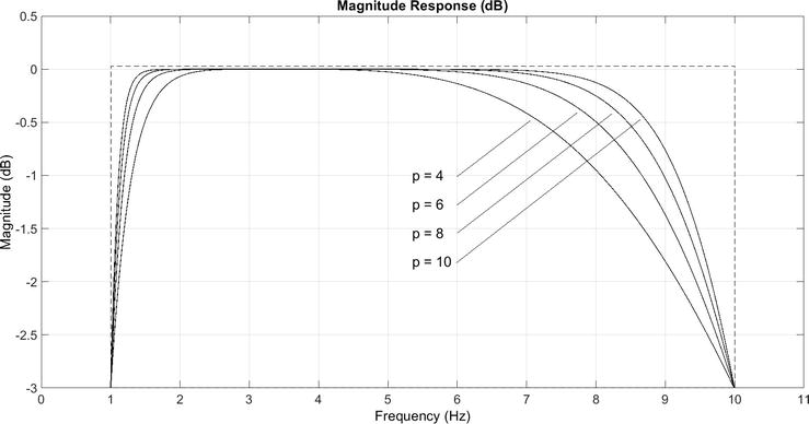
The first condition is satisfied by a digital Butterworth filter with attenuation of 3 dB at the cutoff frequencies corresponding to $f_{\mathit{fl}min}=1\mathrm{Hz}$ and $f_{\mathit{fl}max}=10\mathrm{Hz}$, in which the magnitude–frequency response has the form shown in Figure 5 and depends on the order ($p$) of the digital filter [21]. To satisfy the second condition, it is necessary to analyze the dependencies (Figure 6) of the group delay (${\tau }_{\mathit{\text{delay}}}$) of the measurement results in the specified filter on the frequency.

Figure 5.

Magnitude-frequency response of digital Butterworth filters of various orders.

Figure 6.

Dependence of the group delay of digital Butterworth filters of various orders on frequency.

The output samples of the considered digital Butterworth filter are determined by a general Eq. (21)

$$y_i=\frac{1}{a_0}\left[\sum _{k=0}^p{b}_k{x}_{i-k}-\sum _{k=1}^p{a}_k{y}_{i-k}\right],$$E21

where the number and values of the coefficients $a_k$ and $b_k$ depend on the sampling frequency ($f_s$) of the input data ($x_i$), the filter bandwidth range (limited to values $f_{\mathit{fl}min}$ and $f_{\mathit{fl}max}$) and filter order, which is given by an even integer $p$. In the case of using this filter to process the results of measuring the ionospheric TEC (${\mathit{TEC}}_{\mathit{\text{comb}}}$) in order to evaluate its small-scale fluctuations ($\mathrm{\Delta }{N}_T$), Eq. (21) can be represented as

$$\mathrm{\Delta }{N}_{\mathit{Ti}}=\frac{1}{a_0}\left[\sum _{k=0}^p{b}_k{\mathit{TEC}}_{\mathit{\text{comb}}i-k}-\sum _{k=1}^p{a}_k\mathrm{\Delta }{N}_{\mathit{Ti}-k}\right].$$E22

To justify the choice of the filter order ($p$) for measuring small-scale TEC fluctuations, it should be recalled that, on the one hand, it should have the magnitude–frequency response close to ideal, and on the other hand, it should not introduce a large group delay (${\tau }_{\mathit{\text{delay}}}$) when processing measurement results.

It is known [21] that as the order of the digital Butterworth filter increases, its magnitude-frequency response (Figure 5) approaches the ideal (rectangular) simultaneously with the increase in the group delay (Figure 6). Let us analyze in more detail the dependencies of the group delay (${\tau }_{\mathit{\text{delay}}}$) on the frequency in the range from 1 Hz to 5 Hz (Figure 7).

Figure 7.

Dependence of the group delay of digital Butterworth filters of various orders on the frequency in the range from 1 Hz to 5 Hz.

On the additional vertical axis in Figure 7—the values of the filter delay ${\tau }_{\mathit{\text{delay}}}$ in seconds, on the additional horizontal axis – the period of fluctuations ${\tau }_{\mathit{fl}}$ in seconds. As a criterion for the permissible delay introduced by the filter during the processing of measurement results, we will take a value not exceeding half the period of small-scale TEC fluctuations: ${\tau }_{\mathit{\text{delay}}}\le 0,5{\tau }_{\mathit{fl}}$. In Figure 7, the area of acceptable filter delays is under the dotted curve.

The analysis of Figure 7 shows that the selected criterion for ensuring an acceptable delay in measurement results (${\tau }_{\mathit{\text{delay}}}\le 0,5{\tau }_{\mathit{fl}}$) corresponds to a digital Butterworth filter with the order $p=4$ and $p=6$. Filter with $p=6$, according to Figure 5, has a magnitude–frequency response closer to the ideal, which determines the choice of a digital Butterworth filter with an order $p=6$for estimating small-scale TEC fluctuations. The values of its coefficients ($a_k$, $b_k$) calculated using the digital filter design and analysis software Filter Designer [22] are given in Table 1, and the equation describing this filter can be written as

$k$	$a_k$	$b_k$
0	1	0.076745906902313671
1	−3.4767608600037727	0
2	5.0801848641096203	−0.23023772070694101
3	−4.2310052826910152	0
4	2.2392861745041328	0.23023772070694101
5	−0.69437337677433475	0
6	0.084273573849621822	−0.076745906902313671

Table 1.

Coefficients of the 6th order Butterworth digital filter with a bandwidth from 1 Hz to 10 Hz and a sampling rate of 50 Hz.

$$\mathrm{\Delta }{N}_{\mathit{Ti}}=\sum _{k=0}^6{b}_k{\mathit{TEC}}_{\mathit{\text{comb}}i-k}-\sum _{k=1}^6{a}_k\mathrm{\Delta }{N}_{\mathit{Ti}-k}.$$E23

Figure 8 shows the results of the evaluation of small-scale TEC fluctuations ($\mathrm{\Delta }{N}_T$) in accordance with Eq. (23), expressed in $\text{TECU}={10}^{16}{\mathrm{m}}^{-2}$ units. These results were obtained at the North-Caucasus Federal University (Stavropol, Russia) using the advanced capabilities of the GPStation-6 receiver.

Figure 8.

Small-scale TEC fluctuations at the output of the digital filter.

Thus, to evaluate (isolate) the small-scale TEC fluctuations ($\mathrm{\Delta }{N}_T$), it is advisable to use a 6th-order Butterworth digital filter, the output samples of which are formed according to the obtained Eq. (23). Digital filter, with values of minimum and maximum transmission frequencies $f_{\mathit{fl}min}=1\mathrm{Hz}$ and $f_{\mathit{fl}max}=10\mathrm{Hz}$ and sampling frequency $f_s=50\mathrm{Hz}$, provides a magnitude–frequency response close to ideal (Figure 5) with an acceptable value (${\tau }_{\mathit{\text{delay}}}\le 0,5{\tau }_{\mathit{fl}}$) of the delay introduced by it (Figure 7). To implement a digital Butterworth filter with the specified parameters its coefficients ($a_k$ and $b_k$) are calculated using the digital filter design and analysis tool (Filter Designer) and are shown in Table 1.

5. Use of results of GPS monitoring of small-scale fluctuations of the total electronic content of the ionosphere for prediction of the noise immunity of the satellite communication system

Figure 9 shows the simplest case of using the results of GPS monitoring of small-scale TEC fluctuations to predict the noise immunity of the SCS, when the trans-ionospheric radio wave propagation from the GNSS satellite (with carrier frequencies $f_1$ and $f_2$) and from the SCS satellite (with carrier frequency $f_0$) to the GPStation-6 receiver occurs at the same elevation angle ($\alpha \ge {30}^{\circ }$).

Figure 9.

The structure of the construction of the modified GPStation-6 receiver for the evaluation of the RMS of small-scale TEC fluctuations (${\sigma }_{\mathrm{\Delta }{N}_T}$), scintillation index ($S_4$), and the error probability ($P_{\mathit{err}}$) when receiving SCS signals.

In order to estimate the noise immunity of SCS based on small-scale TEC fluctuations ($\mathrm{\Delta }{N}_T$) it is necessary to modify software of GPStation-6 receiver (Figure 3) by adding three units (Figure 9): RMS (${\sigma }_{\mathrm{\Delta }{N}_T}$) calculation unit, scintillation index ($S_4\sim {\sigma }_{\mathrm{\Delta }{N}_T}/f_0$) calculation unit, and error probability ($P_{\mathit{err}}\sim S_4$) calculation unit.

Small-scale TEC fluctuations (Figure 8) at the output of the digital filter (Eq. (23)) can be characterized by zero mathematical expectation $\overline{\mathrm{\Delta }{N}_T}=0$ and the RMS

$${\sigma }_{\mathrm{\Delta }{N}_T}=\sqrt{\frac{1}{n}\sum _{i=1}^n{\left(\mathrm{\Delta }{N}_{\mathit{Ti}}-⟨\mathrm{\Delta }{N}_T⟩\right)}^2}=\sqrt{\frac{1}{n}\sum _{i=1}^n\mathrm{\Delta }{N}_{\mathit{Ti}}^2}.$$E24

on the measurement interval ${\tau }_{\mathit{RMS}}=t_n-t_1=1\mathrm{s}$, during which the average (background) value of the TEC (${\overline{N}}_T$) can be considered unchanged. The specified measurement interval ${\tau }_{\mathit{RMS}}={\tau }_{s}n=1\mathrm{s}$ corresponds to $n=50$ samples with a sampling interval ${\tau }_s=0.02\mathrm{s}$ (sampling frequency $f_s=1/{\tau }_s=50\mathrm{Hz}$).

The results of the calculation in accordance with Eq. (24) of the RMS (${\sigma }_{\mathrm{\Delta }{N}_T}$) of the small-scale TEC fluctuations ($\mathrm{\Delta }{N}_T$) obtained at the output of the digital filter (Figure 8) are shown in Figure 10.

Figure 10.

RMS of the small-scale TEC fluctuations.

The analysis of Figures 8 and 10 shows that at about 12:56:40 local time (UTC + 3) there was a sharp short-term increase in small-scale TEC fluctuations (with RMS up to ${\sigma }_{\mathrm{\Delta }{N}_T}\approx 0.05\text{TECU}$). It coincides with the moment when the received GLONASS signals scintillation occurs (Figure 2). This generally confirms the dependence of the ionospheric scintillation index ($S_4\sim {\sigma }_{\mathrm{\Delta }{N}_T}$) on the RMS (${\sigma }_{\mathrm{\Delta }{N}_T}$) of small-scale TEC fluctuations. In the considered interval, it is ${\sigma }_{\mathrm{\Delta }{N}_T}\approx 0.02\text{TECU}$ on average, which is consistent with the known [5, 6, 8, 10] data on the magnitude of relative TEC fluctuations of the mid-latitude ionosphere at typical values of the average TEC ${\overline{N}}_T\approx 10\text{TECU}$: ${\sigma }_{\mathrm{\Delta }{N}_T}/{\overline{N}}_T\sim {\sigma }_{\mathrm{\Delta }N}/{\overline{N}}_m<{10}^{-3}{\mathrm{...10}}^{-2}$. This confirms the reliability of the obtained results of filtration of small-scale TEC fluctuations.

Figure 11 shows calculation results of the scintillation index ($S_4$) of the received signal in the typical SCS (with carrier frequency $f_0=1.6\mathrm{GHz}$) in accordance with Eq. (6) based on the results of the evaluation of the RMS (${\sigma }_{\mathrm{\Delta }{N}_T}$) of small-scale TEC fluctuations (Figure 10).

Figure 11.

Scintillation index of received SCS signals with carrier frequency $f_0=1.6\mathrm{GHz}$.

The results of the scintillation index calculating in accordance with Eq. (6) shown in Figure 11 are corresponding to the results shown in Figure 2 (bottom panel). This allows us to conclude that the dependence (Eq. (6)) is reliable. However, unlike the results of calculating the scintillation index by the built-in GPStation-6 receiver software (bottom panel in Figure 2), the results shown in Figure 11 have two advantages:

1) as initial data for the calculation of the scintillation index $S_4$ (Eq. (6)), the results of the evaluation of the RMS (${\sigma }_{\mathrm{\Delta }{N}_T}$) of small-scale TEC fluctuations are used. It characterizes the cause of the scintillation - small-scale ionospheric irregularities. Multiple reflection of radio waves from objects surrounding the receiving antenna has no effect on the results of calculating the scintillation index;

2) the results of the evaluation of the RMS (${\sigma }_{\mathrm{\Delta }{N}_T}$) of small-scale TEC fluctuations and the results of the scintillation index $S_4$ (Eq. (6)) calculation are formed with a sampling interval ${\tau }_s=1\mathrm{s}$. This makes it possible to register an increase in the scintillation index when short-term (units of seconds) ionospheric scintillation occur.

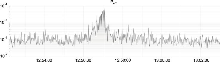
The monitoring data of the RMS (${\sigma }_{\mathrm{\Delta }{N}_T}$) of small-scale TEC fluctuations allow us to predict changes in the noise immunity of SCS based on Eq. (6) $S_4\sim {\sigma }_{\mathrm{\Delta }{N}_T}/f_0$ and Eq. (7) $P_{\mathit{err}}=\psi \left(S_4,⟨h^2⟩\right)$. The results of calculating the probability of error ($P_{\mathit{err}}$) when receiving SCS signals with an average signal-to-noise energy ratio $⟨h^2⟩=12\mathrm{dB}$ at the receiver input are shown in Figure 12.

Figure 12.

Probability of error when receiving SCS signals.

The analysis of Figure 12 shows that in the conditions of an undisturbed mid-latitude ionosphere, high noise immunity of the typical SCS is provided. It is characterized by the magnitude of the error probability when receiving signals $P_{\mathit{err}}\approx {10}^{-6}$. At the moment of the occurrence of weak ionospheric scintillation value of the error probability briefly increased up to $P_{\mathit{err}}\approx {10}^{-5}{\mathrm{...10}}^{-4}$ (by 1–2 order of magnitude). This confirms, that under conditions of natural disturbances of the ionosphere in polar and equatorial regions, the error probability may significantly increase and exceed the permissible value (its traditional value is $P_{\mathit{err}}\le {10}^{-5}$ according to [8]).

The experimental data obtained (Figures 10–12) confirm the dependence of the error probability ($P_{\mathit{err}}\sim S_4\sim {\sigma }_{\mathrm{\Delta }{N}_T}/f_0$) when receiving elementary symbols of messages in SCS on the RMS (${\sigma }_{\mathrm{\Delta }{N}_T}$) of small-scale TEC fluctuations and the choice of carrier frequency ($f_0$). Ionospheric disturbances accompanied by the formation of small-scale irregularities (and an increase in small-scale TEC fluctuations ${\sigma }_{\mathrm{\Delta }{N}_T}$) can lead to an increase in the error probability ($P_{\mathit{err}}\sim S_4\sim {\sigma }_{\mathrm{\Delta }{N}_T}/f_0$) in SCS using the low-frequency range ($f_0=\mathrm{0.2...0.4}\mathrm{GHz}$) by more than 2 orders of magnitude (up to $P_{\mathit{err}}={10}^{-3}{\mathrm{...10}}^{-1}$).

6. Conclusion

A method has been developed for GPS monitoring of small-scale fluctuations of the ionospheric TEC and their use for predicting changes in the noise immunity of SCS during ionospheric disturbances. It is based on digital filtering of small-scale fluctuations of the TEC of the ionosphere and evaluation of their RMS.

The software of the GPStation-6 receiver has been modified (Figure 3) in the direction of replacing the TEC code measurements with combined (code-phase) measurements, which eliminates noise component of measurement error.

To isolate small-scale TEC fluctuations, it is proposed to use a 6th-order digital Butterworth filter, which at reasonable extremes of the transmission frequency range (1 Hz, 10 Hz) and sampling frequency (50 Hz), provides magnitude–frequency response close to ideal (Figure 5) and introduces a delay that does not exceed the permissible level (Figure 7). It is described by Eq. (23) and Table 1.

The obtained results of the evaluation of small-scale TEC fluctuations at the output of the digital filter (Figure 8) allow (in accordance with Eq. (24), Eq. (6), and Eq. (7)) to consistently obtain an estimate of the RMS of these fluctuations (Figure 10), the ionospheric scintillation index (Figure 11) and the probability of error when receiving elementary symbols of SCS messages (Figure 12).

Acknowledgments

The work was carried out with the support of the Russian Science Foundation within the scientific project No. 22-21-00768 (https://rscf.ru/project/22-21-00768) “Methodology for the construction of structural and physical models of trans-ionospheric radio channels and their application to the analysis of satellite radio systems during ionospheric scintillation”.

References

1.Recommendation ITU-R P.531-14. Data on ionospheric propagation data and prediction methods required for the design of satellite services and systems [Internet]. 2020. Available from: https://www.itu.int/dms_pubrec/itu-r/rec/p/R-REC-P.531-14-201908-I!!PDF-R.pdf
2.Yeh KC, Liu CH. Radio wave scintillations in the ionosphere. Proceedings of the IEEE. 1982;70(4):324-360
3.Crane RK. Ionospheric scintillation. Proceedings of the IEEE. 1977;65(2):180-199
4.Aarons J. Global morphology of ionospheric scintillations. Proceedings of the IEEE. 1982;70(4):360-378
5.Kravtsov YA, Feyzulin ZI, Vinogradov AG. Propagation of Radio Waves through the Earth Atmosphere. Moscow: Radio i Svyaz; 1983
6.Cherenkova E, Chernyshev O. Propagation of Radio Waves. Moscow: Radio i Svyaz; 1984. p. 272
7.Davis K. Radio Waves in the Ionosphere. Moscow: Radio i Svyaz; 1973
8.Maslov ON, Pashintsev VP. Models of transionospheric radio channels and noise immunity of space communication systems. Appendix to the Journal Infocommunication Technologies. 2006:4
9.Pashintsev VP, Peskov MV, Kalmykov IA, Zhuk AP, Toiskin VE. Method for forecasting of interference immunity of low frequency satellite communication systems. AD ALTA: Journal of Interdisciplinary Research. 2020;10(1):367-375
10.Ryzhkina TE, Fedorova LV. Investigation of static and spectral transatmospheric VHF-microwave radio signals. Journal of Radio Electronics. 2001;2001:2 Available from: http://jre.cplire.ru/win/feb01/3/text.html
11.Afraimovich EL, Perevalova NP. GPS monitoring of the earth upper atmosphere. Irkutsk. 2006;2006:480
12.Perevalova NP. Evaluation of the characteristics of a ground-based GPS/GLONASS receiver network designed to monitor ionospheric disturbances of natural and technogenic origin. Solar-terrestrial Physics. 2011;19:124-133
13.Rytov SM, Kravtsov YN, Tatarsky VI. Introduction to Statistical Radiophysics. Vol. 22. Moscow: Nauka; 1978. p. 464
14.Fremouw EJ, Leadabrand RL, Livingston RC, Cousins MD, Rino CL, Fair BC, et al. Early results from the DNA wideband satellite experiment-complex-signal scintillation. Radio Science. 1978;13(1):167-187
15.Popov VF. Evaluation of the noise immunity of spaced signals reception in the channel with fading according to the Nakagami law and coherent weight addition. Omskiy Nauchny Vestnik. 2012;3(113):309-313
16.Demyanov V, Yasyukevich Y. Space weather: Risk factors for global navigation satellite systems. Solar-Terrestrial Physics. 2021;7(2):28-47
17.Shanmugam S, Jones J, MacAulay A, Van Dierendonck AJ. Evolution to modernized GNSS ionoshperic scintillation and TEC monitoring. In: Proceedings of IEEE/ION Position, Location and Navigation Symposium (PLANS) [Internet]. IEEE; 2012. pp. 265-273. Available from: https://ieeexplore.ieee.org/document/6236891
18.GPStation-6. GNSS Ionospheric Scintillation and TEC Monitor (GISTM) Receiver User Manual [Internet]. 2012. Available from: https://hexagondownloads.blob.core.windows.net/public/Novatel/assets/Documents/Manuals/om-20000132/om-20000132.pdf
19.Carrano CS, Groves KM. The GPS segment of the AFRL-SCINDA global network and the challenges of real-time TEC estimation in the equatorial ionosphere. In: Proceedings of the 2006 National Technical Meeting of The Institute of Navigation, Monterey, CA. Manassas, VA: ION; 2006. pp. 1036-1047
20.OEM6. Firmware Reference Guide [Internet]. 2014. Available from: https://hexagondownloads.blob.core.windows.net/public/Novatel/assets/Documents/Manuals/om-20000129/om-20000129.pdf
21.Bogner RE, Constantinides AG. Introduction to Digital Filtering. London: A Wiley-Interscience Publication; 1975. p. 212
22.MathWorks. Filter Designer [Internet]. The MathWorks, Inc. 2020. Available from: https://www.mathworks.com/help/signal/ref/filterdesigner-app.html
Written By
Vladimir Pashintsev, Mark Peskov, Dmitry Mikhailov, Mikhail Senokosov and Dmitry Solomonov
Submitted: 23 December 2022Reviewed: 11 January 2023Published: 28 February 2023
Open access peer-reviewed chapter