Improving the Accuracy of the Global Navigation Satellite System

Abstract

The ionosphere influences satellite navigation and communication significantly because it behaves like a dispersive medium. As the density of free electrons increases, so does the influence, and vice versa. The concentration of the electron density in the ionospheric layer causes delays that affect the accuracy and reliability of Global Navigation Satellite Systems. Therefore, studying the ionospheric characteristics, variations of the electron density in certain regions, and ionospheric models are crucial when assessing the quality of ionospheric models. These are useful in determining the suitability of the models to improve the accuracy of the global navigation system.

1. Introduction

Global navigation satellite signals are heavily influenced by the environment in space and the Earth’s atmosphere because they emanate from satellites at an elevation of around 20,000 km from the Earth to receiving satellites on the surface [1]. The ionosphere extends from approximately 60–1500 km above the surface of the Earth, making it the upper layer of the atmosphere at the edge of space that affects radio communication satellite systems. Within the ionosphere, some solar radiation frequencies are absorbed, resulting in the separation of neutral gas atoms or molecules into free electrons and ions [2], a process known as ionization. The extent to which ionization occurs depends mainly on solar activity and the geomagnetic field. The free electrons and ions from the process interact with microwaves, such as Global Navigation Satellite Systems (GNSS) signals, affecting their propagation velocity and causing a delay of up to several meters in the zenith direction. This process depends on the latitudinal and longitudinal coordinates of the sun-fixed coordinate system, making ionospheric delay important when considering the accuracy of GNSS signals.

GNSS uses one or more frequencies to transmit various signals and navigation data. These signals vary in their availability and dependability. GNSS single-frequency receivers collect satellite radio signals on one frequency and are the most common type of receiver, making them cost-effective but unable to estimate ionospheric delay. Conversely, dual-, triple-, and multi-frequency receivers can collect radio signals from GNSS at a minimum of two frequencies, respectively. Multi-frequency GNSS receivers can estimate ionospheric delays and remove their effects; however, they are used in specialized research areas. Generally, single-frequency is significantly better than dual-frequency in terms of accuracy and cost, a single-frequency receiver may give you decimeters of accuracy within minutes while a dual-frequency receiver may take as long as 20–40 min to reach centimeters of accuracy. Additionally, the single-frequency receiver can outperform the dual-frequency receiver in areas known to have a frequent loss of lock in the signals [3].

2. Global navigation satellite system

GNSS is a satellite constellation revolving around the earth, broadcasting radio signals from within space to GNSS receivers, carrying data for timing and positioning. The system allows receivers to discover their positions within a few meters employing time signals transmitted with satellite radio signals in a linear path. This allows the system to provide global coverage. It comprises three components: the space component (including the constellation of satellites and their movement in space), the control component (which aims to manage the system and owner), and the user component (which consists of the GNSS receivers and user interfaces).

GNSS is classified into two groups: GNSS-1 and GNSS-2. The former is known as first-generation systems that combine the Ground-Based Augmentation (GBA) System or the Satellite-Based Augmentation System (SBAS) with the current satellite navigation system (GLONASS and GPS). Some real-world applications are in the Multi-Functional Satellite Augmentation System (MSAS) used in Japan, the Wide Area Augmentation System (WAAS), a component that is satellite-based in the US, and the European Geostationary Navigation Overlay System (EGNOS) in Europe. On the other hand, GNSS-2, of which the European GALILEO positioning system is an example of a second-generation system that provides a total civilian satellite navigation system. These systems provide the integrity monitoring and accuracy needed for civil navigation. GNSS is the collective consultation of the Global Navigation Satellite System (GLONASS) created by Russia, the Navigation System with Timing and Ranging (NAVSTAR) Global Positioning System (GPS) created in the United States, the Quasi-Zenith Satellite System (QZSS) created in Japan, the Galileo created by the European Union, and the BeiDou developed by China.

GPS is an example of an Intermediate Circular Orbit (ICO) satellite navigation system. The US government’s Department of Defense (DoD) developed it in 1973 to assist the military. It is the oldest and most accurate GNSS in the world [4]. The system operates in an L-Band frequency having a radio spectrum between 1 and 2 GHz. The most recent GPS satellite generations employ rubidium clocks with an accuracy of ±5 parts in 1011. More precise ground-based cesium clocks are used to synchronize the rubidium clocks.

3. GNSS/GPS signal structure

Precise cesium or rubidium atomic clocks that oscillate at a fundamental frequency of 10.23 MHz are used to produce the GNSS/GPS satellite signal. The satellites transmit signals on two L-band carrier frequencies, L1 = 1575 MHz and L2 = 1227.60 MHz. The L1 carrier is modulated with two codes: the coarse-acquisition code (C/A) at 1.023 MHz and the precise code (P) at 10.23 MHz. On the other hand, Figure 1 shows the L2 carrier having only one modulated code, the P-code at 10.23 MHz.

Figure 1.

GPS satellite signals. Source: Khan et al. [5].

The two types of GNSS position determination codes consist of pseudo-random noise (PRN). This noise plays a significant role in the position-determination technique. When modulated on the L1 and L2 carriers, it produces a jam-resistant spread-spectrum signal. Once the anti-spoofing (AS) operation mode is enabled, the P-code may be encrypted into a Y-code. The P-code repeats weekly, beginning at the start of the GPS week, while the C/A code repeats every millisecond. There is also the navigation message, which is modulated with the L1 and L2 carriers at a chip rate of 50 bps. It contains data on ionospheric parameters, perturbations in orbit, satellite orbits, GPS time, satellite clocks, and messages about the system’s status. [6]. The quadrature phase-shift keying (QPSK) scheme is used to modulate L1 with P-code, C/A-code, and navigation messages.

To extend the capability of the GNSS, particularly the GPS, it was modernized to give added benefits to the civilian signal. Three new civilian signals, L2C, L5, and L1C, were introduced into the new military signal (M) on the L1 and L2 frequencies. In a dual-frequency receiver, the concurrent use of the L1 C/A (first civilian) and L2C (second civilian) enables ionospheric correction, and enhancing its accuracy in comparison to the military signal. The receivers will increase in complexity in the coming years to support tracking of the new civil code on L2 and the encrypted P on L2 (A-S). L5 has a frequency of 1176.45 MHz and a chipping rate of 10.23 MHz. The L5 code’s high chipping rate will provide high-performance ranging capacities as well as better code measurements than L1 C/A code measurements [7]. However, both old and new civil and military codes require improved modulation to better share current frequency allocations with all signals by raising spectral separation and thereby conserving the spectrum. The binary offset carrier (BOC) can then be used to modulate military codes [8].

4. GNSS/GPS observables

There are two fundamental signals in GNSS/GPS observables: carrier phase and pseudorange (code). Pseudoranges are used in high-precision positioning and navigation, where the carrier phase is preferred. Phase observation has the advantage of lower noise but has at least one extra unknown parameter for each satellite, meaning the integer’s ambiguity has to be introduced. The difference between the phase of the carrier signal produced by the receiver at the time of signal reception and the phase of the satellite signal produced at the time of signal transmission is known as the ambiguous range or the carrier phase. The initial observation only involves the fractional part of the phase difference. As tracking continues without a cycle slip, the receiver keeps track of the fractional part and the number of cycles. Ambiguity occurs because the measurement does not include the initial number. The carrier phase is typically determined in cycles and can be converted to length units by multiplying it by the wavelength at operational frequencies. Thus, Eq. (1) defines the carrier-phase equation in length units. The pseudorange is the distance between the satellite and the receiver at the start of the code’s transmission and reception. It is scaled using a vacuum’s nominal speed of light. Timing errors and delays with the GNSS time in the receiver and satellite clocks will differentiate the measured pseudoranges from the LOS, which corresponds to the beginning of transmission and reception. Eq. (2) shows the pseudorange’s mathematical expression, and Table 1 depicts the main characteristics of the carrier phase and the code.

	Carrier	Code
Propagation effects ambiguity	Ambiguous	Unambiguous
Wavelength	20 cm	P-code 30 m; C/A-code 293 m
Observation noise	2 mm	P-code 30 cm; C/A-code 3 m
Accuracy	High accuracy	Low accuracy

Table 1.

The carrier phases and code characteristics.

$${\varphi }_r^s={\rho }_r^s+c\left(\delta t_r-\delta t^s\right)-I+T+\lambda N_r^s+\mathit{mp}+\epsilon$$E1

$$P_r^s=c\left(t_r-t^s\right)=c{\tau }_r^s={\rho }_r^s+c\left(\delta t_r-\delta t^s\right)+I+T+\mathit{mp}+\epsilon$$E2

where ${\varphi }_r^s$ is the phase measurement in units of length. $P_r^s$ is the pseudorange measured at the receiver. c is the speed of light in a vacuum. $\delta t_r\wedge \delta t^s$ are the satellite and receiver clock errors due to the difference in system time. I is the ionospheric-induced error. T is the tropospheric-induced error. $N_r^s$ is integer ambiguity between the satellite and receiver. $\lambda$ is the wavelength. $\mathit{\text{mp}}$ is the multipath error. $\epsilon$ is the noise or random error, $t_r$ is the reception time of the signal measured by the clock of receivers r, $t^s$ is the transmission time of signal measured by the time frame of satellite s, and ${\tau }_r^s$ is the signal traveling time.

Noise or error sources that might be included in the observables are orbital errors, antenna phase center offsets, and receiver noise, which should be considered for measurement accuracy. When the geomagnetic field effect and path bending are ignored, the phase advance is identical to the ionospheric-induced group delay’s magnitude. Although they contain ambiguities, the phase observations are two to three orders of magnitude more accurate compared to the pseudorange code. The LOS range between satellite coordinates (X^s, Y^s, Z^s) and receiver coordinates (x_r, y_r, z_r) is provided as:

$${\mathit{\rho }}_{\mathit{r}}^{\mathit{s}}\mathit{=}\sqrt{{\left({\mathit{X}}^{\mathit{s}}\mathit{-}{\mathit{x}}_{\mathit{r}}\right)}^{\mathbf{2}}\mathit{+}{\left({\mathit{Y}}^{\mathit{s}}\mathit{-}{\mathit{y}}_{\mathit{r}}\right)}^{\mathbf{2}}\mathit{+}{\left({\mathit{Z}}^{\mathit{s}}\mathit{-}{\mathit{z}}_{\mathit{r}}\right)}^{\mathbf{2}}}$$E3

5. Doppler shift

The Doppler shift of a GNSS signal is the carrier phase’s derivative of time. It is primarily given by the antenna’s relative velocity at the satellite and receiver, and the common offset, which is proportional to the error in the receiver clock’s frequency. In order to receive and accept the signals, the GNSS receiver has to estimate the Doppler shift of the signals.

6. GNSS observable errors

Errors and noise caused by the propagation of a signal through atmospheric layers and noise measurements have an impact on phase and code measurements. These errors are classified into three types: satellite-based errors (including satellite clock biases and ephemeris), receiver-based errors (including receiver clock errors, inter-channel biases, and receiver noise), and propagation errors (including tropospheric and ionospheric delays, multipath signals, and other interferences). The main GNSS observable errors are described as follows:

6.1 The satellite-based error

The clock’s errors are caused by time differences between the satellite clock and the real GNSS. The transmitted navigation message from the satellite includes some corrections for clock drifts, resulting in positional errors. Satellite clock errors are typically less than 1 msec, which equates to a 300 km error in pseudorange that can be removed by the difference between two receivers based on their respective satellites. Errors in the receiver clocks are significantly bigger than those in satellite atomic clocks because they use inexpensive crystal clocks with reduced precision. Depending on the firmware of the receiver, the size of the receiver clock error will range between 200 ns and some milliseconds. The clock’s errors can be eliminated with the difference between the same receiver of two satellites [9]. It is possible to model this using the navigation message carrying a reference time and containing the polynomial coefficients transmitted.

The errors in satellite ephemeris are caused by inaccurate satellite position predictions that are transmitted in a navigation message to users. The satellite’s position is dynamic and depends on the solar pressure and gravitational field. The calculation of position by a ground master control station is susceptible to error because of the monitoring station’s clock drifts and delays. Errors in estimating the position of the satellite result in pseudorange errors, which must be corrected at the level of the user.

6.2 The receiver-based error

A receiver clock’s error occurs because non-precise clocks are used, causing an offset between it and the GNSS reference time. These errors are regarded as unknowns in the pseudorange calculations. However, the double difference equation can be used to remove them, as shown in the following section [6].

The interchange bias is the correlated error that is caused by the internal GNSS receiver processes. It cannot be measured with live data because large errors in the GNSS measurements make the bias impossible to measure because it is much smaller. The only way it can be measured is to zero out all other channels of error. This can be done using a GNSS simulator [10]. In addition, the biases in GNSS positioning occur because of physical limitations and inadequacies in the hardware of the GNSS. They are caused by little delays between actions that should be run concurrently when signals are transmitted via satellite or acquired using a receiver [11]. Furthermore, receiver noise, also known as random measurement noise, influence carrier-phase measurements and code delay. This noise is unrelated to the signal. Noise is produced by the cables, amplifiers, antennae, and the receiver itself. The random measurement noise includes interference from other GNSS signals. Even though the error contributes only a minor portion of overall positioning, it has been improved with modern GNSS receiver technology.

6.3 Propagation error

Multipath occurs when the satellite or receiver gets multiple signal reflections because of the numerous paths the signal takes to reach its destination. The multipath effect depends on the satellite’s geometry, the reflecting surfaces surrounding the receiving antenna, and the antenna’s position. Signals received from higher-altitude satellites are less susceptible to the multipath effect than those received from low-angle ones. Multipath errors affect the pseudorange measurement much more than they do the carrier phase because of frequency dependency. To reduce multipath errors, a site far from any reflective surfaces (trees, buildings, mounting, and cars) should be selected. Multipath errors, on the other hand, can reach 1 m and can be removed with antennas that use signal polarization to their advantage. The troposphere is the lowest region in the atmosphere where all weather phenomena take place. The GNSS signals are affected by tropospheric attenuation. The tropospheric layer triggers a delay in carrier and code observations that the dual-frequency receiver cannot remove. However, the tropospheric delay can be modeled successfully. Tropospheric models rely on empirical models that take temperature, relative humidity, mapping function, and pressure values into account [12].

The ionosphere is the uppermost layer of the atmosphere, and it contains a large amount of free ions and electrons. GNSS signals are refracted and dispersed nonlinearly in the ionosphere by free electrons. The ionosphere’s dispersive nature causes the delays to become dependent on frequency. The number of free electrons passing through the path of the signal ray is proportional to the total ionospheric delay, which varies depending on the time of day, year, solar cycle, and geographic location on and above the Earth’s surface [13]. For the GNSS signal frequency receiver, the Klobuchar model can only remove about 50 to 60% of the ionospheric errors. Additionally, users of single-frequency GNSS can use empirical ionospheric models or the regional network via communication links using real-time correction. Ionospheric errors on signals received from GNSS satellite signals play the greatest role in positioning errors when using single-frequency GNSS receivers. These phenomena become obvious during severe solar activity, such as geomagnetic storms. For any radiometric space method, like those using the GNSS system, it is imperative to give an account of the propagation delay that emanates from the neutral atmosphere. As the ionosphere is the primary error source in GNSS single-frequency measurements, understanding its variations and properties, as well as identifying accurate ionospheric delay approaches, is critical to improving its accuracy. However, ionospheric errors can be partially eliminated using the linear combination of dual or multiple frequencies [14].

7. Ionospheric total electron content

The total electron content (TEC) is defined by the integral of the electron density in a TEC unit (TECU), where one TECU is equal to 1016 electrons per square meter along the signal transmission path to the receiver. The TEC significantly affects electromagnetic waves that propagate through the ionosphere. TEC is measured using dual-frequency GNSS receivers, which is a popular method for investigating the dynamics of the ionosphere [15]. As a result, the study of the TEC gained a new impetus with GPS-based ground and navigation positioning that makes use of trans-ionospheric communication. As the TEC depends significantly on the state of the ionosphere, it has a large effect on GNSS-based communications. The ionospheric delay varies substantially with the geographical location (equatorial, low-latitude, mid-latitude, and high-latitude regions). However, due to the unique geometry of the magnetic field, the ionospheric delay is obvious in low-latitude and equatorial regions. In such regions, the plasma density in the ionosphere shows significant variations. These variations are influenced by the solar cycle, geomagnetical activities, time of day, seasons, and geographical location [16].

8. Ionospheric regions

The ionosphere is classified into three major regions: the equatorial/low-latitude, mid-latitude, and high-latitude regions. In high-latitude regions, the electron density is significantly lower than in low-latitude regions because solar radiation hits the atmosphere more aggressively there. In mid-latitude regions, ionization occurs due to solar photon radiation, with the electron density not being subject to any particle radiation. In equatorial or low-latitude regions, there is a high electron density concentration because of the high radiation from the sun coupled with the electric and magnetic fields of the earth. Hence, the results of the accumulated electrons in this region influence radio wave propagation, which significantly affects satellite communication systems.

9. Major ionospheric variations

The ionospheric variability is influenced by solar radiation because of photoionization from the sun. Photoionization is caused by the increase in electron density in the ionosphere. The TEC is affected by the activity of the sun, reaching its maximum value when there is high solar activity and decreasing during low solar activity. The sunspot number is one of the indicators commonly employed to determine solar activity. Additionally, the electron density is expected to be higher than that in other locations because of the change in latitude away from the equator and the oblique angle at which solar radiation arrives in the atmosphere. This results in the reduction of ionospheric densities. Geographical locations with low zenith angles are exposed to more solar radiation, hence the higher electron densities. Moreover, maximum electron density occurs during the day and becomes lower at night since there is no photoionization because of the absence of solar radiation. In general, when photoionization stops, recombination significantly reduces the electron density at night, but some free electrons remain until dawn. This variation can appear clearly in equatorial regions. Emunim et al. [16] investigated the daily variation of ionospheric delay at different stations in equatorial regions (UUMK with geographic coordinates at 4.62°N–103.21°E, MUKH with geographic coordinates at 6.46°N to 100.50°E, and TGPG with geographic coordinates at 1.36°N–104.10°E) during a typically quiet day (Kp ≤ 1) on 7 March 2013. As shown in Figure 2, the hourly median local time (Malaysia local time = universal time + eight hours) was charted with the Vertical TEC (VTEC) represented on the horizontal and vertical axes, respectively. The daily pattern of ionospheric delay was observed as a single peak. The general ionospheric delay over all the stations showed that the smallest delay was observed at sunrise, from 4:00 to 6:00 LT. From 13:00 to 17:00 LT, it increased gradually to a maximum. Variations in the solar EUV caused a steady increase in delay, where increased EUV led to increased ionization, which in turn increased the delay and vice versa.

Figure 2.

The diurnal hourly variation of the ionospheric delay. Source Elmunim et al. [16].

Additionally, looking at seasonal variations, during the equinox months, the electron densities increased, because the sun was directly overhead at the equator during solar maximum and minimum activities, leading to an increase in electron density compared to other seasons. Direct sunlight in equatorial regions in equinoctial months causes the most ionization in the ionosphere. The summer had the shortest ionospheric delay, which could be due to uneven heating of the two hemispheres caused by transporting neutral substances from the summer to the winter hemisphere (hot to cold). This reduces the rate of recombination during the winter in comparison to the summer, resulting in a significant rise in the concentration of electrons during the winter. Another possible cause of this phenomenon is a shift in the path of the neutral wind. As it blows in reverse to the plasma diffusion process that begins at the equator, the meridional component of the neutral wind blows from the summer to the winter hemisphere, lowering the ionization crest value in the summer solstice. This results in the equinox meridional winds originating at the equator blowing toward the poles, causing the ionization crest value to be high [17]. An example of the seasonal variation in equatorial regions is discussed in Ref. [18], where Langkawi station was used at geographic coordinates 6.19°N, 99.51°E in 2014. The variabilities of the ionospheric delay (VTEC) during winter (January, February, November, and December), summer (May, June, July, and August), and equinox (March, April, September, and October) are described in Figure 3, where the maximum variation in all the seasons was observed from 9:00 to 19:00 LT. The peak was obtained during the equinox, followed by winter, and finally summer.

Figure 3.

The seasonal variation of the ionospheric delay.

Furthermore, during geomagnetic storms, the ionospheric delay affects GNSS signals because of energy input into the polar ionosphere, changing a few of the thermosphere’s parameters, such as composition, temperature, and circulation. This change in composition influences the concentration of electrons in the F2 region directly, followed by the TEC as the heated gas is spread to lower latitudes through circulation [19]. During severe geomagnetic storms, currents in the dusk-to-dawn direction that are associated with inner magnetospheric electric fields are no longer able to shield the equatorial and mid-latitudes from the electric fields of high latitude. This causes electric fields to penetrate the ionosphere from high latitudes to the equatorial and middle ionosphere in an instant. So, the transportation of the particles and the instantaneous penetration of the high-latitude electric field toward the equator at high velocities can increase the ionospheric delay and the TEC value [20].

However, this complex nature of the equatorial ionosphere has been of great concern due to the large errors that are peculiar to the GNSS applications [20]. The delay errors are attributed to the free electrons in the signal path. The variations in the value of the TEC need to be considered in the equatorial region so that the accuracy of the GNSS can be improved. Studying the variations in the TEC at different geographical locations under various geophysical conditions like geomagnetic storms is also crucial. Therefore, it is essential to develop a suitable ionospheric model to minimize GPS positioning errors.

Research has been done on different low-latitude and equatorial regions of the world using GNSS. Researchers have documented concerns in the analysis of GPS-TEC variations in a particular ionospheric region at a specific time. For instance, as discovered by Bagiya et al. [21], semiannual variations with maximum values were recorded between March and April and again between September and October. Furthermore, they reported that seasonal variations in the TEC at night show a semiannual periodicity, with high background levels during the equinoctial months and low background levels during the solstices. Tariku [22] discovered that the lowest and highest monthly values of ionospheric delay were seen during the June solstice and the equinoctial months, respectively, from 2009 to 2011 over the Kenyan region.

Shimeis et al. [23] studied the temporary variations of the ionospheric delay at some stations in Africa from 2002 to 2012. They observed that the ionospheric delay’s daily variation gave multiple maxima in the summer equinox between 2006 and 2012 and during the equinox months from 2005 to 2008. Based on their report, increasing nighttime VTEC and winter irregularities were observed during the study period. They also reported that, during the time of a deep solar minimum (2006–2009), during a quiet period of geomagnetic activity in the equatorial latitudes, a similar diurnal variation of the ionospheric delay was observed over Alexandria (Egypt). Akala et al. [23] compared equatorial GPS-TEC data from an American and an African station during the ascending and descending phases of the solar cycle 24. The study revealed that the minimum and maximum seasonal values of the ionospheric delay were reported during the solstices and the March equinox, in the solar minimum phases of both stations. Meanwhile, during the ascending phase of solar activity, the June solstice had the lowest values and the December solstice had the highest values. Huy et al. [24] investigated the time variations of the ionospheric delay in Southeast Asian equatorial ionization anomalies from 2006 to 2011. Their findings also revealed that crest amplitude ionization was significantly reduced in a few months during the winter and summer during the deep solar minimum from 2008 to 2009. Based on their report, the two crests substantially move toward the equator in the winter, unlike in other seasons. It is also possible for the two crests to appear earlier in the winter and later in the summer. Furthermore, the study [25] revealed that the daytime seasonal variations of the TEC showed a semiannual periodicity and a minimum value during the winter in the Indian regions. Moreover, at a low-latitude Singaporean station [26], the GPS-TEC values decreased between 15:00 and 16:30 local time (LT) and started to increase between 16:30 and 21:30 LT in 2011. They also reported that the highest TEC values were recorded during the equinoctial months of 2010. Interestingly, similar findings were obtained using various satellites and techniques [16, 19, 27, 28, 29, 30].

10. Ionospheric correction models

There are two types of ionospheric correction models: empirical models and time series models. The previous uses long-term data and represents typical patterns of variations, whereas the following is fitted with mathematical functions and uses actual measured ionospheric delay for a specific area over a period.

10.1 Empirical models

The empirical models can provide three-dimensional ionospheric electron profiles and the TEC along the ray’s path of GNSS electromagnetic waves. However, because they are derived from monthly median parameters, they only describe the long-term averaged condition of the ionosphere [31]. On the other hand, the grid ionospheric vertical delays broadcasted by the Satellite-Based Augmentation System (SBAS) can provide ionospheric correction with higher accuracy [32]. The broadcast ionospheric models have a few parameters that are easy and widely used for ionospheric delay correction for single-frequency GNSS users, such as the Klobuchar model [33], the developed Klobuchar model [34], the NeQuick model [35], the NTCM model and its modification MNTCM-BC [36, 37], or the BDS broadcast model and its improvements [38].

The GIM presumes that the ionosphere is made up of a thin spherical layer located 450 km from the Earth’s surface [39]. It gives VTEC at specific grid points around the world. When reconstructed from measurements of the predicted and actual datasets, it is possible to use them for real-time and post-processed applications, respectively. However, currently, its accuracy is slightly worse than that of the 1-day-predicted GIM, the International GNSS Service (IGS), and the latest GIM (IGSG) [40], because of the limitations of using two-dimensional ionospheric models [41].

The Broadcast Klobuchar ionospheric model was created at the Air Force Geophysics Laboratory by John Klobuchar. The model rectifies ionospheric delays by broadcasting ephemerides, with the benefits of a simple structure and convenient calculations [3]. Having set the parameters and reflecting on the varying characteristics of the ionosphere, the model takes into account the daily periodic and amplitude ionospheric variations to ensure the reliability of large-scale ionospheric forecasts. It assumes an ideal smooth behavior of the ionosphere; thus, daily substantial alterations could not be modeled properly. However, the computational memory and capacity of the model are limited. Hence, the model can only remove around 50–60% of the ionospheric delay errors [42]. As a result, even for absolute positioning, its accuracy is only marginal, especially as solar activity increases [43]. The model has proven to be useful in mid-latitude regions; however, its accuracy in the correction of ionospheric delay is limited.

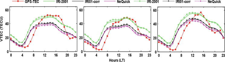
The International Reference Ionosphere (IRI) model, which was posited for application internationally by the Committee on Space Research (COSPAR) and the International Union of Radio Science, is one of the most widely used models (URSI). Its primary function is the specification of ionospheric parameters [44]. The IRI defines averages once a month of electron density, ion temperature, electron temperature, ion composition, and ion drift at heights ranging between 60 km and 1500 km for given times, dates, and locations. The development of this model is still in progress. The IRI’s capacity for determining and predicting ionospheric behavior is continuously updated by the scientific community. The current version of the IRI is the IRI-2016 model, which was released with several modifications [45]. The IRI-2016 model has three topside electron density options, namely IRI-2001, IRI01-corr, and NeQuick. Various topside electron density options are expressed by various mathematical functions. The electron density profile with the NeQuick and IRI01-corr topside options decreases with altitude more swiftly than that with the IRI-2001 topside option [46]. Many researchers worldwide have compared these different topside electron density options to identify the best option and tested the latest IRI version in certain regions [47, 48, 49]. The performance of the latest IRI-2016 model using three topside options was compared to the IRI-2012 model at different stations on the equator. They observed that the IRI-2016 model showed some improvements in comparison with the IRI-2012 model and the IRI01-corr; however, Elmunim et al. [16] displayed a minimum error compared to the IRI-2001 and NeQuick topside options. Figure 4 depicts the hourly variation on a quiet day (7 March 2013) in an equatorial region over the UUMK, MUKH, and TGPG stations. The first row shows the variation by the hour at the UUMK, MUKH, and TGPG stations. The vertical axis represents the VTEC values (TECU), while the horizontal axis displays the hours. The topside options of the IRI-2016 are represented by a solid line, while the topside options of the IRI-2012 are represented by dotted lines, showing the IRI-2001, which is in green, IRI01-corr in black, and the NeQuick in pink. When compared to IRI-2016 and IRI-2012, the IRI01-corr and NeQuick offered better predictive ability during the day, except for the afternoon, when the IRI-2001 model provided a better result prediction. In comparison to the IRI-2001 and NeQuick options, the IRI-2016 and IRI-2012 models of the IRI01-corr option produced smaller percentage deviation values. The IRI-2016 outperformed the IRI-2012 in the IRI01-corr and NeQuick options in the majority of the daily disturbed and quiet periods.

Figure 4.

The diurnal hourly variation of IRI-2016 and IRI-2012 topside options. IRI-2016 (IRI-2001, IRI01-corr, and NeQuick) are plotted in solid lines, while IRI-2012 (IRI-2001, IRI01-corr, and NeQuick) are plotted in dotted lines.

10.2 Time series models

The time series statistical models have been developed to estimate and correct the ionospheric delay and for ionospheric forecasting. A time series is a collection of observations with equal time spacing that are measured sequentially. The observation of GNSS data, in this case, the double difference in the ionosphere between a reference and a roving satellite on a specific baseline, is a strong example of such a series. Time series are analyzed as tools for understanding the primary structure and function that created the data. Based on the understanding of these mechanisms, a time series can be mathematically modeled to forecast future observations. Therefore, some researchers have successfully developed a series of high-precision ionospheric prediction models, such as the time series models of Refs. [50, 51, 52, 53]. Among these models, the time series model has several advantages over other modeling techniques. It uses less sampling data, includes a complete modeling theory, has a relatively simple calculation process, has good extensionality, and delivers high-precision short-term ionospheric predictions [53].

In addition, the Autoregressive-Integrated Moving Average (ARIMA) method is a time series technique that was created by Box and Jenkins in 1976. This technique allows the production of a set of weighted coefficients that describe the ionosphere’s behavior or rate of change during the sample period. These coefficients can then be used to forecast future observations. Serval researchers used the model to correct the ionospheric delay in different equatorial regions [30, 54].

Additionally, the Holt-Winter approach is a statistical time series approach used to forecast future data values to generate repeated trends and a seasonal pattern time series [55]. The exponential smoothing function method is applied to reduce variations in the time series data to provide a clearer viewpoint [56]. The model has additive and multiplicative options. The multiplicative options showed better results with high accuracy compared to the additive option [57]. The model was developed toward forecasting ionospheric delays and thus enhances positional accuracy by up to 95% in equatorial regions [19].

Elmunim et al. [18] compared the empirical IRI model using IRI01-corr, IRI-2001, and NeQuick topside options with the time series statical model Holt-Winter over the Langkawi, Malaysia, station in an equatorial region. Malaysia’s geographic coordinates in daily, monthly, and seasonal variation, as well as during the geomagnetically disturbed period over the equatorial region are 6.19°N and 99.51°E. In comparison to the IRI01-corr, NeQuick, and Holt-Winter methods, the IRI-2001 had the greatest percentage deviation. Therefore, as shown in Figure 5, the model’s accuracy was discovered to be about 95% for the Holt-Winter method, 75% for the IRI01-corr, 73% for the NeQuick, and 66% for the IRI-2001 model.

Figure 5.

The accuracy of the ionospheric models in equatorial station.

The Holt-Winter method performed better and estimated the TEC more accurately than the IRI01-corr and NeQuick, whereas the IRI-2001 performed poorly in the equatorial region over Malaysia. The comparative study helps to understand the model to further improve the accuracy of the GNSS. These studies are highly beneficial in correcting ionospheric delays and providing GNSS data correction, hence assisting in future accuracy improvements of the GNSS.

11. Conclusion

The GNSS satellites transmit signals propagate through the ionosphere. Ionospheric delay is one of the main sources of error that disrupts the accuracy of the GNSS signals as it changes the propagated signal’s velocity. This delay can range from a few meters to tens of meters. Understanding the characteristics of the ionosphere and the estimation of the ionospheric delay are important when investigating the ionospheric delay and identifying an accurate model in a specific region. The model’s accuracy depends on the complexity of the ionospheric structure and the propagating frequency of the radio waves. In equatorial regions, the time series model has given highly efficient results compared to empirical models. It is important to determine the most effective model to reduce GNSS errors and improve the accuracy of the GNSS.

References

1.Jensen AB, Mitchell C. GNSS and the ionosphere. GPS World. 2011;22(2):40-42
2.Elmunim NA, Abdullah M. Ionosphere. In: Ionospheric Delay Investigation and Forecasting. Singapore: Springer; 2021. pp. 19-29
3.Okoh D. GPS Modeling of the ionosphere using computer neural networks. In: Rustamov RB, Hashimov AM, editors. Multifunctional Operation and Application of GPS. London, UK: IntechOpen; 2018. DOI: 10.5772/intechopen.75087
4.Parkinson BW, Enge PK, Spilker JJ. Differential gps. Progress in Astronautics and Aeronautics: Global Positioning System Theory and Applications. 1996;2(164):3-32
5.Khan SZ, Mohsin M, Iqbal W. On GPS spoofing of aerial platforms: A review of threats, challenges, methodologies, and future research directions. PeerJ Computer Science. 2021;7:e507. DOI: 10.7717/peerj-cs.507
6.Karaim MO, Karamat TB, Noureldin A, Tamazin M, Atia MM. Real-time cycle-slip detection and correction for land vehicle navigation using inertial aiding. In: Proceedings of the 26th International Technical Meeting of the Satellite Division of the Institute of Navigation (ION GNSS+ 2013). 2013. pp. 1290-1298
7.Van Dierendonck AJ, Hegarty C, Scales W, Ericson S. Signal specification for the future GPS civil signal at L5. In: Proceedings of the IAIN World Congress and the 56th Annual Meeting of the Institute of Navigation (2000). 2000, June. pp. 232-241
8.Betz JW. Effect of linear time-invariant distortions on RNSS code tracking accuracy. In: Proceedings of the 15th International Technical Meeting of the Satellite Division of the Institute of Navigation (ION GPS 2002). 2002. pp. 1636-1647
9.Zhang J, Lachapelle G. Precise estimation of residual tropospheric delays using a regional GPS network for real-time kinematic applications. Journal of Geodesy. 2001;75(5):255-266
10.Chen H, Li W, Liu X, Jiao W. A study on measuring channel bias in GNSS receiver. In: China Satellite Navigation Conference (CSNC) 2015 Proceedings. Berlin, Heidelberg: Springer; 2015. pp. 343-352
11.Håkansson M, Jensen AB, Horemuz M, Hedling G. Review of code and phase biases in multi-GNSS positioning. GPS Solutions. 2017;21(3):849-860
12.Mirmohammadian F, Asgari J, Verhagen S, Amiri-Simkooei A. Multi-GNSS-weighted interpolated tropospheric delay to improve long-baseline RTK positioning. Sensors. 2022;22(15):5570
13.El-Rabbany A. GPS Positioning Modes, Introduction to GPS: The Global Positioning System. Norwood. MA: Artech House. Inc; 2002. pp. 69-83
14.Guo Z, Yu X, Hu C, Jiang C, Zhu M. Research on linear combination models of BDS multi-frequency observations and their characteristics. Sustainability. 2022;14(14):8644
15.Nade DP, Potdar SS, Pawar RP. Study of equatorial plasma bubbles using ASI and GPS systems. In: Geographic Information Systems in Geospatial Intelligence. London, UK: IntechOpen; 2020
16.Elmunim NA, Abdullah M, Bahari SA. Evaluating the performance of IRI-2016 using GPS-TEC measurements over the equatorial region. Atmosphere. 2021;12(10):1243
17.Elmunim NA, Abdullah M. Ionospheric delay forecasting. In: Ionospheric Delay Investigation and Forecasting. Singapore: Springer; 2021. pp. 41-71
18.Elmunim NA, Abdullah M, Hasbi AM, Bahari SA. Comparison of GPS TEC variations with Holt-winter method and IRI-2012 over Langkawi, Malaysia. Advances in Space Research. 2017;60(2):276-285
19.Abd Elmunim N, Abdullah M, Bahari SA. Characterization of ionospheric delay and forecasting using GPS-tec over equatorial region. Annals of Geophysics. 2020;63(2):PA211
20.Antia HM, Basu S. Local helioseismology using ring diagram analysis. Astronomische Nachrichten: Astronomical Notes. 2007;328(3–4):257-263
21.Bagiya MS, Joshi HP, Iyer KN, Aggarwal M, Ravindran S, Pathan BM. TEC variations during low solar activity period (2005–2007) near the equatorial ionospheric anomaly crest region in India. In: Annales Geophysicae. Copernicus GmbH; 2009;27:1047-1057
22.Tariku YA. TEC prediction performance of the IRI-2012 model over Ethiopia during the rising phase of solar cycle 24 (2009–2011). Earth, Planets and Space. 2015;67(1):1-10
23.Shimeis A, Borries C, Amory-Mazaudier C, Fleury R, Mahrous AM, Hassan AF, et al. TEC variations along an East Euro-African chain during 5th April 2010 geomagnetic storm. Advances in Space Research. 2015;55(9):2239-2247
24.Akala AO, Somoye EO, Adewale AO, Ojutalayo EW, Karia SP, Idolor RO, et al. Comparison of GPS-TEC observations over Addis Ababa with IRI-2012 model predictions during 2010–2013. Advances in Space Research. 2015;56(8):1686-1698
25.Le Huy M, Amory-Mazaudier C, Fleury R, Bourdillon A, Lassudrie-Duchesne P, Thi LT, et al. Time variations of the total electron content in the southeast Asian equatorial ionization anomaly for the period 2006–2011. Advances in Space Research. 2014;54(3):355-368
26.Galav P, Dashora N, Sharma S, Pandey R. Characterization of low latitude GPS-TEC during very low solar activity phase. Journal of Atmospheric and Solar-Terrestrial Physics. 2010;72(17):1309-1317
27.Kumar S, Tan EL, Razul SG, See CMS, Siingh D. Validation of the IRI-2012 model with GPS-based ground observation over a low-latitude Singapore station. Earth, Planets and Space. 2014;66(1):1-10
28.Sharma SK, Singh AK, Panda SK, Ansari K. GPS derived ionospheric TEC variability with different solar indices over Saudi Arab region. Acta Astronautica. 2020;174:320-333
29.Li M, Yuan Y, Zhang X, Zha J. A multi-frequency and multi-GNSS method for the retrieval of the ionospheric TEC and intraday variability of receiver DCBs. Journal of Geodesy. 2020;94(10):1-14
30.Sivavaraprasad G, Ratnam DV. Performance evaluation of ionospheric time delay forecasting models using GPS observations at a low-latitude station. Advances in Space Research. 2017;60(2):475-490
31.Tariq MA, Shah M, Ulukavak M, Iqbal T. Comparison of TEC from GPS and IRI-2016 model over different regions of Pakistan during 2015–2017. Advances in Space Research. 2019;64(3):707-718
32.Feltens J, Angling M, Jackson-Booth N, Jakowski N, Hoque M, Hernández-Pajares M, et al. Comparative testing of four ionospheric models driven with GPS measurements. Radio Science. 2011;46(06):1-11
33.Wu X, Zhou J, Tang B, Cao Y, Fan J. Evaluation of COMPASS ionospheric grid. GPS Solutions. 2014;18(4):639-649
34.Klobuchar JA. Ionospheric time-delay algorithm for single-frequency GPS users. IEEE Transactions on Aerospace and Electronic Systems. 1987;3:325-331
35.Zhang Q, Liu Z, Hu Z, Zhou J, Zhao Q. A modified BDS Klobuchar model considering hourly estimated night-time delays. GPS Solutions. 2022;26(2):1-13
36.Angrisano A, Gaglione S, Gioia C, Massaro M, Robustelli U. Assessment of NeQuick ionospheric model for Galileo single-frequency users. Acta Geophysica. 2013;61(6):1457-1476
37.Hoque MM, Jakowski N, Orús-Pérez R. Fast ionospheric correction using Galileo Az coefficients and the NTCM model. GPS Solutions. 2019;23(2):1-12
38.Zhang X, Ma F, Ren X, Xie W, Zhu F, Li X. Evaluation of NTCM-BC and a proposed modification for single-frequency positioning. GPS Solutions. 2017;21(4):1535-1548
39.Li Z, Wang N, Wang L, Liu A, Yuan H, Zhang K. Regional ionospheric TEC modeling based on a two-layer spherical harmonic approximation for real-time single-frequency PPP. Journal of Geodesy. 2019;93(9):1659-1671
40.Ren X, Chen J, Li X, Zhang X, Freeshah M. Performance evaluation of real-time global ionospheric maps provided by different IGS analysis centers. GPS Solutions. 2019;23(4):1-17
41.Chen J, Ren X, Zhang X, Zhang J, Huang L. Assessment and validation of three ionospheric models (IRI-2016, NeQuick2, and IGS-GIM) from 2002 to 2018. Space. Weather. 2020;18(6):e2019SW002422
42.Elmunim NA, Abdullah M. Ionospheric Delay Investigation and Forecasting. Singapore: Springer; 2021
43.Böhm J, Schuh H, editors. Atmospheric Effects in Space Geodesy (Vol. 5). Berlin: Springer; 2013
44.Bilitza D, Altadill D, Zhang Y, Mertens C, Truhlik V, Richards P, et al. The international reference ionosphere 2012–a model of international collaboration. Journal of Space Weather and Space Climate. 2014;4:A07
45.Bilitza D. IRI the international standard for the ionosphere. Advances in Radio Science. 2018;16:1-11
46.Bilitza D. International reference ionosphere 2000. Radio Science. 2001;36(2):261-275
47.Mallika L, Ratnam DV, Raman S, Sivavaraprasad G. Machine learning algorithm to forecast ionospheric time delays using global navigation satellite system observations. Acta Astronautica. 2020;173:221-231
48.Pham TTH, Vu XH, Dien ND, Trang TT, Van Truong N, Thanh TD, et al. The structural transition of bimetallic Ag–Au from core/shell to alloy and SERS application. RSC Advances. 2020;10(41):24577-24594
49.Yang H, Kang SJ. Exploring the Korean adolescent empathy using the interpersonal reactivity index (IRI). Asia Pacific Education Review. 2020;21(2):339-349
50.Li W, Li F, Shum CK, Shu C, Ming F, Zhang S, et al. Assessment of contemporary Antarctic GIA models using high-precision GPS time series. Remote Sensing. 2022;14(5):1070
51.Erdoğan H, Arslan N. Identification of vertical total electron content by time series analysis. Digital Signal Processing. 2009;19(4):740-749
52.Li D, Han M, Wang J. Chaotic time series prediction based on a novel robust echo state network. IEEE Transactions on Neural Networks and Learning Systems. 2012;23(5):787-799
53.Elmunim NA, Abdullah M, Hasbi AM. Improving ionospheric forecasting using statistical method for accurate GPS positioning over Malaysia. In: 2016 International Conference on Advances in Electrical, Electronic and Systems Engineering (ICAEES). Malaysia: IEEE; 2016. pp. 352-355
54.Iyer S, Mahajan A. Short-term adaptive forecast model for TEC over equatorial low latitude region. Dynamics of Atmospheres and Oceans. 2022;2022:101347
55.Suwantragul S, Rakariyatham P, Komolmis T, Sang-In A. A modelling of ionospheric delay over Chiang Mai province. In: Proceedings of the 2003 International Symposium on Circuits and Systems. ISCAS’03. Thailand: IEEE; 2003. pp. II-II
56.Gelper S, Fried R, Croux C. Robust forecasting with exponential and Holt–Winters smoothing. Journal of Forecasting. 2010;29(3):285-300
57.Elmunim, N. A., Abdullah, M., Hasbi, A. M., & Bahari, S. A. (2015). Comparison of statistical Holt-Winter models for forecasting the ionospheric delay using GPS observations. 94.20. Cf; 91.10. Fc; 95.75. Wx.
Written By
Nouf Abd Elmunim
Submitted: 03 January 2023Reviewed: 04 January 2023Published: 08 February 2023
Open access peer-reviewed chapter