Nongravitational Accelerations: A Study on the Accelerometers of GRACE and GRACE-FO

Abstract

The nongravitational accelerations measured onboard spacecraft for the purpose of modeling the Earth’s gravitational field but also for the investigation of the upper atmosphere are crucial. This study is focused on two LEO satellites, GRACE and GRACE–FO, which carry an accelerometer that measures the nongravitational accelerations, with the most dominant being the drag and the solar radiation pressure. This study presents the physical models of the nongravitational accelerations presented in the literature for the two missions and investigates how the nongravitational acceleration measurements are affected during different time periods of the solar cycle. In addition, the effect of the penumbra transitions in the three axes of the accelerometers which present as jumps in the measurements are presented. Lastly, the response of the accelerometers is investigated during minor and major geomagnetic storms that appeared during the last two solar cycles, the 24th and the 25th.

1. Introduction

The Gravity Recovery and Climate Experiment missions (GRACE and GRACE Follow–On) are two missions whose objective is the mapping of the gravitational field of the Earth. GRACE mission launched on 17 March 2002, and for more than 15 years it was monitoring the changes of the gravity field of the Earth. GRACE-FO mission launched in 2018 is dedicated to continuing GRACE’s legacy. From the measurements of these two satellite gravity missions, apart from the mapping of the gravitational field, we are able to monitor the distribution and redistribution of the Earth’s mass and enhance our knowledge of terrestrial water storage changes, sea level changes, ice sheet and glacier mass balance, and ocean circulations [1, 2].

GRACE and GRACE-FO mission consists of a pair of satellites, named GRACE A and GRACE B for GRACE mission and GRACE C and GRACE D for GRACE-FO mission, at an altitude of $\sim 500\mathrm{km}$, on the same near-polar orbit, at a $89.5°$ inclination, with a 220-km distance separation between them. As they cross different areas of the Earth, they sense gravitational changes that are expressed as distance changes between the two spacecraft. These distance changes are measured by a microwave ranging system (K-Band) at a micrometer level of accuracy. This configuration is also referred to as a low-low satellite-to-satellite tracking (SST). Each satellite carries in addition to the microwave ranging system, a Global Positioning System (GPS) [3] that provides the absolute positions of the satellite, a high-precision accelerometer that measures the nongravitational accelerations and attitude sensors that provide measurements of the inertial orientation of the spacecraft [4].

For the accurate determination of the static global gravity field, as well as its time variability, the measurements of nongravitational accelerations are crucial [5]. From the total accelerations calculated from the second derivative of the satellites’ position measured by GPS, the nongravitational measurements are subtracted to derive the pure gravitational accelerations. Therefore, both missions carry the SuperSTAR accelerometer.

The electrostatic SuperSTAR accelerometers in both missions were manufactured by ONERA in Paris, France, and measure the nongravitational accelerations acting on each satellite such as the solar radiation pressure (SRP), the drag, the Earth radiation pressure (ERP), and the thermal radiation pressure (TRP). Its principle is that there is a proof mass fixed to center of the mass of the satellite which needs to be centered. In order to always keep the proof mass centered, voltages are applied. This control voltage defines the nongravitational forces acting on the satellite. To ensure that the accelerometer measures purely the nongravitational accelerations, its proof mass is precisely placed in the center of the mass of each satellite and the resolution is 10⁻¹⁰ m/s²$\sqrt{\mathit{Hz}}$ [6].

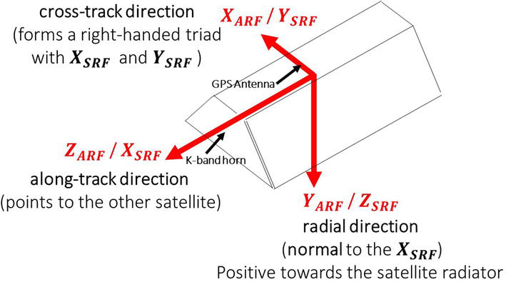
GRACE-FO accelerometers are similar to those of GRACE with some improvements to avoid temperature variation effects induced in the measurements [7]. They measure the linear and the angular nongravitational accelerations along three axes in the accelerometer reference frame (ARF) with the $Z_{\mathit{ARF}}$ defined in the along-track direction pointing toward the other satellite, $Y_{\mathit{ARF}}$ nadir-pointing and the $X_{\mathit{ARF}}$ completing the right-handed coordinate system.

The raw acceleration measurements are obtained with a sampling rate of 10 Hz (Level 1A). For the users’ convenience, the raw accelerations are filtered with a low-pass filter of 35 mHz corner frequency, time corrected, and under sampled to 1 Hz [8]. The 1-Hz accelerometer data along with most of the processed measurements are given in a dataset called Level 1b in the science reference frame (SRF), whose $X_{\mathit{SRF}}$ is pointing toward the other satellite, $Z_{\mathit{SRF}}$ is nadir-pointing, and $Y_{\mathit{SRF}}$ completes the right-handed triad [1, 4, 5]. More details on the satellite frames can be found in [9]. The satellite body-fixed reference frames are shown in Figure 1. All the original measurements that are used and will be presented in this study are derived from Level 1b data (1 Hz), of GRACE A (GRACE mission) and GRACE C (GRACE-FO mission), since GRACE A data are of a better quality than GRACE B and GRACE D accelerometer, after 1 month in orbit, presented a high signal-to-noise ratio and since then is underperforming. As a result to this malfunction, a method called transplant method is used to predict the accelerations for GRACE D, using the data of GRACE C. For more information about this method, the readers can be referred to [10, 11].

Figure 1.

The satellite body-fixed reference frames in relation to the satellite body.

As mentioned, the nongravitational accelerations acting on the satellites are the SRP, the ERP, the TRP, and the drag, with the most dominant in both missions being the SRP and the drag. Their magnitude is highly correlated with the solar cycle variations due to the solar irradiance which heats the upper atmosphere and alter the drag acting on the satellites [12]. The solar activity varies with an 11-year cycle which is defined from the cycle minima and maxima, corresponding to the increase and decrease of the sunspots [13]. GRACE mission was monitoring the Earth from 2002 until 2017, flying during the mid of solar cycle 23 and most of solar cycle 24 while GRACE-FO monitors the Earth since 2018, during the end of solar cycle 24 and the beginning of solar cycle 25. Solar cycle 23 lasted from January 1996 to December 2008 and was magnetically weak [14]. Solar cycle 24 started in December 2008 and ended in December 2019 and had an extended period of a very low sun activity. In fact, solar cycle 24 has been the weakest cycle of the past century, contrastingly to the predictions [15]. The current solar cycle 25 is believed to be similar to the 24 based on observations and predictions [16]. The contribution of the solar cycle effects in the modeling of the nongravitational accelerations will be examined in Section 2.

The modeling of the nongravitational accelerations is crucial for the prediction of a satellite’s lifetime, the thermospheric density determination, and the calibration of the accelerometer because the instrument cannot be calibrated on the ground due to strong gravitational signal. For the study of the ionosphere, the accelerometer measurements can be used in the modeling process, to determine the accuracy of the physical models but also to derive the thermospheric densities in the upper atmosphere [17, 18]. Many researchers have proposed different physical models which will be presented in Section 2, with the drag model being the one with the highest uncertainty due to its sensitivity, among others to the solar activity level.

In addition to the physical models that have been proposed for the two missions, an alternative approach to the modeling of the sum of the nongravitational accelerations is presented in this chapter. This new approach is based on the least squares spectral analysis (LSSA), and it can be used for the modeling of the sum of the SRP and the drag acting on the satellite since both forces have a period very close to the period of the satellite. After the modeling of the SRP and the drag, the residual series will be investigated for four severe geomagnetic storms during the operational years of the two missions. The investigation of the residual series of the accelerometer measurements during these storms could enhance our knowledge on how the accelerometer response changes during a geomagnetic storm, the time that the satellite measures the disturbances and their latitudinal signatures. These disturbances on the accelerometer measurements could be used in further studies as an indicator, concurrently with other magnetic and electric field measurements, of how a satellite is affected during a geomagnetic event.

2. Study of the nongravitational accelerations of GRACE and GRACE-FO

In this section, the accelerometer Level 1B data for GRACE A (GRACE mission) and GRACE C (GRACE-FO mission) satellites are presented and compared. Furthermore, the modeling of the sum of the nongravitational accelerations using the least squares spectral analysis is presented, and the residuals series during five severe geomagnetic storms are investigated.

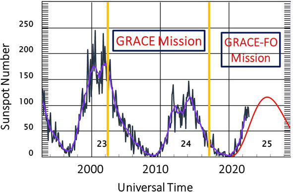
In Figure 2, the solar cycle variations are displayed with respect to the sunspot number and the operational years of the two missions. The solar cycle variations are helpful to understand the behavior of the accelerometers but also for the accuracy of the proposed physical models that have been presented for the two missions [19].

Figure 2.

Sunspot number during the operational years of GRACE and GRACE-FO mission. GRACE mission covered the declining phase of the solar cycle 23 and most of the solar cycle 24, while GRACE-FO mission was launched in the declining phase of the solar cycle 24 and is expected to cover the increasing activity of the solar cycle 25. The plotted data are available from the National Oceanic and Atmospheric Administration (NOAA).

2.1 Solar radiation pressure

The SRP accelerations are derived by the nonconservative force acting on the satellite which is produced by the impact of sunlight photons on the surface of the spacecraft. Its modeling is very important because it is one of the two dominant nongravitational forces acting on a satellite. Its magnitude depends on the reflectivity properties of the surface of the satellite, the area of the illuminated surface, the Sun-to-satellite direction, and the mass of the satellite [20]. The SRP effect on actual satellites was calculated for the first time by Parkinson, Jones, and Sapiro in 1960. Ferraz Mello [21] introduced the shadow function ψ which is actually an on-off “switch,” and it equals 1 when the satellite is illuminated by the Sun and equals 0 when the satellite is in the shadow. Sehnal [22] addressed the physical and mathematical difficulties in the modeling of the radiation pressure and introduced a special shadow function to describe the effects when the satellite enters and exits the Earth’s shadow. In the updated shadow models, the light diffusion due to the refraction, the atmospheric absorption, the effect of ozone, the relative position of the Sun, Earth, and the satellite, and the shape of the conical shadow surface have been considered.

The most commonly used SRP model is the cannonball model which assumes that the satellite’s orientation is constant with respect to the Sun. For GRACE mission, a state-of-the-art panel model has been developed that uses the optical properties of the surfaces [23].

2.2 Atmospheric drag

The atmospheric drag force is co-linear to the satellite velocity but in the opposite direction. It arises from the collisions between the satellite and the neutral and charged particles and is the main cause of the deceleration of the satellites and the decrease of their lifetime. The first scientists presented how collisions with neutral and charged particles affect the satellite orbit were Jastrow and Pearse [24]. The modulus of the atmospheric drag is commonly represented with the formula:

$$a_{\mathit{\text{drag}}}=-\frac{1}{2}\rho \frac{c_{D}A}{m}{\upsilon }_{\mathit{rel}}^2\frac{{\upsilon }_{\mathit{rel}}}{\left|{\upsilon }_{\mathit{rel}}\right|},$$E1

where $m$ is the mass of the satellite, $A$ is the area of the satellite, $c_D$ is the drag coefficient, $\rho$ is the atmospheric density, and ${\upsilon }_{\mathit{rel}}$ is the satellite’s velocity relative to the rotating atmosphere. The atmospheric density due to uncertainties caused by different solar activities and the disturbance in the magnetosphere is very difficult to model precisely. Also, the drag coefficient approximation is accurate only when the density and the velocity do not vary much along the satellite’s orbit. Lastly, one of the most important variables in the drag determination is the relative velocity which is accurate only during the assumption that the lower part of the atmosphere rotates with the Earth—an assumption that is not truly accurate with the presence of the neutral winds, which can have high velocity and affect dramatically the drag estimation.

For the drag modeling and for the understanding of the solar activity, indices such as $F_{10.7}$, $A_p,K_p$ are used. One excellent indicator of solar activity is the $F_{10.7}$ radio flux, is measured in solar flux units, and can be measured on a daily basis from the Earth’s surface. The $A_p$index provides a daily average level of the geomagnetic activity from eight daily values [25], while $K_p$ is a 3-hour average quasi-logarithmic index derived from the maximum fluctuations of the horizontal components of Earth’s magnetic field. Some of the assumptions made by the scientists to create an atmospheric drag model are the following: the use of the $F_{10.7}$ is a suitable approximation for the atmospheric models and very important in the heating of the upper atmosphere; the lower atmosphere rotates with the Earth; the temperature profiles are based on basic models; the drag coefficient is correct; and all the interpolated variables and indices such as the $A_p,K_p$ do not introduce errors in the models [26].

For the models of the aerodynamic coefficients (dimensionless quantities which characterize the aerodynamic force and moment acting on the satellite), the velocity, the temperature, and the chemical and physical conditions of the satellite surface are taken into consideration. For satellites with complex shapes, the aerodynamic coefficients are calculated by dividing the body of the satellite into segments of simpler shapes and adding them together.

2.3 Earth radiation pressure

Earth radiation pressure contains the Earth’s reflected and emitted radiation. The reflected sunlight acts on the satellites and causes ERP accelerations Earth radiation models are calculated based on three main assumptions: The Earth behaves like a Lambertian sphere; the radiation is reflected or emitted; and there is global conservation of energy [27]. The Earth’s irradiance (Earth radiation power per unit area) reaches the satellite primarily in the radial direction. The amount of reflected energy that affects the satellite is influenced by local changes in the atmospheric and surface properties of the Earth. The Earth radiation pressure should not be confused with the albedo term, since albedo and emission models are extensively used for the derivation of the ERP. A strict definition of the albedo is that albedo is called the radiative flux that includes the shortwave variations, and it is a measurement of electromagnetic radiation in the visible and near-infrared spectrum [28]. Studies have shown that the Northern and Southern Hemispheres show the same amount of irradiance. Also, there is a seasonal cycle of the surface albedo which attains a maximum in boreal springtime due to the increased reflectivity of the land surfaces been covered by snow between 30°N and 60°N. The maximum of the annual cycles of the irradiance is in March, the second maximum is in October, and the minimum is between June and July [29].

A very detailed study on the modeling of the SRP and ERP for Low Earth Orbit satellites, with an application on GRACE A data, has been published by Vielberg and Kusche [30].

2.4 Review of the physical models proposed for GRACE mission

Many physical models have been proposed for the modeling of the nongravitational accelerations for GRACE mission that can been used for the studies of the upper atmosphere but also for the calibration of the instrument which is impossible to be calibrated before the launch of the satellite due to strong gravitational signal on the ground. The SRP models presented for GRACE are of high precision and almost uncorrelated with the solar activity, since the SRP is unaffected during different solar activity levels contrastingly to the drag models which increase due to the increase of the atmospheric density [31].

One common method for the modeling of the nongravitational accelerations is the satellite acceleration approach [32]. The main idea of this approach is to derive the total accelerations acting on the satellite by double numerical differentiation of the positions estimated from the GPS measurements. This approach, even though it increases the noise of the calculated total accelerations due to the double differentiation, is very accurate as the position of the satellite can be determined with a few centimeter accuracy. Subsequently, modeled gravitational accelerations are subtracted from the total accelerations to estimate the nongravitational accelerations. Bezděk proposed a physical model using the neutral thermospheric density model DTM-2000 and the zonal and seasonal models of the ERPand the shape and physical properties of the satellite. In his work, the modeled nongravitational accelerations are shown during one orbit of GRACE A ($\sim 91$minutes) on 11 August 2003 (high solar activity), and it is observed that the modeled drag is the force that affects the most the satellite in the along-track direction ($\sim 90\mathit{nm}/s^2\text{magnitude}$), the SRP affects the cross-track direction the most ($\sim 30\mathit{nm}/s^2)$, and the SRP and the albedo are dominant in the radial direction ($\sim 50$and $\sim 10\mathit{nm}/s^2$, respectively) with the drag acceleration being almost 0.

Another high-precision model has been presented for GRACE mission that is used for the calibration of the instrument [19]. In this model, the researchers implemented their model using a tool named XHPS, developed at ZARM institude, and they based their proposed model on a detailed finite element of the satellite. A finite element model is used for the calculation of the thermal radiation pressure. The physical models for nongravitational accelerations have been presented during high (March 2003) and low (February 2009) solar activity. During high solar activity, the drag in the along-track direction is $\sim 100\mathit{nm}/s^2$, while the SRP is $\sim 40\mathit{nm}/s^2$ and similar to the SRP during low solar activity contranstingly to the drag which is one order of magnitude smaller.

Along the cross-track direction, the drag is $\sim 10$ and $\sim 1\mathit{nm}/s^2$ for high and low solar activity, respectively. The SRP is $\sim 30\mathit{nm}/s^2$. In the radial direction, the SRP is $\sim 40\mathit{nm}/s^2$, the albedo $\sim 10\mathit{nm}/s^2$, and the thermal radiation $\sim 5\mathit{nm}/s^2$. There are no significant changes in the radial direction between the high and the low activity.

All the proposed physical models are based on the satellite’s geometry and surface and material properties which are given in the GRACE Product Specification Document [33]. The atmospheric drag models are either based on the DTM2013 [34] or the JB2008 [35], and the albedo model is based on CERES [36].

2.5 GRACE A data from 2004 to 2009

As mentioned in Section 1, all the data used in this study are the Level 1B data from GRACE A and GRACE D which are available for both missions at https://podaac-tools.jpl.nasa.gov/drive.

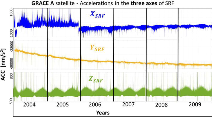
The period 2004–2009 has been chosen to depict the nongravitational accelerations as measured by GRACE-A satellite as they change during the transition from the maximum phase of the solar cycle 23 to its minimum and then to the beginning of cycle 24 (January 2009). In Figure 3, the measurements in the three axes of the Science Reference Frame (SRF) are presented.

Figure 3.

Total nongravitational accelerations along the three axes of the SRF as measured by GRACE-A in the period 2004–2009. In blue are the accelerations in the along-track direction ($X_{\mathit{SRF}}$), in yellow are the accelerations in the cross-track direction ($Y_{\mathit{SRF}}$), and in green are the accelerations in the radial direction ($Z_{\mathit{SRF}}$).

The dominant nongravitational accelerations in the $X_{\mathit{SRF}}$ are the drag and the SRP. It is clear that the amplitude of the accelerations is highly correlated with the phase of the solar cycle as it is $\sim 10\mathit{nm}/s^2$ larger when the sunspot number is $\sim 100$, and it decreases when the sunspot number approaches zero. This is due to the fact that during high solar activity, the drag acting on the satellite increases. In 2004 and 2005, the measurements show high disturbances compared to the years after 2006 due to the higher solar activity but also due to the presence of severe geomagnetic storms of a $K_p\mathit{\text{index}}=8$. There is a strong periodicity of $\sim 161$ days, which is more visible after 2006 because of the less disturbed signal. This periodicity in the accelerations is because the accelerometer is strongly correlated with the ${\beta }^{\prime }$ angle which is the angle between the satellite’s orbital plane and the geocentric position vector of the sun. This angle defines the time that the satellite spends in direct sunlight, and as it is close to $+90°$or $-90°$ the satellite is in a full sun orbit meaning that it does not enter the Earth’s shadow.

The dominant accelerations in the $Y_{\mathit{SRF}}$ are the SRP and the thermal radiation pressure (TRP) with the drag and the ERP being close to zero (less than 1 nm/s²). The cross-track axis are the least sensitive axis, but also the noisiest due to thruster activations, especially in the equatorial region and the poles. In this axis instead of the 161-day periodicity due to the ${\beta }^{\prime }$ angle, there is a 90-day periodicity because the minimum amplitude of the accelerations is during the full sun orbit and when the sun is along the radial direction, meaning that the accelerations in the cross-track direction are zero when the accelerations in the radial direction are maximum.

The dominant accelerations in the $Z_{\mathit{SRF}}$ are the SRP, the thermal radiation pressure, and the ERP. Similarly, to the other two axes, there is the strong periodicity correlated with the ${\beta }^{\prime }$ angle.

When the satellite is in a full sun orbit, the SRP is the minimum; therefore, the magnitude of the accelerations is the lowest. During the full sun orbit, the satellite does not enter and exit the Earth’s shadow; therefore, the characteristic jumps in the measurements called penumbra transitions are not present.

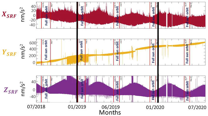
For GRACE-FO mission, GRACE C measurements are shown for the period July 2018 to July 2020. GRACE C data have been selected since the accelerometer of GRACE D is not working properly. In Figure 4, the nongravitational accelerations along the three axes are shown. GRACE C enters a full sun orbit every $\sim 158$ days compared to GRACE A which enters a full sun orbit every $\sim 161$ days. The performance of the accelerometer in GRACE C is significantly better in the$X_{\mathit{SRF}}$ than GRACE A, but the other two axes present spurious accelerations due to thruster activations.

Figure 4.

The nongravitational accelerations as measured by GRACE C from July 2018 to July 2020 in the along-track direction(red), the cross-track direction(yellow), and the radial direction (purple). The periods where the satellite is in a full sun orbit are shown with red lines.

2.6 Penumbra transitions

All satellites that carry an accelerometer on board show in their measurements perturbative effects that are caused by the penumbra transitions during their passages through the Earth’s shadow. Both GRACE and GRACE-FO accelerometer measurements are affected by the penumbra transitions on all three axes, and these measured disturbances are very useful, because they can be used to identify the passage of the satellite into the Earth’s shadow and its exit from it. This separation is very important due to the different nongravitational forces acting on the satellite during the sun segment of the orbit and the shadow segment (umbra). The importance of the eclipse transitions and their modeling was recognized by many authors that studied the effects of SRP on the motion of satellites [37, 38, 39, 40].

The accurate modeling of penumbra transitions is very challenging because it depends on the different characteristics of the satellite mission studied. Different missions due to different orbit inclination, attitude, and spacecraft shape experience different transitions, and this could cause errors in the SRP models. Therefore, misalignments in the SRP models and the estimation of the penumbra transitions between the models and the real measurements could introduce error in the calibration process of the accelerometer instrument and consequently in the extraction of gravity field models or thermospheric winds [18, 30, 41, 42]. The appearance of the transitions is correlated with the β′ angle, and the existing theoretical models present the largest deviations from the real measurements during periods of β′ angle being close to zero. During these periods, the satellite is exposed to direct sunlight for approximately half of its full orbit, and the rest of the time it passes through the Earth’s shadow, causing large temperature differences [43].

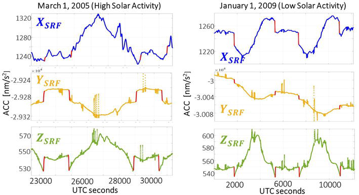
In Figure 5, the accelerometer data for GRACE A are shown. For GRACE, the penumbra transitions in the $X_{\mathit{SRF}}$ are only visible during low solar activity since the drag acting in the along-track direction is smaller than the SRP. In the other two axes, the penumbra transitions are visible throughout all the operational years.

Figure 5.

Accelerometer data of GRACE-A for two orbital revolutions on 1 March 2005(left) and on 1 January 2009 (right). The penumbra transitions appear as jumps in the measurements (indicated in red) when the satellite enters and exits the Earth’s shadow.

2.7 Modeling the total radiation pressure using least squares spectral analysis (LSSA)

The drag and the radiation pressure have dominant frequencies close to the orbital period (1 cycle per revolution) and to the semi-period (2cpr) of the satellite [4]. This allows for the modeling of the dominant nongravitational accelerations using the LSSA in the frequency domain. It is very important to note here that this analysis is based only on the measurements from the satellite, without the use of any physical model. To the best of our knowledge, this is the first study presented that models the nongravitational accelerations using the spectral characteristics of the measurements. The LSSA is used in this study to analyze both equally and unequally spaced time series contrastingly to Fourier analysis which can be used only when a time series is equally spaced and stationary [44, 45]. The software used for this analysis is in MATLAB code called LSWAVE [46] which can analyze any equally or unequally spaced time series, nonstationary or stationary. This analysis is based on the least square spectrum which provides the best measure of the power contributed by the different frequencies to the variance of the data [47]. In each trial, the least squares spectrum is calculated simultaneously for the amplitudes of all the known constituents that have been used as an input in the software. The inputs in the software are the datum shift, the linear trend, the starting time index of the penumbra transitions, the orbital frequency, and its four harmonics, and they are summarized in Table 1. After each trial, the amplitude and the phase of the sin wave of the frequencies are computed. The result after suppressing the five dominant frequencies, the datum shift, the linear trend, and the correction of the jumps in the data due to the penumbra transitions is a residual series that contains shorter drag and ERP variations.

Datum shift (refers to the mean = 0)
Linear trend
Starting time of the penumbra transitions as an index
Frequency 1 (orbital period)	0.1760 $\mathit{mHz}$
Frequency 2 (1st harmonic)	0.3525 $\mathit{mHz}$
Frequency 3 (2nd harmonic)	0.5287 $\mathit{mHz}$
Frequency 4 (3rd harmonic)	0.7004 $\mathit{mHz}$
Frequency 5 (4th harmonic)	0.8810 $\mathit{mHz}$

Table 1.

The known constituents as an input in the LSSA.

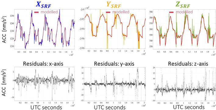
Since the modeling is based on the low-frequency components, for shorter drag variations in the along-track direction, the variations in the frequency band (0.176–0.900 $\mathit{mHz}$] have been added to the model derived from the LSSA. As it is shown in Figure 6, the residuals in the $X_{\mathit{SRF}}$ are the largest due to residual drag variations and in the $Y_{\mathit{SRF}}$ are the smallest and close to zero (the spikes in the $Y_{\mathit{SRF}}$ and $Z_{\mathit{SRF}}$ refer to the thruster activations for the attitude correction, measured by the accelerometer).

Figure 6.

Top: The original measurements from the accelerometer (Level 1b) on 1 November 2009 for the three axes (blue, yellow, and green) as measured by GRACE-A and the modeled sum of the nongravitational accelerations (red). Bottom: The residual series of the three axes.

2.8 Geomagnetic storms as observed by GRACE and GRACE-FO

After the modeling of the total nongravitational accelerations using the LSSA, the scope of this study is to investigate the behavior of the accelerometer on both missions during four severe geomagnetic storms. After the suppression of the dominant frequencies due to the drag and SRP, the residual series contain higher frequency disturbances that show the time that the satellite is affected by the geomagnetic storm, the latitudinal behavior of the disturbances, and some signature signals that could be explained as the response of the instrument due to electromagnetic disturbances. Only the disturbances in the $X_{\mathit{SRF}}$ are presented since it is the most disturbed axis during a geomagnetic storm because of the high drag variations.

Geomagnetic storms are one of the most important components for the study of the upper atmosphere and the space weather effects on Earth. They were discovered about 200 years ago, but data for their study are available the last 50 years due to satellite observations. Their investigation is very important since they can cause damage on the satellites, system failures, and navigational problems [48, 49]. Geomagnetic storms occur due to the ionization of the Earth’s atmosphere from the solar flares. The energetic particles interact with the Earth’s upper atmosphere and increase the temperature, and as a result the heating increase the drag acting on the satellites. The accelerometer data from both GRACE missions have been used for the investigation and the extraction of the thermospheric densities [50, 51, 52, 53]. Densities are used to study the response of the atmosphere to the geomagnetic activity and investigate variations in the interplanetary magnetic field (IMF), high- and low-latitude responses, hemispheric asymmetries, and variations in the solar wind pressure. In this section, the response of the accelerometer in the $X_{\mathit{SRF}}$ will be presented during four severe geomagnetic storms for GRACE and GRACE-FO. Geomagnetic Storms 8–10 November 2004.

2.8.1 Geomagnetic Storms 8-10 November 2004

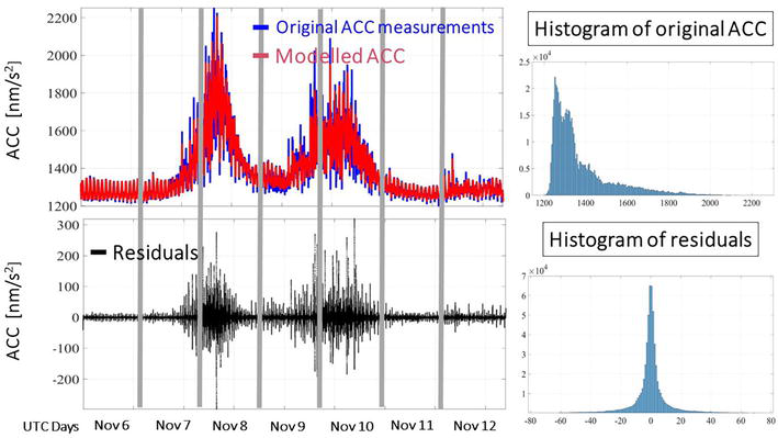
Two geomagnetic storms occurred during 8 November and 10 November 2004 due to multiple interacting coronal mass ejections (CMEs), which is something unusual during the declining phase of the 23rd solar cycle. The $D_{\mathit{st}}$ reached $-373\mathit{nT}$ during 7–8 November and $-289\mathit{nT}$ during 9–10 November. During both storms, the $K_p$ index was 9–. The first event starts occurring on 7 November around 1400–1600 UT, which reached lower latitudes at about 2300UT on the same day. The second major storm occurred after 1900 UT on 9 November and reached a peak after 0200 UT on 10 November [54, 55].

The disturbances on the accelerometer started on 7 November at 1442 UT at $70°$N with a magnitude of $\sim 28\mathit{nm}/s^2$, and the maximum disturbance occurred on 8 November at 0500 UT at $70°$N reaching a maximum magnitude of $\sim 300\mathit{nm}/s^2$. During the first event, the residual show disturbances at low latitudes at $35°$N and at mid-latitudes at $55°$S.

Between the two events, the disturbances become smaller but on 9 November 2018 around 1000 UT at $70°$N, they start become significantly larger until they reach a maximum peak at 2000 UT of $\sim 270\mathit{nm}/s^2$ at $82°$N. The second storm lasted more than the first and the disturbances on the accelerometer until 10 November at 2100 UT.

In Figure 7, the Level 1B measurements, the modeled nongravitational accelerations, and the residuals, with their histograms, are shown. The two events can be easily distinguished in both the original measurements and the residual series.

Figure 7.

Top left: The nongravitational accelerations as measured from GRACE A from 6 November to 12 November 2004 (blue) and the modeled accelerations (red). Top right: The histogram of the original measurements of GRACE A. Bottom left: The residual series resulted from the subtraction of the modeled accelerations from the accelerations of GRACE A. Bottom right: The histogram of the residual series.

2.8.2 Geomagnetic storm of 21–22 January 2005

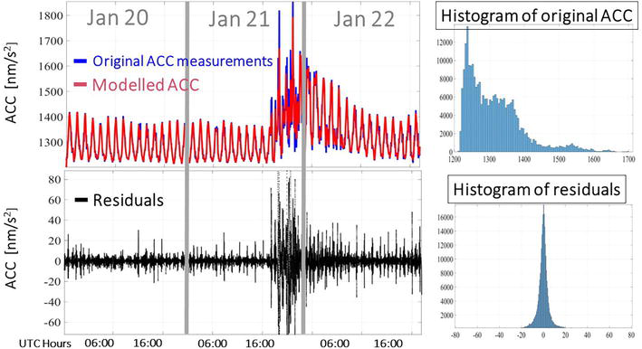
On 20 January 2005, an outstanding solar flare occurred and released a coronal mass ejection creating a geomagnetic storm of a $K_p$ index of 8. The minimum $D_{\mathit{st}}=-105\mathit{nT}$ was reached at 0600 UT on 22 January. A strong interplanetary shock created a sudden impulse (SI) at 1712 UT, causing a significant compression of the magnetosphere [56, 57].

In Figure 8, the nongravitational accelerations as measured by GRACE A during 20 January to 22 January, the modeled accelerations from the LSSA and the residuals series are displayed along with their histograms. From the measurements of the accelerometer, it is shown that the disturbances in the measurements due to the geomagnetic storm start on 21 January at 1742 UT. The higher disturbances last until 21 January at 2248 UT but are clearly from the residuals that the disturbances are also present on 22 January.

Figure 8.

Top left: Nongravitational accelerations as measured by GRACE A from 20 January 2005 to 22 January 2005 (blue) and the modeled accelerations (red). Top right: The histogram of the original nongravitational accelerations. Bottom left: The residual series after the subtraction of the modeled accelerations from the original measurements of GRACE A.

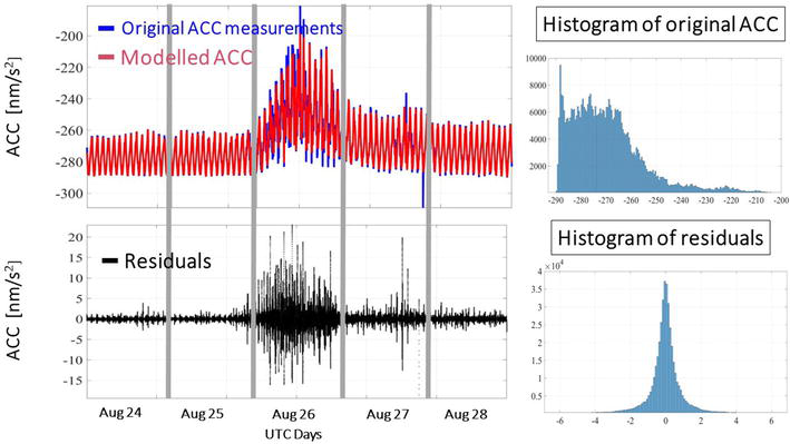
2.8.3 Geomagnetic storm of 25–26 August 2018

GRACE-FO mission is launched in 2018 at the deep minimum of a rather weak solar cycle 24. On 25–26 August 2018, a G3 class storm occurred with a $K_p$ index of 7. The CME event arrived at Earth on 25 August at 0200 UT and caused a compression on the magnetosphere at 1200 UT. At 1600 UT, a negative direction of $B_Z$ component triggered the main phase of the storm. The minimum $D_{\mathit{st}}=-175\mathit{nT}$ was reached at 0600 UT on 26 August [58, 59]. From July 2018 to December 2020, this is the only storm that reached a $K_p$ index of 7. On the residual series, in Figure 9, the disturbances started on 25 August at 2100 UTC and reached a peak of $\sim 21\mathit{nm}/s^2$ at 0800 UT on 26 August. Disturbances are also shown on 27 August, during the recovery phase of the storm. Comparing the residual series from GRACE-FO and GRACE, it can be observed that residual series on GRACE-F reach a magnitude of $\sim 21\mathit{nm}/s^2$, while for GRACE their magnitude could reach $\sim 300\mathit{nm}/s^2$. This can be attributed in the declining phase of the solar cycle 24 since as it was mentioned in Section 2.1, and the magnitude of nongravitational accelerations is highly correlated with the solar cycle variations.

Figure 9.

Top left: Nongravitational accelerations as measured by GRACE C (blue) and the total modeled nongravitational accelerations (red). Top right: The histogram of the original measurements of GRACE C. Bottom left: The residual series after the subtraction of the modeled accelerations from the measured accelerations. Bottom right: The histogram of the residual series.

The accelerometer response in both missions during a geomagnetic storm is immediate. Disturbances are visible even after the main phase of the geomagnetic storm due to minor decrease in the ${\mathit{B}}_{\mathit{Z}}$ component. The geomagnetic storm in January 2005 was the only case in our analysis where the higher disturbances were present on the Southern Hemisphere instead of the Northern Hemisphere, probably because it was the only storm triggered by a northward direction of the ${\mathit{B}}_{\mathit{Z}}$.

3. Conclusions

The purpose of this study was the analysis of the accelerometer measurements of two very important LEO missions, GRACE and GRACE-FO. The correlation between the magnitudes of the measurements with solar activity variations is presented and showed that the measurements are very sensitive to solar activity variations, as expected since they measure, among other components, the atmospheric drag which is highly sensitive to these variations. GRACE-FO measurements are of a better quality in the along-track direction than GRACE mission and of much smaller magnitude, but this could be attributed not only to the instrument performance but also to the operational years that GRACE-FO monitors the Earth (low solar activity).

A literature review of the different models that have been proposed in the modeling of nongravitational accelerations is implemented, showing that the SRP and ERP models present higher accuracy than the atmospheric drag models, which is a rather challenging task due to the complexity of the particle interactions in the upper atmosphere. An alternative method of modeling the sum of the drag and the Radiation Pressure acting on the satellite using a least squares approach is presented, which is based on the frequency domain. This method can be used for the modeling of the dominant drag and RP accelerations, since the accelerations produced by these two forces show a strong periodicity very close to the orbital period of the satellite. Shorter variations in the frequency band (0.176–0.900 $\mathrm{mHz}$) are attributed to the drag in the along-track axis, since they are very close to the orbital period and its four harmonics. The residual series in the cross-track direction are almost zero, while in the radial direction show structured signals that could be attributed to ERP variations. The along-track direction presents the largest residuals due to remaining drag accelerations in the signal.

The accelerometer response during four geomagnetic storms is investigated. Three severe storms are analyzed during GRACE mission and only one for GRACE-FO, as until December 2020 there was only one severe magnetic event. There is an immediate response in the accelerations even during the initial phase of the storm. The disturbances in the residual series last until the recovery phase, something that could be explained due to the slow recovery of the atmosphere after a severe magnetic event. During the main phase of the storms, disturbances can reach low latitudes in both hemispheres, but the highest are present in the Northern Hemisphere, except from the storm in January 2005. Please note that this study does not claim that accelerometer could measure a direct effect of a geomagnetic event on the satellite. These disturbances could have been caused due to an electrostatic coupling or because the accelerometer detects a mechanical excitation as the satellite flies in a very disturbed and hostile environment which affect its instrumentation.

This study aims to enhance the knowledge of the reader about an instrument very crucial for the studies of the upper atmosphere. Numerous studies have used the accelerometer data for the extraction of the thermospheric densities, and this is beyond the scope of this study. From a preliminary investigation of the residual series of the accelerometer during minor or severe geomagnetic storms, useful time and spatial information of the disturbances are derived and if used together with other electromagnetic field measurements could lead to a better understanding on the numerous interactions that take place in the upper atmosphere.

Acknowledgments

This research was partially supported by the Natural Science and Engineering Research Council (NSERC) of Canada and by a Lassonde School of Engineering Special Research internal grant. The data used by this research can be accessed via podaac.jpl.nasa.gov.

Conflict of interest

The authors declare no conflict of interest.