Modeling Invasive Prosopis juliflora Distribution Using the Newly Launched Ethiopian Remote Sensing Satellite-1 (ETRSS-1) in the Lower Awash River Basin, Ethiopia

Abstract

Ethiopia successfully launched its first earth-observing satellite sensor in December 2019 for the purpose to manage natural resources and enhance agriculture. This study aimed at evaluating the potential of Ethiopian Remote Sensing Satellite 1 (ETRSS-1), for the first time, for detecting and mapping Prosopis juliflora distribution. To better test its potential, a comparison was made against the novel Sentinel-2 Multispectral Instrument and Landsat-8 Operational Land Manager datasets. Radiometric indices (Scenario-1) and spectral bands (Scenario-2) derived from these sensors were used to model the distribution of Prosopis juliflora using the random forest modeling approach. A total of 241 georeferenced field data on species presence and absence data were used to train and validate datasets in both scenarios. True skill statistics (TSS), area under the curve (AUC), correlation, sensitivity, and specificity were used to evaluate their performance. Our results described that the ETRSS-1-derived variables can be sufficient for modeling and mapping of P. juliflora distribution in such settings. However, higher performance was found from Sentinel-2 with AUC > 0.97 and TSS > 0.89, and followed by Landsat-8 with AUC > 0.93 and TSS > 0.77 and ETRSS-1 with AUC > 0.81 and TSS > 0.57. The lower performance of ETRSS-1 compared to Landsat-8 and Sentinel-2 datasets, however, is partly due to its coarse spectral resolution. Hence, improving the spectral resolution of ETRSS-1 might increase its accuracy.

1. Introduction

Since the successful launch of the first satellite in 1957, Sputnik-1, satellite remote sensing has been in continuous development [1, 2]. Nowadays, several state-of-the-art sensors are on board providing multispectral and hyperspectral information. After the successful launch of Landsat-1 in July 1972, the joint National Aeronautics and Space Administration (NASA) and the United States Geological Survey (USGS) launched Landsat Thematic Mapper (TM) in 1982, Landsat Enhanced Thematic Mapper (ETM) in 1999, and Landsat Operational Land Manager (OLI) in 2013 [3]. Moreover, NASA is still under continuous development and launched Landsat-9 (OLI-2) in September 2021. In addition, the French government has successfully launched seven Satellite Pourl’ Observation de la Terre (SPOT) since its first successful launch, SPOT-1, on 22 February 1986. Moreover, the European Space Agency (ESA) Copernicus program launched a series of satellites of Sentinel-1A and 1B, Sentinel-2A and 2B, and Sentinel-3A and 3B. In addition, ESA will launch Sentinel-4, Sentinel-5, and Sentinel-6 and another 6 second-generation satellite series (Sentinel-7 to 12) in the coming years.

Though many satellite sensors are currently available onboard, these satellites are mainly launched and owned by developed nations. Due to its high investment and skilled manpower requirement, so far, only 11 African nations have successfully launched 36 satellites into orbit with the collaboration of developed nations [2]. In collaboration with the Chinese government, Ethiopia successfully launched its first (Ethiopian Remote Sensing Satellite (ETRSS-1)) satellite in December 2019. It is a sun-synchronous orbit providing information at 13.75 meters of spatial resolution every 4 days. Beside, they are multispectral imagery providing information at four different spectral bands (Blue, Green, Red, and Near-Infrared). The launch of these and other states of art earth-observing satellite sensors is believed to provide reliable information for natural resource management [4, 5].

Remotely sensed-based modeling and quantifying of invasive species distribution can benefit from remotely sensed derived radiometric indices, and/or spectral bands, and/or environmental variables and/or their combinations. The commonly used approach is the use of remotely sensed derived vegetation, soil and water indices, and biophysical variables such as normalized difference vegetation index (NDVI), soil adjusted vegetation index (SAVI), normalized difference water index (NDWI), and leaf area index (LAI). A study by Ahmed et al. [6] and Ng et al. [7] employed vegetation indices (Vis) derived from Sentinel-2 to model the distribution of invasive Prosopis juliflora (P. juliflora) in Ethiopia and Kenya, respectively. Beside, Wakie et al. [8] used VIs derived from Moderate Resolution Imaging Spectroradiometer (MODIS) to map and model the distribution of P. juliflora in Ethiopia. Moreover, detecting and mapping invasive species can also be possible using spectral bands. A study by Arogoundade et al. [9] successfully mapped the distribution of Parthenium hysterophorus invasion using Sentinel-2 Multispectral Instrument (MSI) derived VIs and spectral bands. Furthermore, several studies also employed the integration of radiometric indices, spectral bands, and topo-climatic variables for mapping invasive species distribution [9, 10, 11].

Owing to the spectral, spatial, and temporal variation of Earth Observation (EO) satellite sensors, evaluating the relative potential of models derived from varied EO datasets is highly required. Models based on the freely available Sentinel-2 MSI and Landsat-8 OLI, for example, were evaluated for different applications such as soil salinity detection [12], geological mapping [13], water hyacinth [14], and greenhouse gas detection [15]. A study by Jensen et al. [16] evaluated the potential of models derived from Sentinel-2 variables against Airborne Visible/Infrared Imaging Spectrometer (AVIRIS) hyperspectral data for mapping invasive Kudzu species distribution in the USA. Similarly, a study by Ng et al. [7] made a comparison between models derived from Sentinel-2 and Pléiades-derived for mapping invasive P. juliflora in Kenya. In addition, Alvarez-taboada et al. [17] used unmanned areal vehicle (UAV) and WorldView-2-derived variables to map invasive species distribution. Moreover, previous studies in the study area were focused on either MODIS [8], Landsat-8 OLI [18], or Sentinel-2 [6] derived variables. However, identification and mapping of invasive P. juliflora distribution using ETRSS-1 are missing. Hence, this study aims, for the first time, at evaluating the potential of the ETRSS-1-derived to map and model the distribution of invasive P. juliflora in arid and semiarid regions of Ethiopia. To better evaluate its performance, a comparison was made against Landsat-8 OLI and Sentinel-2-derived variables.

2. Materials and methods

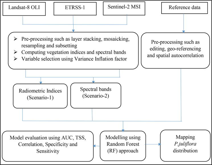
This study evaluated the relative potential of models derived from ETRSS-1 for detecting and mapping the distribution of invasive P. juliflora in the lower Awash River basin, Ethiopia. Its potential was also evaluated against Landsat-8 OLI and Sentinel-2B-derived variables. The overall process to evaluate its potential is presented in Figure 1.

Figure 1.

Methodological flow chart describing the overall process of modelling P. juliflora distribution using sentinel-2B level 2A, ETRSS-1, and Landsat-8 OLI-derived VIs and spectral bands.

2.1 Study area and species

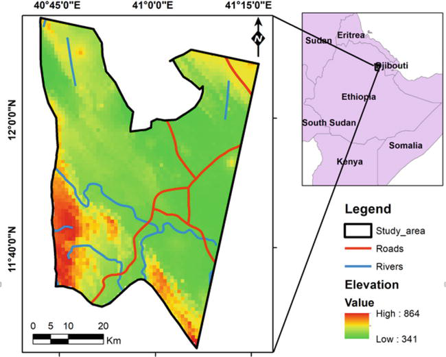
The study was carried out in the lower Awash River basin, Ethiopia, extending from 40.71° to 41.1° longitude and 11.41° to 12.26° latitude (Figure 2). It covers 3381.3 KM² ranging between 240 and 1341 meters elevation above sea level. According to the National Metrological Agency (NMA) (2020), the mean annual rainfall and temperature at Aysaita and Dubti stations were reported as 160 mm & 214 mm and 28.1°C & 29°C, respectively. Bush-shrub and woodlands (30.5%), Barelands (25.4%), Grasslands (23.9%), and P. juliflora (14.5%) are the dominant land cover in the region [19]. Furthermore, Acacia nilotica, Acacia robusta, Acacia Senegal, and Tamarix nilotica are the dominant plant species along the Awash River basin [20].

Figure 2.

Location of the study area (right) including roads, elevation, and rivers map of East Africa (right), including the location of the study area.

The Awash River basin is the most widely used river for irrigation, agriculture, hydropower, and drinking water [21]. Pastoralism and agropastoralism are the dominant sources of livelihood [22, 23]. However, environmental challenges such as regular droughts, flooding, soil erosion and salinity, overgrazing, and the spread of invasive plant species, such as P. juliflora, are the major challenges affecting land use management in the area [24]. P. juliflora was purposely introduced in the early 1980s to support soil and water management and to combat drought and conservation in the dryland parts of the country [8, 25]. However, after a few years, it becomes invasive and poses a huge negative impact on agricultural and grazing lands, native grasses, and wetlands, which are the main sources of livelihood in the region [8, 26]. As a result, the Ethiopian government declared the species as a dangerous plant that needs to be controlled, managed, and if possible removed [27].

2.2 Data

2.2.1 Reference data

For modeling the current distribution of P. juliflora, georeferenced survey data on its occurrence and absence points were collected with the help of the Global Positioning System (GPS) from January to February 2020. A stratified random sampling approach was used and 241 points were collected. Out of which, 30% were occurrences, while 70% were absence points. This share was chosen considering the previous distribution of P. juliflora in the area [18, 28]. Moran’s Index was used to assess the spatial autocorrelation among observations. As a result, we found a Moran’s Index of 0.28 and a Z-score of 2.45, suggesting no apparent spatial clustering among the points [29]. Furthermore, 70% and 30% of the collected data were used to train and test models, respectively [30].

2.2.2 Satellite data acquisition and processing

In this study, ETRSS-1 level-2B, Sentinel-2B level-2A, and Landsat-8 OLI level-2 were used. Detailed descriptions of satellite acquisition dates and their spatial characteristics are presented in Tables 1 and 2. Sentinel-2B level-2A dataset was acquired from European Space Agency (ESA) (https://scihub.copernicus.eu/dhus/#/home). It provides geometric and radiometrically corrected images. It also provides the bottom of the atmosphere (BOA) reflectance image converted from the level-1C top-of-atmosphere [31]. In addition, Landsat-8 OLI was acquired from the United States Geological Survey (USGS) (https://earthexplorer.usgs.gov/). Furthermore, Level-2B, ETRSS-1 acquired from the Ethiopian Space Science Technology Institute, Department of remote sensing development and research. Moreover, the radiometric calibration and atmospheric correction for both Landsat-8 OLI and ETRSS-1 were conducted using the FLAASH module in ENVI 5.3.

Satellite sensors	Date of acquisitions	Spatial resolutions in meter
ETRSS-1	08/03/2020	13.75
Landsat-8 OLI	29/02/2020 to 19/01/2020	30
Sentinel-2	19/01/2020 to 28/02/2020	10-20

Table 1.

Date of acquisitions and spatial resolutions of satellite sensors.

ETRSS-1 Landsat-8 OLI Sentinel-2
Spectral bands	WLR (μm)	Spectral bands	WLR (μm)	Spectral bands	WLR (μm)
B1-B	0.45–0.52	B2-B	0.45–0.51	B2-B	0.458–0.523
B2-G	0.52–0.59	B3-G	0.53–0.59	B3-G	0.543–0.578
B3-R	0.63–0.69	B4-R	0.64–0.67	B4-R	0.650–0.680
—	—	—	—	B5-RE1	0.698–0.713
—	—	—	—	B6-RE2	0.733–0.748
—	—	—	—	B7-RE3	0.773–0.793
B4-NIR	0.77–0.89	—	—	B8-NIR	0.785–0.900
		B5-NIR	0.85–0.88	B8A-NNIR	0.855–0.875
		B6-SWIR1	1.57–1.65	B11-SWIR1	1.565–1.655
		B7-SWIR2	2.11–2.29	B12-SWIR2	2.1–2.28

Table 2.

Spectral bands and their wavelength range of satellite sensors used in the study.

Where WLR is wave length range, B is blue, G is green, R is red, NIR is near-infrared, SWIR is short wave infrared, RE is a red edge, and NNIR is narrow near-infrared.

A total of four Sentinel-2B, three ETRSS-1, and two Landsat-8 OLI scenes were required to cover the study area. Bilinear interpolation was used to resample Sentinel-2B 20 M to 10 M pixel spacing. Pre-processing such as layer stacking, image mosaicking, and sub-setting for these scenes were processed using Sentinel Application (SNAP) 7.0, ENVI 5.3, and ArcGIS 10.8 software.

3. Methods

To evaluate the potential of ETRSS-1in modeling invasive P. juliflora distribution, two model scenarios were developed. The first scenario considers spectral bands derived from ETRSS-1 level-2B, Sentinel-2B Level-2A, and Landsat-8 level-2. Four bands of ETRSS-1, 10 bands of Sentinel-2B, and six bands of Landsat-8 were used. However, the three “atmospheric bands” (Band 1, 9, and 10) from Sentinel-2B level-2A and two “radar bands” (Bands 10 and 11), cirrus (band 9), and coastal aerosol (band 1) from Landsat-8 OLI level-2 were excluded from this study (Table 2).

The second scenario examines radiometric indices derived from the above three satellite datasets. Radiometric indices are a quantifiable measurement of a property that is produced by combining multiple spectral bands and which would not otherwise be apparent if only one band were used. Thirty commonly used radiometric indices were collected from the study of Ahmed et al. [6] and Ng et al. [7]. Twenty strongly collinear variables were excluded and 10 variables (Table 3) were maintained using the VIF correlation method with threshold values less than 0.9 [30, 32] in the R 4.0 software (R Development Core Team, 2021) “sdm” package [33]. This process was repeated for different sensors, and the common variables in all sensors (10 variables) with threshold values less than 0.9 were consistently used for different models.

Radiometric indices	Description	Formula
ARVI	Atmospherically resistant vegetation index	ARVI = (IR_factor * near_IR − rb)/(IR_factor * near_IR + rb), where: rb = (red_factor * red) − gamma * (blue factor * blue − red_factor * red), with gamma = 1. Where IR = Infrared
BI2	The second brightness index	BI2 = sqrt(((red_factor * red * red_factor * red) + (green_factor * green * green_factor * green) + (IR_factor * near_IR * IR_factor * near_IR))/3) where sqrt = square root
CI	The Color Index	CI = (red_factor * red − green_factor * green)/(red_factor * red + green_factor * green)
GNDVI	Green normalized difference vegetation index	GNDVI = (IR_factor * near_IR − green_factor * green)/(IR_factor * near_IR + green_factor * green)
MSAVI2	The second modified soil adjusted vegetation index	MSAVI2 = (1/2) * (2 * IR_factor * near_IR + 1 − sqrt((2 * IR_factor * near_IR + 1) * (2 * IR_factor * near_IR + 1) − 8 * (IR_factor * near_IR - red_factor * red)))
PSSRa	The pigment specific simple ratio	PSSRa = (IR_factor * near_IR)/(red_factor * red)
RI	Redness index	RI = (red_factor * red * red_factor * red)/(green_factor * green * green_factor * green * green_factor * green)
TNDVI	Transformed normalized difference vegetation index	TNDVI = sqrt((IR_factor * near_IR − red_factor * red)/(IR_factor * near_IR + red_factor * red) + 0.5)
TSAVI	Transformed soil adjusted vegetation index	TSAVI = s * (IR_factor * near_IR − s * red_factor * red − a)/(s * IR_factor * near_IR + red_factor * red − a * s + X * (1 + s * s)) Where: a is the soil line intercept, − s is the soil line slope, X is the adjustment factor to minimize soil noise.
WDVI	The weighted difference vegetation index	WDVI = (IR_factor * near_IR − g * red_factor * red). Where: g is the slope of the soil line.

Table 3.

Radiometric indices derived from ETRSS-1, sentinel-2B level-2A, and Landsat-8 OLI used in this study. The different bands described in the formula for different sensors are presented in Table 2.

The atmospherically resistant vegetation index algorithm (ARVI) describes its resistance to atmospheric effects and is accomplished by a self-correction process for the atmospheric effect on the red channel. This is done using the difference in the radiance between the blue and the red channels to correct the radiance in the red channel. The second brightness index (BI2) algorithm is representing the average brightness of a satellite image. The result looks like a panchromatic image with the same resolution as the original image. The color index (CI) is used for diachronic analyses and helps for a better understanding of the evolution of soil surfaces. The green normalized difference vegetation index (GNDVI) is used to identify different concentration rates of chlorophyll, which is highly correlated with nitrogen. The second modified soil adjusted vegetation index (MSAVI2) is an index created to replace NDVI when its accuracy is compromised by a lack of vegetation or chlorophyll in the plants. There is a great deal of bare soil between the seedlings, while they are in germination and leaf growth stages. The pigment specific simple ratio (PSSRa) investigates the potential of a range of spectral approaches for quantifying pigments at the scale of the whole plant canopy. The redness index (RI) is a type of soil radiometric index that is used to identify soil color variations. The transformed normalized difference vegetation index (TNDVI) algorithm indicates a relation between the amounts of green biomass that is found in a pixel. The transformed soil adjusted vegetation index algorithm (TSAVI) assumes that the soil line has an arbitrary slope and intercept, and it makes use of these values to adjust the vegetation index. The weighted difference vegetation index (WDVI) is very sensitive to atmospheric variations. It provides a good adjustment for soil background when calculating the LAI of green vegetation.

3.1 Species distribution modeling and evaluation

Random forest (RF) approach was used to model the performance of all datasets in both scenarios. The robust RF approach received increasing interest owing to its high classification and prediction accuracy, and its ability to determine variable importance [34]. Moreover, its ability to provide out-of-bag errors helps for accurate predictions of invasive species [16]. The out-of-bag errors are also considered as internal validation of the dataset for each tree [35]. Several studies described the higher performance of the RF modeling approach compared to other models [6, 18, 36, 37]. Owing to this, the robust RF [38] is the most widely used machine learning algorithm in many remote sensing-based studies [7, 16, 34, 39, 40, 41, 42, 43, 44, 45]. Its ability to efficiently run large datasets and handle high data dimensionality also makes it preferable for remote sensing-based prediction [34]. Beside, the model can be efficiently used to select variables calculated from single or several sensors [46].

The 10-fold cross-validation approach was employed for the validation of model scenarios of all datasets. Considering the statistical capabilities and its advantage to control data processing and visualization R Version 4.0 software [47], the “sdm” package [33] was used. The cross-validation method provides a standardized framework and high computing performance for managing predictive models. It can also reduce the risk of overfitting models [36]. It divides the reference data into 10 sub-datasets at random, with each sub-dataset accounting for 10% of the total [33].

True skill statistics (TSS), area under the curve (AUC), sensitivity, specificity, and correlation were used to assess the relative performance of models. TSS shows how well the model can distinguish between matches and mismatches between observation and prediction, whereas AUC shows how well the model can identify presence and absence classes. In addition, sensitivity refers to a model’s ability to predict occurrences where the species exist, whereas specificity refers to a model’s ability to predict absences where a species does not exist. Furthermore, correlation describes the relationship between observation (field data) and prediction of the model. The threshold is a point that separates the presence (above the threshold) and absence (below the threshold) of a particular species [36].

Moreover, receiver operating characteristic (ROC) curves were produced for all datasets in both scenarios. Furthermore, the sensitivity-specificity sum maximization approach was employed to select the best threshold. This approach yields the most reliable prediction [48, 49]. Beside, for each dataset of a particular scenario, binary (invaded and uninvaded) maps were generated. Accordingly, pixels above and below the threshold represent the presence and absence of P. juliflora distribution, respectively. Beside, maps showing P. juliflora distribution and their percent coverage were computed in ArcGIS 10.8 software. This was computed considering the threshold value of the models (presence and absence values). The point above the threshold is considered as the occurrence of the species, while the point below the threshold is considered as absence of the species. Moreover, variable importance was derived using the “getVarImp” function in the R Version 4.0 software [47], the “sdm” package [33].

4. Results

4.1 Performances of satellite datasets

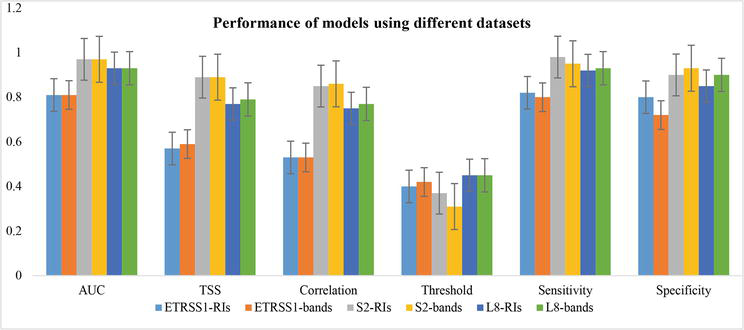
Figure 3 presented the relative performance of models derived from different satellite sensors. Accordingly, Sentinel-2-derived RIs (S2-RIs) showed higher performance with AUC = 0.97, and TSS = 0.89 followed by Landsat-8 OLI-derived RIs (L8-RIs) with AUC = 0.93 and TSS = 0.77 and ETRSS-1 RIs (ETRSS1-RIs) with AUC = 0.81 and TSS = 0.57. Furthermore, Sentinel-2 bands (S2-bands) showed higher performance with AUC = 0.97 and TSS = 0.93 followed by Landsat-8 OLI bands (L8-bands) with AUC = 0.93 and TSS = 0.79 and ETRSS1 bands (ETRSS1-bands) with AUC = 0.81 and TSS = 0.59.

Figure 3.

The relative performance of models using ETRSS-1, Sentinel-2, and Landsat-8OLI-derived RIs and spectral bands. Sensitivity and specificity describe the rate of true-positive samples and false-positive samples (errors), respectively.

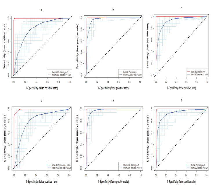
Furthermore, the receiver operator characteristics (ROC) curve (Figure 4) indicates the higher performance of Sentinel-2 (AUC > 0.97) followed by Landsat-8 OLI (AUC > 0.92) and ETRSS-1 (AUC > 0.8). ROC curve was computed using sensitivity (occurrence) and specificity (absence) values. The more the ROC curve approaches to the left the more the model becomes accurate and the more the ROC curve approaches to the diagonal line (right) the more the model needs improvement (see Figure 3).

Figure 4.

AUC using training and test datasets for (a) ETRSS1-RIs, (b) S2-RIs, (c) L8-RIs, (d) ETRSS1-bands, (e) S2-bands, and (f) L8-bands.

4.2 Variable importance

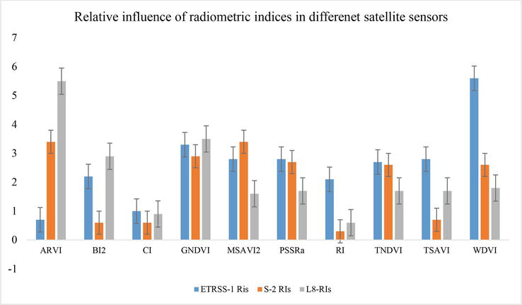
Figure 5 described the relative influence of radiometric indices for all datasets. Accordingly, WDVI, GNDVI, and TSAVI from ETRSS1-RIs, MSAVI2, ARVI, and GNDVI from S2-RIs, ARVI, GNDVI, and BI2 from L8-RIs showed higher relative importance among the radiometric indices. In addition, blue, NIR, and green bands from ETRSS-1, blue, red, and NIR bands from Sentinel-2, and NIR, red, and green bands from Landsat-8 OLI showed higher relative influence compared to the other used spectral bands. In opposite, ARVI and CI from ETRSS1-RIs, BI2, RI, and CI from S2-RIs and CI and RI from L8-RIs showed lower relative performance indicating avoiding them and/or substituting with other variables will increase the accuracy of the model. In addition, NDVI, TNDVI, and PSSRa showed comparable performance for all datasets indicating using of them will better increase the accuracy of the model.

Figure 5.

The relative influence of models using ETRSS1-RIs, S2-RIs, and L8-RIs derived variables.

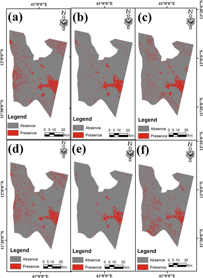
4.3 Distribution maps

Table 4 and Figure 6 described the share of invasive P. juliflora distribution using radiometric indices and spectral bands for all datasets. Accordingly, the relative distribution of P. juliflora ranges from 4.3% of S2-bands to 10.8% of ETRSS1-RIs. In addition, the ETRSS1-RIs, ETRSS1-bands, and L8-RIs identified higher P. juliflora distribution compared to the other datasets.

Datasets	Absence (%)	Presence (%)
ETRSS1-RIs	89.2	10.8
ETRSS1-bands	90.6	9.4
S2-RIs	94.1	5.9
S2-bands	95.7	4.3
L8-RIs	91.4	8.6
L8-bands	92.1	7.9

Table 4.

Proportion of P. juliflora invaded and uninvaded areas using vegetation indices and spectral bands of all datasets.

Figure 6.

P. juliflora distribution maps using different SDMs: (a) ETRSS1-RIs, (b) S2-RIs, (c) L8-RIs, (d) ETRSS1-bands, (e) S2-bands, and (f) L8-bands.

5. Discussion

Our study was intended to evaluate the potential of the newly launched satellite sensor, ETRSS-1, for detecting and mapping invasive P. juliflora distribution in the arid and semiarid regions of Ethiopia. To better evaluate its potential, a comparison was made with novel Landsat-8 OLI and Sentinel-2-derived variables. We employed both spectral bands and radiometric indices derived from each sensor. Accordingly, S2-RIs better performed with an AUC of 0.97 compared to Landsat-8 bands (AUC = 0.9) and ETRSS1-RIs (AUC = 0.83). Though its performance is lower than Sentinel-2 and Landsat-8 derived variables, ETRSS-1-derived variables showed average performance and can be sufficient for such kinds of studies. In both scenarios ETRSS-1-derived variables with AUC scores greater than 0.8 can be grouped in the category of “good” [50]. However, the capability of Sentinel-2 Landsat-8-based modeling was in the category of “excellent” as they scores greater than 0.9 of AUC.

Similar to our study, several studies described the higher performance of Sentinel-2-derived variables over Landsat-8-derived variables in the modeling of invasive species [14, 51]. Thamaga and Dube [14] tested the performance of Sentinel-2 and Landsat-8 derived RIs and spectral bands for mapping and modeling invasive Waterhyathinth and described the higher performance of Sentinel-2-derived variables. In addition, Dube et al. [51] evaluated the capability of Sentinel-2 and Landsat-8 spectral bands and vegetation indices for detecting and mapping invasive Lantana Camara and highlighted the higher accuracy of Sentinel-2 datasets. Owing to its higher spatial and spectral resolution, Sentinel-2 allows accurate identification and mapping of the fractional cover of invasive species [7, 14, 52]. Furthermore, the spectral features of four red-edge and three short wave infrared (SWIR) bands offer tremendous capacity for detecting and mapping species-level classification [16, 41, 53].

Our study also outlined the most important variables (spectral bands and radiometric indices) for detecting and mapping invasive P. juliflora distribution. Accordingly, WDVI, GNDVI, and TSAVI from ETRSS-1, MSAVI2, ARVI, and GNDVI from Sentinel-2 and ARVI, GNDVI, and BI2 from Landsat-8 showed higher relative contribution. The higher importance of vegetation indices, such as WDVI, NDVI, and TNDVI, are reported for mapping and modeling of invasive P. juliflora distribution to the study finding of Ahmed et al. [6] and Ng et al. [7]. In addition, B1 (blue) and B4 (NIR) from ETRSS-1, B2 (blue), B4 (red), and B8 (NIR) from Sentinel-2 and B5 (NIR) and B4 (red) from Landsat-8 provides higher relative contribution for modeling P. juliflora distribution. Our study is consistent with the study findings of Hoshino et al. [54], Mureriwa et al. [55], and Ng et al. [7]. A study by Ng et al. [7] described the higher importance of IR, blue, and green bands for detecting and mapping P. juliflora in Kenya. In addition, Mureriwa et al. [55] noted that P. juliflora is highly distinctive at NIR and narrow near-infrared bands. Moreover, P. juliflora showed high near-infrared and low reflectance at red bands [54].

Furthermore, comparable results between spectral bands and vegetation indices were found in all datasets indicating either spectral bands and/or radiometric indices can be applied for accurate identification and mapping of invasive species distribution. This finding is consistent with the study findings of Arogoundade et al. [9], Thamaga and Dube [14], and Dube et al. [51]. Thamaga and Dube [14] found comparable results between Landsat-8 VIs (accuracy = 65.53%) and spectral bands (accuracy = 63.34%) and Sentinel-2 VIs (accuracy = 73.31%) and spectral bands (accuracy = 73%) for mapping water hyacinth, South Africa. Our study also highlighted the higher impacts of spectral resolution on the accuracy of prediction. For example, the higher spatial resolution of ETRSS-1 (13.75 m) showed lower performance compared to Landsat-8 OLI (30 m) in both scenarios. This difference might occur partly due to their difference in spectral resolution.

6. Conclusion

In this study, we tested the potential of ETRSS-1 for detecting and mapping invasive P. juliflora distribution in the Afar regional state, Ethiopia. In addition, attempts were made to compare with Sentinel-2 and Landsat-8 OLI-derived variables. Radiometric indices (scenario-1) and spectral bands (scenario-2) were used for each dataset. Though it showed relatively lower performance, ETRSS-1 can be sufficient for mapping and identifying P. juliflora distribution. The lower performance of ETRSS-1 compared to Sentinel-2 and Landsat-8 might occur due to its coarse spectral resolution. Hence, increasing its spectral resolution with the help of different data fusion techniques might increase its accuracy.

Moreover, comparable results between spectral bands and radiometric indices were found in all datasets. This might indicate employing either spectral bands and/or radiometric indices can provide accurate identification and mapping of invasive species distribution. Accordingly, WDVI, MSAVI2, ARVI, and MNDVI from radiometric indices and B4 and B3 from spectral indices showed higher relative importance for detecting and mapping P. juliflora distribution. However, future works, such as web-based data accessibility and description of the ETRSS-1 dataset, are highly required.

Acknowledgments

This paper is part of the doctoral study entitled “Role of remote sensing in invasive species distribution modeling, the case of Prosopis in the lower Awash River basin, Ethiopia.” We would like to thank the Ethiopian Space Science and Technology Institute (ESSTI) and Wollo University for allowing this doctoral study.

Funding

None.

Author contributions

All authors contributed to the study conception and design. All authors read and approved the final manuscript.

Competing interests

The authors declare that there is no conflict of interest.

Availability of data and materials

The datasets used and analyzed during the current study are available from the corresponding author.

References

1.Tatem AJ, Goetz SJ, Hay SI. Fifty years of earth observation satellites: Views from above have lead to countless advances on the ground in both scientific knowledge and daily life. American Scientist. 2008;96(5):390-398. DOI: 10.1511/2008.74.390.Fifty
2.Woldai T. The status of earth observation (EO) & geo-information sciences in Africa – Trends and challenges. Geo-Spatial Information Science. 2020;23(1):107-123
3.Chastain R, Housman I, Goldstein J, Finco M, Tenneson K. Empirical cross-sensor comparison of sentinel-2A and 2B MSI, Landsat-8 OLI, and Landsat-7 ETM + top of atmosphere spectral characteristics over the conterminous United States. Remote Sensing of Environment. 2019;221(2019):274-285. DOI: 10.1016/j.rse.2018.11.012
4.Peerbhay K, Mutanga O, Ismail R. The identification and remote detection of alien invasive plants in commercial forests: An overview. South African Journal of Geomatics. 2016;5(1):49-67
5.Royimani L, Mutanga O, Odindi J, Dube T. Advancements in satellite remote sensing for mapping and monitoring of alien invasive plant species (AIPs). Physics and Chemistry of the Earth. 2018;112:237-245. DOI: 10.1016/j.pce.2018.12.004
6.Ahmed N, Atzberger C, Zewdie W. Species distribution modelling performance and its implication for Sentinel-2-based prediction of invasive Prosopis juliflora in lower Awash River basin, Ethiopia. Ecological Processes. 2021;10(18):1-16
7.Ng W-T, Rima P, Einzmann K, Immitzer M, Atzberger C, Eckert S. Assessing the potential of sentinel-2 and pléiades data for the detection of prosopis and vachellia spp. In Kenya. Remote Sensing. 2017;9(74):1-29. DOI: 10.3390/rs9010074
8.Wakie TT, Evangelista PH, Jarnevich CS, Laituri M. Mapping current and potential distribution of non-native Prosopis juliflorain in the Afar region of Ethiopia. PLoS One. 2014;9(11):e112854. DOI: 10.1371/journal.pone.0112854
9.Arogoundade AM, Odindi J, Mutanga O. Modeling Parthenium hysterophorus invasion in KwaZulu-Natal province using remotely sensed data and environmental variables. Geocarto International. 2019;35:13:1-15. DOI: 10.1080/10106049.2019.1581268
10.Rembold F, Leonardi U, Ng W-T, Gadain H, Meroni M, Atzberger C. Mapping areas invaded by Prosopis juliflora in Somaliland on Landsat 8 imagery. Remote Sensing for Agriculture, Ecosystems, and Hydrology XVII. 2015;9637(963723-1):295-306
11.Shiferaw H, Schaffner U, Bewket W, Alamirew T, Zeleke G, Teketay D, et al. Modeling the current fractional cover of an invasive alien plant and drivers of its invasion in a dryland ecosystem. Scientific Reports. 2019a;9(1576):1-12
12.Davis E, Wang C, Dow K, Davis E, Wang C. Comparing Sentinel-2 MSI and Landsat 8 OLI in soil salinity detection: A case study of agricultural lands in coastal North Carolina detection: A case study of agricultural lands in coastal north. International Journal of Remote Sensing. 2019;00(00):1-20. DOI: 10.1080/01431161.2019.1587205
13.Costa S, Santos V, Melo D. Evaluation of Landsat 8 and sentinel - 2A data on the correlation between geological mapping and NDVI. Geoscience and Remote Sensing. 2017;2017:1-4
14.Thamaga KH, Dube T. Testing two methods for mapping water hyacinth (Eichhornia crassipes) in the Greater Letaba river system, South Africa: Discrimination and mapping potential of the polar-orbiting Sentinel-2 MSI and Landsat 8 OLI sensors. International Journal of Remote Sensing. 2018;39(22):8041-8059
15.Novelli A, Aguilar MA, Nemmaoui A, Aguilar FJ. Performance evaluation of object-based greenhouse detection from Sentinel-2 MSI and Landsat 8 OLI data: A case study from Almería (Spain). International Journal of Applied Earth Observations and Geoinformation. 2016;52:403-411. DOI: 10.1016/j.jag.2016.07.011
16.Jensen T, Hass FS, Akbar MS, Petersen PH, Arsanjani JJ. Employing machine learning for detection of invasive species using sentinel-2 and aviris data: The case of kudzu in the United States. Sustainability. 2020;12(9):1-16. DOI: 10.3390/SU12093544
17.Alvarez-taboada F, Paredes C, Julián-Pelaz J. Mapping of the invasive species Hakea sericea using unmanned aerial vehicle (UAV) and WorldView-2 imagery and an object-oriented approach. Remote Sensing. 2017;9(913):1-17
18.Shiferaw H, Bewket W, Alamirew T, Zeleke G, Teketay D, Bekele K, et al. Implications of land use/land cover dynamics and Prosopis invasion on ecosystem service values in Afar region, Ethiopia. Science of the Total Environment. 2019b;675:354-366. DOI: 10.1016/j.scitotenv.2019.04.220
19.Shiferaw H, Bewket W, Eckert S. Performances of machine learning algorithms for mapping fractional cover of an invasive plant species in a dryland ecosystem. Ecology and Evolution. 2019c;9(5):2562-2574. DOI: 10.1002/ece3.4919
20.Tikssa M, Bekele T, Kelbessa E. Plant community distribution and variation along the awash river corridor in the main Ethiopian rift. African Journal of Ecology. 2009;48:21-28
21.Mulugeta S, Fedler C, Ayana M. Analysis of long-term trends of annual and seasonal rainfall in the Awash River basin, Ethiopia. Water. 2019;11(1498):1-22
22.Edossa DC, Babel MS, Gupta AD. Drought analysis in the Awash River basin, Ethiopia. Water Resources Management. 2010;24(7):1441-1460
23.Tadese MT, Kumar L, Koech R, Zemadim B. Hydro-climatic variability: A characterization and trend study of the Awash River basin, Ethiopia. Hydrology. 2019;6(35):1-19
24.ANRS. Afar National Regional State Rural Land Use and Administration Policy (Issue June). 2008. Available from: https://faolex.fao.org/docs/pdf/eth165071.pdf
25.Tilahun M, Birner R, Ilukor J. Household-level preferences for mitigation of Prosopis juliflora invasion in the Afar region of Ethiopia: A contingent valuation. Journal of Environmental Planning and Management. 2017;60(2):282-308
26.Ayanu Y, Jentsch A, Müller-Mahn D, Rettberg S, Romankiewicz C, Koellner T. Ecosystem engineer unleashed: Prosopis juliflora threatening ecosystem services? Regional Environmental Change. 2014;15(1):155-167. DOI: 10.1007/s10113-014-0616-x
27.MoLF. Federal Democratic Republic of Ethiopia Ministry of Livestock and Fisheries National Strategy on Prosopis Juliflora Management. 2017
28.Linders T, Bekele K, Schaffner U, Allan E, Alamirew T, Choge S, et al. The impact of invasive species on social-ecological systems: Relating supply and use of selected provisioning ecosystem services. Ecosystem Services. 2020;41(101055):1-14
29.Abdulhafedh A. A novel hybrid method for measuring the spatial autocorrelation of vehicular crashes: Combining Moran’s index and i statistic. Open Journal of Civil Engineering. 2017;7:208-221. DOI: 10.4236/ojce.2017.72013
30.Engler R, Waser LT, Zimmermann NE, Schaub M, Berdos S, Ginzler C, et al. Combining ensemble modeling and remote sensing for mapping individual tree species at high spatial resolution. Forest Ecology and Management. 2013;310:64-73
31.Szantoi Z, Strobl P. Copernicus Sentinel-2 Calibration and Validation. European Journal of RemoteSensing. 2019;52(1):253-255. DOI: 10.1080/22797254.2019.1582840
32.Zimmermann NE, Edwards TC, Moisen GG, Frescino TS, Blackard JA. Remote sensing-based predictors improve distribution models of rare, early successional, and broadleaf tree species in Utah. Journal of Applied Ecology. 2007;44(5):1057-1067
33.Naimi B, Araújo MB. Sdm: A reproducible and extensible R platform for species distribution modeling. Ecography. 2016;39:001-008. DOI: 10.1111/ecog.01881
34.Rodriguez-galiano VF, Ghimire B, Rogan J, Chica-olmo M, Rigol-sanchez JP. An assessment of the effectiveness of a random forest classifier for land-cover classification. ISPRS Journal of Photogrammetry and Remote Sensing. 2012;67:93-104
35.Boulesteix A, Janitza S, Kruppa J. Overview of random forest methodology and practical guidance with emphasis on computational biology and bioinformatics. WIREs Data Mining Knowl Discov. 2012;2:493-507. DOI: 10.1002/widm.1072
36.Ng WT, de Oliveira C, Silva A, Rima P, Atzberger C, Immitzer M. Ensemble approach for potential habitat mapping of invasive Prosopis spp. in Turkana, Kenya. Ecology and Evolution. 2018;8(23):1-11. DOI: 10.1002/ece3.4649
37.Schonlau M, Zou RY. The random forest algorithm for statistical learning. Stata Journal. 2020;20(1):3-29. DOI: 10.1177/1536867X20909688
38.Breiman L. Random forests. Machine Learning. 2001;45:5-32. DOI: 10.1201/9780367816377-11
39.Abdi AM. Land cover and land use classification performance of machine learning algorithms in a boreal landscape using Sentinel-2 data. GIScience and Remote Sensing. 2020;57(1):1-20. DOI: 10.1080/15481603.2019.1650447
40.Immitzer M, Neuwirth M, Böck S, Brenner H, Vuolo F, Atzberger C. Optimal input features for tree species classification in Central Europe based on multi-temporal Sentinel-2 data. Remote Sensing. 2019;11(2599):1-23
41.Immitzer M, Vuolo F, Atzberger C. First experience with Sentinel-2 data for crop and tree species classifications in Central Europe. Remote Sensing. 2016;8(166):1-27
42.Kosicki JZ. Generalized additive models and random Forest approach as effective methods for predictive species density and functional species richness. Environmental and Ecological Statistics. 2020;27:273-292. DOI: 10.1007/s10651-020-00445-5
43.Ma W, Feng Z, Cheng Z, Chen S, Wang F. Identifying forest fire driving factors and related impacts in China using random forest algorithm. Forests. 2020;11(507):1-26
44.Pal M. International journal of remote random forest classifier for remote sensing classification. International Journal of Remote Sensing. 2007;26(1):217-222
45.Sabat-Tomala A, Raczko E, Zagajewski B. Comparison of support vector machine and random forest algorithms for invasive and expansive species classification using airborne hyperspectral data. Remote Sensing. 2020;12:1-21. DOI: 10.3390/rs12030516
46.Belgiu M, Dragut L. ISPRS Journal of Photogrammetry and Remote Sensing. 2016;114:24-31
47.R Development Core Team. R A language and environment for statistical computing. R foundation for statistical computing, Vienna, Australia; 2020. Available from: https://www.r-project.org/index.html
48.Jimenez-Valverde A, Lobo JM. Threshold criteria for conversion of probability of species presence to either-or presence-absence. Acta Oecologica. 2007;31:361-369
49.Liu C, Berry PM, Dawson TP, Pearson RG. Selecting thresholds of occurrence in the prediction of species distributions. Ecography. 2005;28:385-393
50.González-Ferreras AM, Barquín J, Peñas FJ. Integration of habitat models to predict fish distributions in several watersheds of northern Spain. Journal of Applied Ichthyology. 2016;32:204-216. DOI: 10.1111/jai.13024
51.Dube T, Shoko C, Sibanda M, Madileng P, Maluleke XG, Mokwatedi VR, et al. Remote sensing of invasive Lantana camara (Verbenaceae) in semiarid savanna rangeland ecosystems of South Africa. Rangeland Ecology & Management. 2020;73(3):411-419. DOI: 10.1016/j.rama.2020.01.003
52.Laurin GV, Puletti N, Hawthorne W, Liesenberg V, Corona P, Papale D, et al. Discrimination of tropical forest types, dominant species, and mapping of functional guilds by hyperspectral and simulated multispectral Sentinel-2 data. Remote Sensing of Environment. 2016;176:163-176. DOI: 10.1016/j.rse.2016.01.017
53.Rajah P, Odindi J, Mutanga O, Kiala Z. The utility of Sentinel-2 vegetation indices (VIs) and Sentinel-1 synthetic aperture radar (SAR) for invasive alien species detection and mapping. Nature Conservation. 2019;35:41-61
54.Hoshino B, Karamalla A, Abdelbasit MA, Manayeva K, Yoda K, Suliman M, et al. Evaluating the invasion strategic of Mesquite (Prosopis juliflora) in eastern Sudan using remotely sensed technique. Journal of Arid Land Studies ICAL. 2012;4:1-5
55.Mureriwa N, Adam E, Sahu A, Tesfamichael S. Examining the spectral separability of Prosopis glandulosa from Co-existent species using field spectral measurement and guided regularized random forest. Remote Sensing. 2016;8(144):1-16
Written By
Nurhussen Ahmed and Worku Zewdie
Submitted: 15 April 2023Reviewed: 20 April 2023Published: 23 November 2023
Open access peer-reviewed chapter