Ionospheric Scintillation Models: An Inter-Comparison Study Using GNSS Data

Abstract

Existing climatological ionosphere models, for example, GISM, SCIONAV, WBMOD, and STIPEE, have known limitations that prevent their wide use. In the framework of ESA study “Radio Climatology Models of the Ionosphere: Status and Way Forward” their performance was assessed using experimental observations of ionospheric scintillation collected over the past years to evaluate their ability to properly support future missions, and eventually indicate their weaknesses for future improvements. Model limitations are more important in terms of the intensity scintillation parameter (S₄). To improve them, the COSMIC model has been fit (scaling factor and offset) to the measured data, and it became the one better predicting the intensity scintillation in a statistical sense.

1. Introduction

Ionospheric scintillations are the random intensity ($I$) and phase (σ_ϕ) fluctuations suffered by electromagnetic waves traversing the ionosphere due to irregularities of the electron content density, mostly originated by the solar activity and plasma irregularity processes. They are characterized by the amplitude (actually intensity, i.e., power) scintillation parameter (S₄) and the phase scintillation parameter (σ_ϕ):

$$S_4=\sqrt{\frac{⟨I^2⟩-{⟨I⟩}^2}{{⟨I⟩}^2}},$$E1

$${\mathrm{\sigma }}_{\mathrm{\varphi }}=\sqrt{⟨{\varphi }^2⟩-{⟨\varphi ⟩}^2},$$E2

where I is the intensity of the signal (i.e., power), $\varphi$ is the detrended phase of the signal, and $⟨.⟩$ denotes the time average.

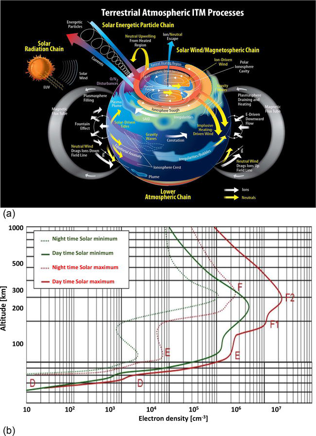
Ionospheric scintillation impacts satellite communications, global navigation satellite systems (GNSS), and remote sensors (e.g., UHF Synthetic Aperture Radars—SAR–, radar sounders, GNSS-Reflectometry, and GNSS-Radio Occultations). Ionospheric scintillation mostly occurs in equatorial and high-latitude regions, and their behavior is significantly different. The complexity of the physical processes occurring in the Earth’s ionosphere-thermosphere-mesosphere system is summarized in Figure 1a, while Figure 1b shows the main ionospheric layers and the electron density profiles during day and night.

Figure 1.

(a) Indication of the complexity of the ionosphere-thermosphere-mesosphere (ITM) system of planet Earth and the range of physical processes operating. Credits: NASA’s Goddard Space Flight Center/Mary Pat Hrybyk-Keith [https://svs.gsfc.nasa.gov/12960].(b) Typical electron density profile in the ionosphere and ionospheric layers during day/night (from https://sidstation.loudet.org/ionosphere-en.xhtml).

A summary of the main scintillation models is given in the excellent review presented in [1]:

1. Equatorial scintillations occur around ±20° of latitude of the magnetic equator, after sunset and before midnight. They are caused by small-scale structures, from tens of meters to tens of km [2], in convective plasma processes surrounding depleted ionization volumes driven through the F region, which can extend well through the F-layer peak. Irregularities with this range of scales are not independent from larger-scale plasma structures and are also related to smaller-scale irregularities.

2. Mid-latitude scintillations occur as an extension of phenomena occurring at equatorial and auroral latitudes. They can also be due to an intense sporadic E layer during daytime. High-latitude scintillations occur from the high-latitude edge of the Van Allen outer belt into the polar region. The greater scintillation occurrence is during the dark months, rather than during the months of continuous Sun illumination, at all local times.

3. Auroral zones are observed during the nighttime period. Scintillation at high latitudes is mostly refractive, and its impact in GNSS signals shows a well-known proportionality between different signal frequencies (e.g., [3]). Moreover, at high latitudes, the ionospheric disturbances mostly produce phase fluctuations, but little impact in the signal amplitude/intensity [4]. This is not the case for the low-latitude scintillation, where scintillation produces diffractive effects on the signals, and the proportionality of the effects with the signal frequency is broken and, moreover, the signal amplitude/intensity is affected (e.g., [4, 5]).

Empirical methods, such as the Basu et al. Equatorial scintillation model [6], Basu High-Latitude Scintillation Model [7], or the WAM Model [8] are restricted to geographical areas, periods of time, frequency bands in which they were derived. Analytical methods such as the Fremouw and Rino Model, the first analytical model of VHF/UHF scintillations [9], the Aarons Model [10], the Franke and Liu Model [11], the Iyer et al. Model [12], or the Retterer Model [13] assume that the ionosphere is a layer of free electrons at a given height and with a given thickness that, under the presence of the magnetic field of the Earth, disturbs the propagation of the electromagnetic waves. More recently, Liu et al. [14] and Chen et al. [15] derived an empirical model to estimate S₄ from FormoSat-3/COSMIC observations, and Kepkar et al. [16] use FormoSat-3/COSMIC data to characterize equatorial plasma bubbles.

Climatological models, include Global Climatological Models such as the WBMOD (WideBand MODel), the STIPEE, the GISM (Global Ionospheric Scintillation Model), and the SCIONAV model.¹

• WBMOD [17, 18, 19] is a climatological model for ionospheric turbulence that includes the global distribution of the electron density irregularities and the phase screen propagation model by Rino [20, 21] to calculate the effects that density irregularities produce in the propagation of electromagnetic waves. WBMOD provides modeling of the integrated strength of inhomogeneity (C_kL), the medium velocity, the anisotropy, the slope (p), and the outer scale of turbulence. Its outputs are the phase scintillation spectrum spectral index, the spectral strength parameter (at 1 Hz) T, the intensity scintillation index S₄ (Eq. (1)), and the rms of detrended phases σ_ϕ [in radians] (Eq. (2)). Assuming that the power spectral density of the phase fluctuations is isotropic, it can be approximated by:

$${\gamma }_{\varphi }\left(k\right)=\frac{C_s}{{\left(k^2+q_0^2\right)}^{p/2}},$$E3

where C_S characterizes the turbulence strength, k is the wave number, q₀ = 2π/L₀ being L₀ the outer scale of the inhomogeneities, and p is the spectrum slope (the spectrum is linear in log–log scale).

WBMOD gives the probability distribution of the scintillation levels for any position at any time: at high latitudes, a single Gaussian probability density function (PDF) describes the log(C_kL), at low latitudes, a bimodal representation of the PDF is proposed, corresponding to the occurrence of plumes, and specific models for polar regions are included for the auroral oval and medium velocity.

Its main limitations are that the predicted scintillation activity is much lower than that observed and this disagreement increases for stronger scintillation, that the scintillation activity predicted by WBMOD ceases approximately 2 h earlier than the observations show, and that the patchy character of the equatorial scintillations is not reflected in the model [22]. Also, the spectrum slope (p) is fixed to 2.5 or 2.7, which prevents the parametrization of the ionospheric turbulence spectrum in polar regions (see Figure 2a and b in Section 3.3). Additionally, WBMOD was obtained from a large set of low-frequency beacon measurements (Wideband, HiLat, and Polar BEAR satellite experiments, USAF Phillips Laboratory equatorial scintillation monitoring network), therefore its validity at the GNSS frequency bands that will be used for validation purposes can be questioned, although it seems reasonable. WBMOD cannot provide time series of perturbed signals.

• GISM [23, 24, 25] consists of the NeQuick [26] ionosphere model plus the multiple phase screen (MPS) propagation models to calculate the effects that density irregularities produce in the propagation of electromagnetic waves. It can produce complex time series, and it has been used for most studies assessing ionospheric impact on EGNOS and GALILEO missions [27, 28, 29, 30]. GISM is a very powerful model handling arbitrary transmitter and receiver locations, so the incidence angle with respect to the ionosphere layers and to the magnetic field vector orientation can be arbitrary, it can either cross the whole ionosphere or just a part of it. GISM’s outputs are the mean effects (total electron content (TEC), distance, phase, angular bend, and Faraday rotation), and the fluctuations characterized by the scintillation parameters (S₄, σ_ϕ, p).

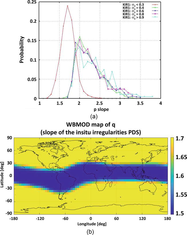
Figure 2.

(a) Measured PDF of the phase spectra slope (p) measured at KIR1 receiver (Kiruna, Sweeden) for different levels of scintillation (σ_ϕ: [0, 0.3], (0.3, 0.5], (0.5, 0.7], (0.7, 0.9], (0.9, ∞), legend indicates central value of the interval). (b) Map of q from WBMOD (p ≈ q + 1). In GISM p = 3.

Its main limitations lie in the fact that the scintillation intensity directly depends on the variance of the electron density at any point and any time in space, which is defined by a constant ratio with respect to the ionosphere electron density mean value provided by NeQuick 2, and that only a mean scintillation level is estimated, without statistical variability. GISM is 2D model, and it does not take into account anisotropies. It is a reliable model for equatorial regions, but it is not usable at high latitudes, as the sensitivity to the magnetic activity (e.g., the geomagnetic K_p index²) is not accounted for (only in the TEC values from NeQuick), and its forecasting performances are limited as it is driven only by the solar flux number F10.7, which is a daily parameter.

• STIPEE [31] proposes a 2D or 3D formulation of the propagation modeling, based on the parabolic wave equation associated with multiple phase screen model (PWE-MPS) or on the Rytov approximation. The medium is described by the Shkarofsky spectrum [32], then anisotropy and medium drift velocity are taken into account. It is reliable for polar and equatorial regions, and it is valid from weak up to strong scintillation if PWE-MPS resolution is used. STIPEE can be used in conjunction with WBMOD (providing C_kL, drift velocity, slope, and anisotropy) to produce time series, or input parameters can be given by the user (electron density variance and ionospheric spectrum parameters, such as drift velocity, slope and anisotropy). At present, a new prediction model has been derived called HAPEE (high latitude scintillation positioning error estimator) and validated [33]. A merger of STIPEE and HAPEE is under construction within a CNES project.

• SCIONAV [34] is a generic model to evaluate the impact of ionospheric disturbances at low and high latitudes, based on physically-based models for low- and high-frequency fluctuations. SCIONAV uses the total electron content (TEC) parametric model from IRI 2016 [35] or NeQuick [23] as a climatologic background, plus a stochastic variability term computed as a mean value plus a uniform random variable computed from LUTs (Look Up Tables) as a function of the year, month, local time, and latitude. These LUTs have been derived by the UPC/gAGE research group [36] after a comprehensive analysis of the VTEC Global Ionospheric Maps (“Final Products”), published by the International GNSS Service (IGS), from 2001 to 2015 (both included) over a 20° × 20° grid. On top of the background and stochastic TEC, based on the statistics of the equatorial plasma bubbles or EPBs observed during the years 2002–2014, an analytical model developed by the Observatori de l’Ebre [37] accounts for the slowly moving ionospheric depletions and bubbles (EPBs) in equatorial regions (low-frequency TEC fluctuations).

The high-frequency fluctuations are modeled at high latitudes (σ_ϕ ≠ 0, S₄ ≈ 0) using a model developed by the UPC/gAGE research group in which the phase scintillation is proportional to the ROTI (Rate Of TEC Index) parameter computed using 1 Hz data [38, 39], and the mapping function (M):

$${\mathrm{\sigma }}_{\mathrm{\varphi }}=\mathrm{\alpha }·M·\mathit{\text{ROTI}}.$$E4

The proportionality constant is α = 0.0555 rad, and the ROTI is sum of three terms:

$$\mathit{\text{ROTI}}={\mathit{\text{ROTI}}}_0+\mathrm{\Delta }\mathit{\text{ROTI}}+{\mathit{\text{ROTI}}}_{\mathrm{off}}$$E5

where ROTI₀ is proportional to the AATR (Along Arc TEC Rate) [40], ΔROTI is a uniform random variable, and ROTI_off ≈ 0.4 TECUs/min, is an offset term.

At equatorial regions, GISM is used to obtain S₄ and σ_ϕ, and the scintillation enhancement due the presence of EPBs is modeled as an increase of the effective S₄ parameter by a factor 1 + C·|ΔSTEC_EPBs(t)|), where ΔSTEC_EPBs is the change in the Slant TEC due to the EPB. Finally, the Cornell Model [41] is used to generate the time series associated to the fast diffractive scintillation.

To summarize, on one side, WBMOD and GISM are both theoretical models calibrated with data on the global morphology of scintillation activity derived from combining measurement data from the VHF and L-band links, but not GNSS data. STIPEE and SCIONAV, being based on WBMOD and GISM inherit the same intrinsic limitations. On the other side, the S₄ model derived from the GNSS radio occultation data from the FormoSat-3/COSMIC mission [14, 15] is a promising empirical model because it includes homogeneous data obtained at global scale, but—to the authors’ knowledge—it still needs to be validated and calibrated using ground-based GPS S₄.

In this study, the goodness of these models is assessed by comparing their outputs to the scintillation parameters measured from a network of GNSS monitoring ground stations. Additionally, these measurements have been used to fine-tune the FormoSat-3/COSMIC S₄ empirical model (or simply COSMIC model in what follows), which can then be used to improve other models in which intensity scintillation is not properly modeled.

2. Methodology and data sets

Performing a validation/verification in the sense of matching model results with experimental data is a necessary proof that the models are correctly developed and implemented, although it might still not be a sufficient proof because experimental data may not be fully representative or suffer from systematic or random errors that would make the model not according to reality, but only according to the reference empirical data set used for model validation. In order to avoid this problem, several steps will be followed, from the simplest case and easier-to-test conditions to increasingly challenging iterations.

Data sets are selected to be as representative as possible according to the following procedure. First, the data will be gathered into four representative regions: Polar caps or PLC (magnetic latitudes greater than 80°), high latitudes or HLT (magnetic latitudes between 70° and 80°), Europe or EUR (excluding the high-latitude regions), and Low/equatorial latitudes or LEQ (±30° around magnetic equator). Second, for each region the data are further divided into severity levels of the observed ionospheric activity: Type 1 corresponding to very high/extreme activity, Type 2 corresponding to moderate to high activity, and Type 3 corresponding to undisturbed ionosphere to low activity. In order to select data for Type 1 scenarios, the events producing the largest AATR values during a full solar cycle period from 2006 to 2016 have been selected. To this end, AATR values were calculated by UPC/gAGE for a network of more than 100 permanent ground stations worldwide distributed. For Type 2 and 3 scenarios, the AATR values were considered for time periods around maximum and minimum solar activity within the interval 2006–2016. In particular, for maximum solar activity, we have focused on the months with average solar flux index F10.7 greater than nearly 150 sfu (solar flux units), which correspond to the periods from November 2013 to April 2014 and from September to December 2014. For minimum solar activity, we have focused on the months with average solar flux index F10.7 smaller than 80 sfu, which are found from February 2007 to December 2009.

Data are provided by different types of ground receivers belonging to two different networks: IGS high-rate geodetic receivers operating at 1-Hz sampling frequency (measurements at intervals of 1 second) and ionospheric scintillation monitor receivers (ISMR) from ESA-MONITOR network [42] providing measurements at 50-Hz sampling frequency (intervals of 0.02 seconds). Part of the data collected from ISMR has been used to verify the reliability of data from 1-Hz geodetic receivers, and another part has been used for model validation, particularly for p-slope (slope of the phase scintillation spectrum) and for S₄ in the equatorial region in South America. Details of which type of data is provided by receivers from the different networks can be found in [38, 39]. Finally, the list of proposed scenarios for model validation based on GNSS data is presented in Table 1.

ID label of; the scenario	Time period				Scenario description
	Year	Day of the Year	LT (h) interval	UT (h); interval	Solar activity	Comments
Type 1 Scenarios
Polar Cap and High-Latitude Regions
GNSS-Typ1-HLT-1	2015	76	—	[15, 19]	High	St. Patrick’s storm
GNSS- Typ1-HLT-2	2014	58	—	[19, 24]	High near maximum	Minor storm but frequent high AATR
GNSS-Typ1-HLT-3	2015	250	—	[15, 24]	High	G2 geomag. Storm
GNSS-Typ1-HLT-4	2015	252	—	[02, 08] & [13, 16]	High	G2 geomag. Storm
Europe Region
GNSS- Typ1-EUR-1	2015	76	—	[15, 19]	High	St. Patrick’s storm
GNSS- Typ1-EUR-2	2014	58	—	[12, 17]	High near maximum	Minor storm but frequent high AATR
Low-Equatorial Regions
GNSS- Typ1-LEQ-1	2014	351	[19, 23]	—	High	Highest AATR in current solar cycle
GNSS- Typ1-LEQ-2	2014	314	[19, 24]	—	High	Activity most equatorial stations
GNSS-Typ1-LEQ-3	2015	298–299	[19, 24]	—	High	Highest activity in days of Set 2
Type 2 Scenarios
Polar Cap and High-Latitude Regions
GNSS- Typ2-HLT-1	2015	291	—	[06, 19]	High	Minor storm. High activity most stations
GNSS- Typ2-HLT-2	2014	62	—	[04, 13]	Near Maximum	High Ionospheric activity
GNSS- Typ2-HLT-3	2007	91	—	[02, 09]	Low near Minimum	Minor storm.
Europe Region
GNSS- Typ2-EUR-1	2014	87	—	[12, 17]	Near Maximum	High Ionospheric activity
GNSS- Typ2-EUR-2	2007	155	[16, 20]	—	Low near Minimum	Moderate Ionospheric activity
GNSS-Typ2-EUR-3	2015	116	[09, 20]	—	High	Highest activity in the region for days of Set 2
GNSS-Typ2-EUR-4	2015	291	[09, 16]	—	High	Minor storm effects in the region
Low-Equatorial Regions
GNSS- Typ2-LEQ-1	2014	87	[19, 24]	—	Near Maximum	High Ionospheric activity
GNSS- Typ2-LEQ-2	2007	80	[19, 24]	—	Low near Minimum	High Ionospheric activity
GNSS-Typ2-LEQ-3	2015	291	[19, 24]	—	High	Only stations in South America & Canary Island
GNSS-Typ2-LEQ-3	2015	115	[19, 24]	—	High	Stations: mal2, dgar, pimo, LOM2, DAK2
Type 3 Scenarios
Polar Cap and High-Latitude Regions
GNSS- Typ3-HLT-1	2014	257	—	[15, 21]	Near Maximum	Low Ionospheric activity
GNSS- Typ3-HLT-2	2007	181	—	[10, 15]	Near Maximum	Low Ionospheric activity
GNSS-Typ3-HLT-3	2015	299	—	[05, 20]	High	Low/Quiet ionospheric activity
Europe Region
GNSS- Typ3-EUR-1	2015	252	[00,09] & [19, 24]	—	High	Quiet Ionosphere nearly all day
GNSS- Typ3-EUR-2	2014	20	[01, 05]	—	Near Maximum	Quiet Ionosphere
GNSS- Typ3-EUR-3	2007	181	—	[10, 15]	Near Maximum	Low Ionospheric activity
Low-Equatorial Regions
GNSS- Typ3-LEQ-1	2015	250–251	[01, 09]	—	High	Quiet Ionosphere, scintillation activity very scarce, the lowest for days in Set 2
GNSS- Typ3-LEQ-2	2014	20	[01, 05]	—	Near Maximum	Quiet Ionosphere
GNSS- Typ3-LEQ-3	2007	181	—	[10, 15]	Near Maximum	Low Ionospheric activity

Table 1.

Consolidated list of GNSS test scenarios.

In the case of the SCIONAV model, a different data set has been used to extract the parameters needed to properly tune the model. Then, these parameters have been organized in different look-up tables (LUTs) by date, latitude, and any other variable that can potentially influence the value of the corresponding parameter (e.g., solar activity). Subsequently, in order to test the model performance, the data set described in Table 1 has been chosen approximately at the same locations and times as the data set used to tune the parameters of the SCIONAV model. Specifically, the GNSS test scenarios in Table 1 are within a range of similar conditions as the data used for model parameter tuning, that is, similar pierce-point locations (elevation angle, magnetic latitude, azimuth direction with regard to solar zenith angle, and magnetic field lines), and similar geomagnetic activity, time-of-day (day/night, close to sunset or not), or conditions depending both of local time and season of the year. In this way, the observed scintillation parameters (S₄, σ_ϕ, ROTI and power spectra slope), and the ionospheric activity index (AATR) can be consistently compared to the scintillation parameters predicted by the original models in similar ionospheric conditions. Note that, the AATR is a widely used indicator of ionospheric activity linked to the local TEC fluctuations observed from GNSS measurements taken by permanent ground receivers. For this reason, it has been used to select the different types of scenarios proposed in the present study according to the level of activity derived by using the AATR thresholds established by [40] for the regions with different ionospheric activity that essentially correspond to the different regions considered in the present work. The AATR has been demonstrated to be correlated with space weather conditions and can be used to monitor planetary storm conditions [43].

Finally, the list of proposed scenarios for model validation based on GNSS data is presented in Table 1.

Note that, for every region, the data are provided by different ground stations at different locations. When the ionospheric activity occurs at a planetary scale, as in the case of some space weather events or geomagnetic storms, the universal time is used to define the data set of the given scenario. Instead, when the ionospheric activity is linked to local times, as in the case of low-latitude scintillation, the scenario is better defined using the local time range, which is relevant at all low-latitude locations.

3. Results

In the next set of plots, the general behavior of the models is compared against the data. Although the plots are divided into geographical regions, they are not subdivided into scintillation categories. Large differences between different low-latitude regions (e.g., between America and Asia/Africa) were not observed in the reference data sets used for model testing, nor in the corresponding model predictions. Therefore, all data from low-latitude regions have been joined in a single set to perform the model analysis.

3.1 S₄ results

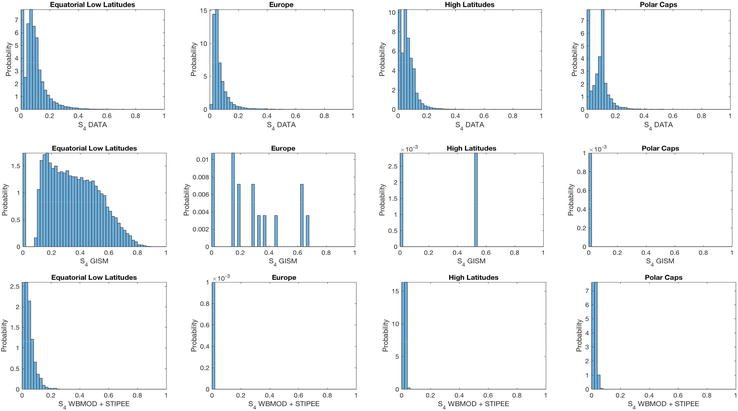
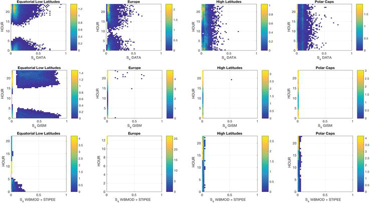
The S₄ model results are only available for GISM and WBMOD, as the SCIONAV model uses the same S₄ as GISM. Results are summarized in Figures 3–5. Figure 3 shows the S₄ PDF in percentage (%) from the ground measurements, from the GISM model, and from the WBMOD + STIPEE model, and per region: equatorial low latitudes, Europe, high latitudes, and polar caps. In the LEQ region, S₄ values have low probability, but they exist, although the scale of the figure does not help to appreciate that. Instead, at PLC and HLT large values of S₄ are not expected since scintillation is mostly refractive and affects the carrier phase but not the signal intensity. Similarly, Figure 4 shows the density plots of S₄ vs. the ROTI, and Figure 5 shows the density plots of S₄ vs. the local time (LT). Note that, in the case of ISMR receivers operating at 50 Hz, the values of σ_ϕ and p are directly outputs of the receivers, while the ROTI is straightforwardly derived from the TEC variations output by the receivers. In the case of geodetic receivers from the IGS network, operating at 1 Hz sampling frequency, the parameters were calculated after processing the carrier phase measurements from the receivers following the Geodetic Detrending methodology as described in Refs. [38, 39].

Figure 3.

PDF [in %] of: (first row) S₄ from the ground measurements (scale normalized to maximum value because of large variations between regions and models), (second row) from the GISM model (SCIONAV has the same output), and (third row) from the WBMOD + STIPEE model, per region.

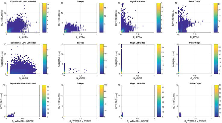
Figure 4.

Density plots of: (first row) S₄ vs. ROTI from the ground measurements, (second row) from the GISM model (SCIONAV has the same output), and (third row) from the WBMOD + STIPEE model, per region. Colorbar indicates percentage.

Figure 5.

Density plots of: (first row) S₄ vs. LT from the ground measurements, (second row) from the GISM model (SCIONAV has the same output), and (third row) from the WBMOD + STIPEE model, per region. Colorbar indicates percentage.

It has been observed in real data that S₄ is correlated with ROTI at low latitudes [44, 45]. However, in Figure 3 model predictions cannot probably reproduce the S₄ data with sufficient accuracy, which is probably responsible of the bad results concerning the S₄-ROTI correlation. As it can be seen, S₄ PDFs from WBMOD+STIPEE are clearly better than those from GISM. However, the dependence with respect to ROTI and LT seems to be better captured by GISM, notably at equatorial regions, not so good at mid-latitudes, and —as expected— not at all at polar regions since it is known that GISM is not modeling properly S₄ at high latitudes.

3.2 σ_ϕ results

The σ_ϕ model results are available for all models, as SCIONAV includes a specific model for the phase scintillation [G. Gonzalez-Casado and J.M. Juan-Zornoza, internal communication, 2016].

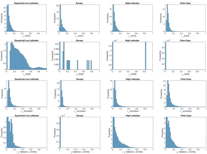
Figure 6 shows the σ_ϕ [in radians] PDF in percentage (%) from the ground measurements, from the GISM model, from the SCIONAV model, and from the WBMOD + STIPEE model, and per region: equatorial low latitudes, Europe, high latitudes, and polar caps. Similarly, Figure 7 shows the density plots of σ_ϕ vs. the ROTI, and Figure 8 shows the density plots of σ_ϕ vs. the local time (LT).

Figure 6.

PDF [in %] of: (first row) σ_ϕ PDF [in %] from the ground measurements (scale normalized to maximum value because of large variations between regions and models), (second row) from the GISM model, (third row) from the SCIONAV model, and (fourth row) from the WBMOD + STIPEE model, per region.

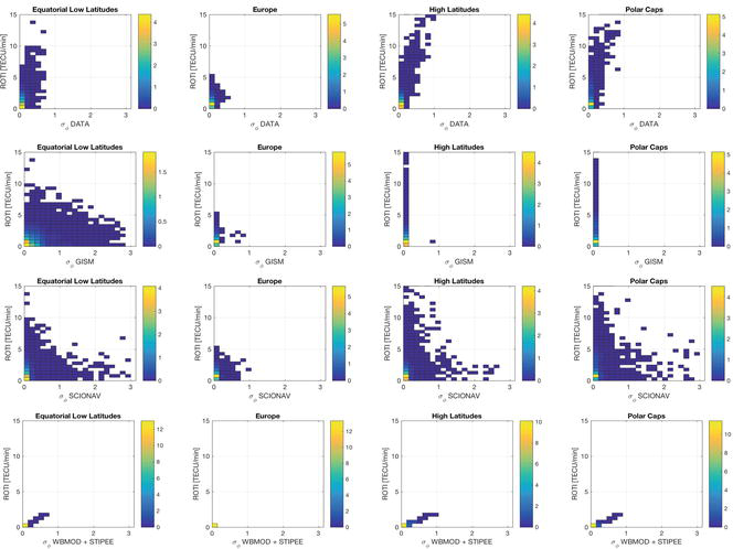
Figure 7.

Density plots of: (first row) σ_ϕ vs. ROTI from the ground measurements, (second row) from the GISM model, (third row) from the SCIONAV model, and (fourth row) from the WBMOD + STIPEE model, per region. Colorbar indicates percentage.

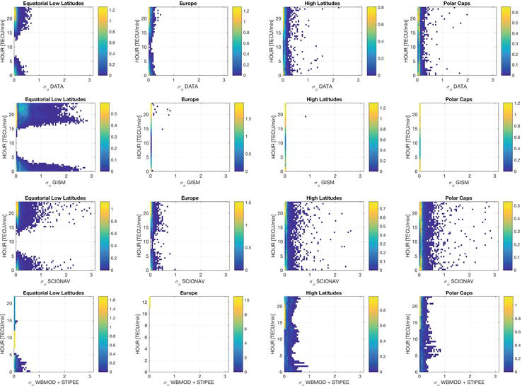
Figure 8.

Density plots of: (first row) σ_ϕ vs. LT from the ground measurements, (second row) from the GISM model, (third row) from the SCIONAV model, and (fourth row) from the WBMOD + STIPEE model, per region. Colorbar indicates percentage.

As it can be seen, σ_ϕ PDFs from SCIONAV are qualitatively better than the other models, WBMOD+STIPEE model being slightly worse than SCIONAV model, as it is a bit wider (i.e., predicts slightly larger σ_ϕ values), and GISM clearly overestimates σ_ϕ, notably at equatorial low latitudes and Europe regions. The dependence with respect to ROTI and LT seems better captured by the SCIONAV model at all latitudes, although some improvements may still be needed at high latitudes to increase the correlation. For WBMOD+STIPEE the correlation is too high, and the dynamic range is too small.

3.3 p-slope results

The p-slope model results are available for SCIONAV and WBMOD+STIPEE models. GISM assumes a constant value of p = 3 [24]. During the analysis of this data, it became apparent that there may be some discrepancies in the definition of the p-slope. On one hand, WBMOD values agree with Beniguel et al. findings [42]. On the other hand, the LUTs used for the p-slope by the SCIONAV model were calculated using values delivered by 50 Hz ISMR from the MONITOR network. In Figure 2a typical p-slope distributions depending on scintillation severity are shown. Figure 2b shows the maps of the q-slope obtained from WBMOD (WBMOD outputs q, being p ∼ q + 1) [22]. As it can be seen, it basically has two values: q = 1.5 at equatorial low-latitude regions and q = 1.7 at mid-to-polar latitudes with a narrow transition zone. Values of p between p = 2.5 and p = 2.7 should then be expected according to WBMOD, but even for high scintillation events, the p-slope values rarely go above 2.5. ISMR observations used to build the distributions shown in Figure 2a show that the probability of p > 2.5 is just around 15–20% for periods of scintillation activity (σ_ϕ > 0.3).

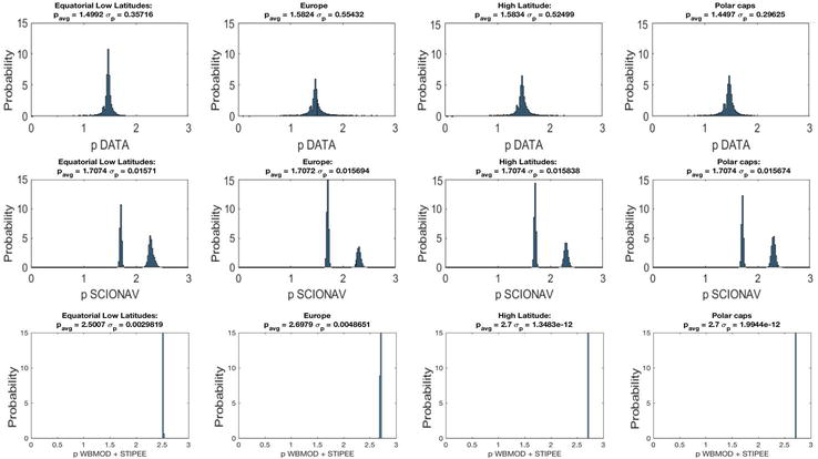
Figure 9 shows the p-slope PDF in percentage from the ground measurements, from the GISM model, from SCIONAV, and from the WBMOD + STIPEE model, and per region: equatorial low latitudes, Europe, high latitudes, and polar caps. Similarly, Figure 10 shows the density plots of p-slope vs. the ROTI, and Figure 11 shows the density plots of p-slope vs. the LT.

Figure 9.

PDF [in %] of: (first row) p-slope PDF from the ground measurements, (second row) from the SCIONAV model, and (third row) from the WBMOD + STIPEE model, per region.

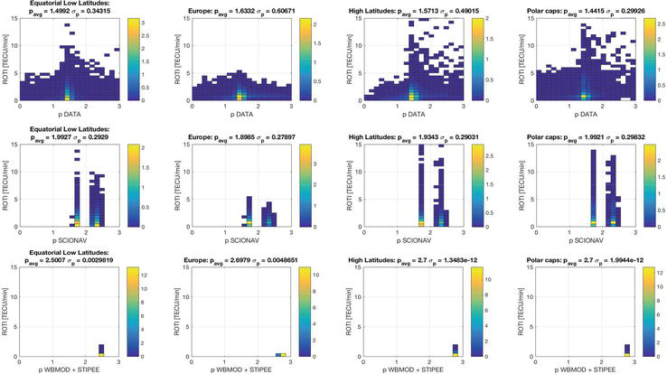
Figure 10.

Density plots of: (first row) p-slope vs. ROTI from the ground measurements, (second row) from the SCIONAV model, and (third row) from the WBMOD + STIPEE model, per region. Colorbar indicates percentage.

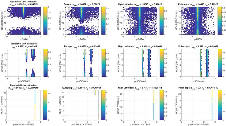
Figure 11.

Density plots of: (first row) p-slope vs. LT from the ground measurements, (second row) from the SCIONAV model, and (third row) from the WBMOD + STIPEE model, per region. Colorbar indicates percentage.

Neither GISM (constant p-value equal to 3, not shown), nor WBMOD (fixed value depending on latitude q ∼ p-1 ∼ 1.5 or 1.7, with narrow transition, Figure 2b), nor SCIONAV exhibit the natural variability, and the variability has to be increased in SCIONAV. When looking at Figures 10 and 11, it can be observed that the p - slope values from SCIONAV exhibit an artificial binomial behavior, which can be attributed to the way the scenarios were selected: groups of low-phase scintillation p ∼ 1.7, and others of high phase scintillation p ∼ 2.3 (see Figure 2a). Apart from that, the SCIONAV model exhibits the correct dependence with ROTI, including the dynamic range and so with LT, which does not seem to be the case of WBMOD+STIPEE.

3.4 Model performance summary

Quantitative results of the previous sections are summarized in Tables 2–4 in terms of the mean and unbiased root mean squared error (uRMSE). A word of caution is given to Table 4 because of the difference in one unit in the definition of the slope (p in all models, and q in WBMOD).

		SCIONAV		GISM		WBMOD + STIPEE
		Mean	uRMS	Mean	uRMS	Mean	uRMS
Low/equatorial; latitudes; (LEQ)	All types	0.1744	0.2166	0.1744	0.2166	−0.0922	0.0783
	Type 1	0.1510	0.2023	0.1510	0.2023	−0.0691	0.0983
	Type 2	0.1957	0.2380	0.1957	0.2380	−0.1771	0.1079
	Type 3	0.2333	0.2237	0.2333	0.2237	−0.0209	0.0230
Europe; (EUR)	All types	−0.0679	0.0553	−0.0679	0.0553	−0.0385	0.0136
	Type 1	—	—	—	—	—	—
	Type 2	−0.0681	0.0557	−0.0681	0.0557	−0.0385	0.0136
	Type 3	—	—	—	—	—	—
High latitudes (HLT)	All types	−0.0575	0.0516	−0.0575	0.0516	−0.0210	0.0263
	Type 1	−0.0585	0.0531	−0.0585	0.0531	−0.0193	0.0269
	Type 2	—	—	—	—	—	—
	Type 3	−0.0557	0.0507	−0.0557	0.0507	−0.0234	0.0251
Polar caps (PLC)	All types	−0.0502	0.0634	−0.0502	0.0634	−0.0922	0.0412
	Type 1	−0.0659	0.0637	−0.0659	0.0637	−0.0246	0.0446
	Type 2	—	—	—	—	—	—
	Type 3	−0.0726	0.0732	−0.0726	0.0732	−0.0283	0.0402

Table 2.

Mean (left) and uRMSE (right) error for S₄. Note: GISM results at high latitudes and polar caps are not meaningful.

Bold type: All types of scenarios; green color: Best results, purple color: Model not applicable

		SCIONAV		GISM		WBMOD + STIPEE
		Mean	uRMS	Mean	uRMS	Mean	uRMS
Low/equatorial latitudes (LEQ)	All types	0.0182	0.1356	0.2133	0.3410	−0.0724	0.0653
	Type 1	0.0484	0.2190	0.1623	0.2437	−0.0434	0.0862
	Type 2	0.0133	0.1085	0.4540	0.5875	−0.1345	0.1051
	Type 3	0.0076	0.0808	0.2907	0.4184	−0.0333	0.0198
Europe (EUR)	All types	−0.0055	0.0629	−0.0541	0.0394	−0.0479	0.0280
	Type 1	—	—	—	—	—	—
	Type 2	−0.0033	0.0610	−0.0522	0.0375	−0.0479	0.0280
	Type 3	—	—	—	—	—	—
High latitudes (HLT)	All types	0.0206	0.1392	−0.0625	0.0643	0.0378	0.1196
	Type 1	0.0563	0.2857	−0.0937	0.1164	0.0730	0.1418
	Type 2	—	—	—	—	—	—
	Type 3	0.0082	0.0663	−0.0502	0.0316	−0.0145	0.0330
Polar caps (PLC)	All types	0.0402	0.1798	−0.0686	0.0542	0.0107	0.0876
	Type 1	0.0599	0.2274	−0.0791	0.0742	0.0458	0.1024
	Type 2	—	—	—	—	—	—
	Type 3	0.0284	0.1151	−0.0650	0.0287	−0.0244	0.0201

Table 3.

Mean (left) and uRMSE (right) error for σ_ϕ.

Bold type: All types of scenarios; green color: Best results, purple color: Model not applicable.

		SCIONAV		WBMOD + STIPEE
		Mean	uRMS	Mean	uRMS
Low/equatorial latitudes (LEQ)	All types	0.4936	0.4538	0.9817	0.3364
	Type 1	0.5188	0.3690	0.9776	0.2787
	Type 2	0.4907	0.3922	0.9620	0.2778
	Type 3	0.4394	0.5271	0.9912	0.386
Europe (EUR)	All types	0.2662	0.6361	1.1162	0.4270
	Type 1	—	—	—	—
	Type 2	0.2904	0.5937	1.1162	0.4270
	Type 3	—	—	—	—
High latitudes (HLT)	All types	0.3639	0.5773	1.0521	0.4992
	Type 1	0.2482	0.5685	0.9713	0.5386
	Type 2	—	—	—	—
	Type 3	0.4257	0.4494	1.1721	0.4054
Polar caps (PLC)	All types	0.5507	0.4285	1.239	0.2985
	Type 1	0.6402	0.4071	1.202	0.3432
	Type 2	—	—	—	—
	Type 3	0.6884	0.3245	1.315	0.2517

Table 4.

Mean (left) and uRMSE (right) error for p-slope.

Bold type: all types of scenarios; green color: best results.

The following conclusions on the models were drawn:

• S₄ modeling analysis:

  • GISM does not seem to have a good S₄ model when compared against the data or against WBMOD. It provides artificially high values of S_4, and it is also known to lack a proper model at high latitudes (results in purple in Table 2). It is the same for SCIONAV, which is based on GISM.

  • WBMOD+STIPEE has a more realistic distribution, even if it produces values slightly lower than reality.

  • While it has been observed in real data that S₄ is correlated with ROTI at low latitudes [40, 42], this correlation is not captured by any model. This is a motivation to investigate the performance of the COSMIC model in order to improve the S₄ modeling.

  • GISM and WBMOD models account properly for the dependence with LT.

  • In this study, SCIONAV model has the bubbles and depletions code deactivated, so the estimated S₄ values would be slightly higher.

• σ_ϕ modeling analysis:

  • GISM models artificially high values of σ_ϕ.

  • SCIONAV model exhibits a very good agreement with data in terms of mean and standard deviation, for all regions, types of events, and LT.

  • WBMOD model is very good, but in some cases, it does not reproduce so well the dispersion with LT, and it has lower error dispersion across regions.

• p-slope modeling analysis:

  • GISM uses a default value of p = 3.

  • WBMOD uses a fixed value depending on latitude (q = 1.5 at equatorial low latitudes, or q = 1.7 at mid-to-polar latitudes; so p ∼ q + 1 = 2.5–2.7).

  • SCIONAV modeled p-slope PDF depends on σ_ϕ (Figure 2a)_. The bimodality presented could be caused by the simplicity of the modeling based on the PDFs presented in Figure 2a, and/or by the selection of the data in extreme cases.

  • Additionally, estimated values of p from real data are biased towards lower values because of the limitations of the IGS 1 Hz data, which does not sample the full spectra of phase fluctuations.

  • The p-slope is not the best-suited parameter to assess the performance analysis of the models considered in the present study.

4. Discussion and way forward

4.1 Summary of the experimental results

So far, the assessment of model performance was done using GNSS data (i.e., L-band). A fundamental point to keep in mind is the difference modeling philosophy in the four models.

Whereas GISM and SCIONAV are providing a mean level of scintillation along each link, WBMOD and STIPEE are considering the statistics of occurrence of an event, or a scintillation index value for a given percentile. In order to compare the different models, WBMOD/STIPEE results have been estimated at a percentile 50.

One additional important point is that the models’ inputs are different. Along Arc TEC Rate (AATR) scintillation index is used as input for SCIONAV to characterize the phase scintillation, whereas WBMOD is using the Kp index, which is not a scintillation index, it is a geomagnetic index derived from the standardized K-index of 13 magnetic observatories, and it is designed to measure the solar particle radiation by its magnetic effects. In this way the approaches of the models are different, WBMOD being a blind model considering ionosphere scintillation input but considering magnetic conditions instead.

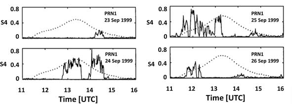
GISM results have been assumed as a mean level of scintillation. This assumption has been taken to compare the model with measurements, but it can be discussed. The problem remains in the definition, and in the derivation of the climatologic part of the models that have not been well described by the models. WBMOD is based on a statistical approach, considering that for a given ionospheric conditions (date, local time, solar exposure, latitude, and magnetic conditions) the scintillation intensity may change with time. An illustration is displayed in Figure 12, representing ISMR S₄ data measured in Parepare, Indonesia, and the corresponding WBMOD prediction at the ninetieth percentile. Four consecutive days have been chosen in September 1999. These plots demonstrate the “patchy” nature of scintillation in contrast to WBMOD, which produces smooth predictions of scintillation for a given percentile. WBMOD, such as all other models proposed in this study, is not able to reproduce the night-to-night variability of scintillation activity. This variable behavior of the measurements indicates that a statistical approach seems to be required to model scintillation.

Figure 12.

Comparison between ISMR S₄ (solid line) data and WBMOD predictions at 90 percentile (dotted line) on five separate days in September 1999 for GPS satellite Pseudo-Random code Number (PRN) 1 observed at Parepare, Indonesia (adapted from [19]).

Medium anisotropy influence is of high importance for SAR modeling, and it has also an impact on GNSS links. WBMOD is proposing a parametrization of anisotropy in terms of the along-field: (a) across field and (b) axial ratios, with values from ∼10–50 and ∼ 1–4, respectively. These variables exhibit a smooth evolution with the local solar time (LST) and K_p, but no dependence with the Day of the Year (DoY), the twelve-month smoothed relative sunspot number (R12), or the percentile. However, this remains hard to validate.

In a conclusion, as it has been shown, while the phase scintillations are reasonably well characterized by both SCIONAV and WBMOD+STIPEE models (see Table 3), large errors occur in S₄ in GISM and SCIONAV, which is based on GISM for S₄ (see Table 2). Hence, any potential model improvement in S₄ predictions should be very relevant and will help to improve the overall accuracy.

4.2 S₄ model improvement

In the following paragraphs, an attempt to improve the S₄ modeling is described using the semiempirical model developed in [14, 15] to convert the 3D FORMOSAT-3/COSMIC or F3/C S_{4, max} (maximum value on each profile) into a 2D latitude and longitude S₄-index map on the ground has been used (hereafter called S₄-index).

The scintillation model can be subdivided into low-latitude and high-latitude parts, which are connected/overlapped between ±45° and ± 65° dip. The model combines a constant low-latitude weight, between −45° and 45° dip latitudes, and a constant high- latitude weight, below −65° and above 65° dip latitude, with linear transitions between those two regions in the middle latitudes in both hemispheres. For each region, the model is composed of the product of four terms [15], the Diurnal one, $S_{\mathit{\text{Diur}}}$, the annual one, $S_{\mathit{\text{An}}}$, the one that models the latitudinal (dip) variations, $S_{\mathit{Dip}}$, and the one that depends on the solar flux, $S_{\mathit{PF}10.7}$, as shown below:

$$S_4=S_{\mathit{\text{Diur}}}\left(\mathit{LT}\right)·S_{\mathit{\text{An}}}\left(\mathit{DoY},\mathit{lon}\right)·S_{\mathit{Dip}}\left(\mathit{Dip}\right)·S_{\mathit{PF}10.7}\left(\mathit{YY},\mathit{DoY},\mathit{PF}10.7\right)·k+S_{4,\mathit{\text{bias}}}.$$E6

In (Eq. (6)) the term YY, DoY, and LT are the Year, Day of the Year and local time, is the PF107 = (F10.7+ F10.7A)/2, being F10.7 the solar flux daily value, and F10.7A the 81-day running mean value of the solar radio flux at 10.7 cm wavelength, respectively.

Originally, the model used k = 0.78125 and S_4,bias = 0.07. However, to achieve consistency with the ground GNSS data set used for model testing (Table 1); in the present study, two of the parameters of the model, the calibration constant k and the bias term S_4,bias have been adjusted to minimize the rms error to the values shown in Table 5. The remaining parameters and functionalities introduced in [15] have not been modified. Note that biases are negligible, but values of k are much larger than in [15].

	LEQ	EUR	HLT	PLC
K	7.9902	25.6787	8.9855	9.5047
S4,bias	−0.0058	−0.0000	−0.0000	−0.0000

Table 5.

Optimum values of k and S_4,bias for each region: equatorial and low latitudes (LEQ), Europe (EUR), high latitudes (HLT), and polar caps (PLC).

Values obtained by minimized rms error between experimental data (Table 1) and COSMIC model.

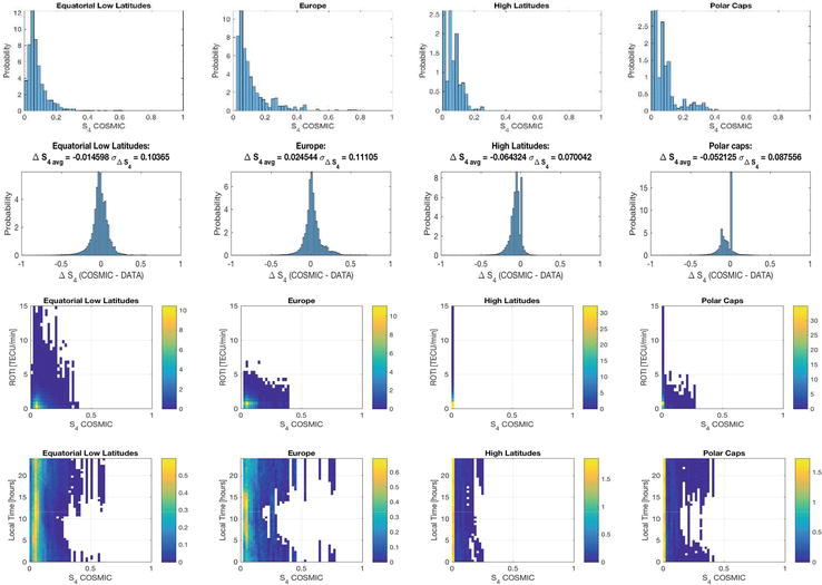
Figure 13 shows the performance of the COSMIC model in terms of the S₄ PDF, S₄ error PDF, the density plots of S₄ vs. ROTI, and the density plots of S₄ vs. LT, per region. Clearly, COSMIC S₄ PDFs seem better than from GISM/SCIONAV, with a noticeable improvement at equatorial regions. ROTI dependence seems also better behaved with COSMIC S₄, except at high latitudes. Finally, LT dependence seems also better behaved with COSMIC, at all latitudes. Additionally, the error histograms (second row) are more symmetric and Gaussian-like than for other models (not shown), despite the rms is slightly larger —except in LEQ region—, which is an indication that the model is properly modeling the nature of the statistics of the ionospheric intensity scintillations.

Figure 13.

Performance of COSMIC model: (first row) S₄ PDF, (second row) S₄ error PDF, (third row) S₄ vs. ROTI, and (fourth row) S₄ vs. LT, per region. Colorbar indicates percentage.

5. Conclusions

This chapter has summarized the outcomes of an ESA study to analyze the performance of several ionospheric scintillation models and to provide recommendations for future improvements. The models analyzed are GISM, SCIONAV, WBMOD, STIPEE, and COSMIC. The analysis has been performed using S₄, σ_ϕ, and p for the first four and, only S₄ for COSMIC, derived from GNSS data from ground stations. Data have been binned by regions: equatorial and low latitudes, Europe and mid-latitudes, high latitudes, and polar caps.

Table 6 summarizes the main parameters of S₄ for all regions, types of scintillation, and models. The GISM model (and SCIONAV, as it uses GISM inside to compute S₄) is not appropriate for high latitudes and polar regions, in terms of S₄. The best results are obtained with a tuned COSMIC model (bias and gain factor) for all regions, except for high latitudes where the WBMOD+STIPEE model outperforms. This is possibly due to the lower data sampling used to derive the COSMIC model.

S4	SCIONAV/GISM		WBMOD + STIPEE		COSMIC
	Mean	RMS	Mean	RMS	Mean	RMS
Low/equatorial latitudes (LEQ)	0.1744	0.2166	−0.0922	0.0783	−0.0146	0.1037
Europe (EUR)	−0.0679	0.0553	−0.0385	0.0136	0.0245	0.1110
High Latitudes (HLT)	−0.0575	0.0516	−0.0210	0.0263	-0.0643	0.0700
Polar Caps (PLC)	−0.0502	0.0634	−0.0922	0.0412	−0.0521	0.0876

Table 6.

Summary of mean and uRMS error for S₄ for all types, regions, and models.

Bold type: all types of scenarios; green color: best results, red color: worst results, purple color: model not applicable. Recall that SCIONAV uses GISM S₄ as an input.

In terms of σ_ϕ, the best results are obtained by SCIONAV’s phase scintillation model, except for polar caps, where WBMOD slightly outperforms. WBMOD outperforms always in terms of the uRMSE.

Finally, in terms of p, SCIONAV model outperforms in terms of the average error, but WBMOD+STIPEE in terms of the uRMSE. Improved modeling of p is still required.

Tuning of the COSMIC S₄ empirical model to the data collected (Table 1) has led to the lowest average errors (except for WBMOD at high latitudes). It could be used in conjunction with the SCIONAV σ_ϕ model to better model the ionospheric scintillation behavior.

Future work must be conducted to improve/update the characterization of the patchy behavior of the ionosphere, assess the validity of some approximations of the models, such as the constant slope and the anisotropy… and implement a 4D (3D + time) simulator of the ionospheric scintillation, including ionospheric drifts.

Acknowledgments

This research was funded by the project “Radio Climatology Models of the Ionosphere: Status and Way Forward,” ESA/ESTEC, grant number 4000120868/17/NL/AF [https://nebula.esa.int/content/radio-climatology-models-ionosphere-status-and-way-forward]. Article processing charges were funded by the project “GENESIS: GNSS Environmental and Societal Missions – Subproject UPC,” AEI Grant PID2021-126436OB-C21.

IGS data were available from: https://cddis.nasa.gov/archive/gnss/data/highrate/. MONITOR data were provided by ESA. WBMOD simulations were performed by ONERA; GNSS ground stations data processing was performed by UPC/gAGE, and GISM and SCIONAV simulations were performed by UPC/CommSensLab-IEEC.

Conflict of interest

The authors declare no conflict of interest.