The Application of Markov and Semi-Markov Models in Transportation Infrastructure Management

Abstract

This chapter outlines how Markov and semi-Markov models can be used in Transportation Infrastructure Management Systems, in particular Pavement and Bridge Management Systems. The use of Markov models have been used in both Pavement and Bridge Management Systems for years. In more recent times the use of semi-Markov models have been introduced in Bridge Management Systems. Research has shown that if there is enough data available to develop semi-Markov models for transportation infrastructure, then this stochastic technique can be used to predict the future network level conditions and can be used in the development of preservation models for transportation infrastructure. The application of these techniques are not only limited to transportation infrastructure, but can also be applied in other areas.

1. Introduction

This chapter demonstrates how Markov and semi-Markov models are used in Transportation Infrastructure Management. Transportation agencies are interested in being able to model the deterioration of their infrastructure when no action is taken to neither maintain, repair nor rehabilitate that infrastructure. The Transportation agencies also want to know how to best estimate the extension in the service life of an infrastructure when improvement actions (maintenance, repair or rehabilitation) are done. The chapter uses examples containing real life data to demonstrate models for the following actions: deterioration or ‘do-nothing’ actions, improvement action and rehabilitation.

Markov chain has been used to model the performance of pavements in Pavement Management Systems (PMSs), such as The Arizona Department of Transportation (ADOT) Network Optimization System (NOS) [1, 2]. Wang et al. [2] outlined an approach to compute the transition probabilities of a Markov chain model using pavement performance data. Nasseri et al. [3] used Markov chain applications to investigate the crack histories of flexible pavements and to deduce the cause of rapid deterioration of surface cracks. Markov chain can also be used to model the deterioration of other infrastructures, including bridge elements, storm water pipes and wastewater pipes [4, 5, 6]. Yang et al. [7, 8] mentioned the use of semi-Markov processes for modeling the crack performance of flexible pavements, as a precursor to outlining how recurrent Markov chains can be used to model crack performance of flexible pavements. Semi-Markov processes are used in the deterioration models for other assets such as bridge elements and transformers [9, 10, 11, 12]. Although sections 2 and 3 in this chapter uses pavement condition data to describe the application of stochastic processes for ‘do-nothing’ actions, the techniques can be applied to other transportation infrastructure, such as bridge elements [13].

2. Markov chain model

This section demonstrates a Markov chain model for flexible (asphalt) road pavement. The stochastic process, known as the Markov chain [14], can be described as follows: If $X_n=i$ describes a process such that the process is in state i at time n, and the process in state i has a fixed probability $P_{i,j}$ of being in state j, after a transition, then

$$P\left\{X_{n+1}=j|X_n=i,X_{n-1}=i_{n-1},\dots ,X_0=i_0\right\}=P_{i,j}$$E1

for all states $i_0,i_1,\stackrel{⌣}{U}{i}_{n-1},i,j$ and all $n\ge 0$.

Consider the range of crack indices associated with flexible (asphalt) road pavement that have been assigned the respective condition states in the Table 1. The following equation, used by Wang et al. [2], can be used to generate transition probabilities for a Markov chain model:

Crack Index (CRK) range	Condition state
$9.5\le \mathit{CRK}\le 10$	10
$8.5\le \mathit{CRK}<9.5$	9
$7.5\le \mathit{CRK}<8.5$	8
$6.5\le \mathit{CRK}<7.5$	7
$5.5\le \mathit{CRK}<6.5$	6
$4.5\le \mathit{CRK}<5.5$	5
$\mathit{CRK}<4.5$	4

Table 1.

The range of crack indices and corresponding condition states.

$$p_{i,j}\left(a_k\right)=\frac{m_{i,j\left(a_k\right)}}{m_i\left(a_k\right)}$$E2

for $i,j=\mathrm{10,9,8,7,6,5}\&4$ where,

• k = k^th rehabilitation action, in this case, the ‘do-nothing’ action, i.e. k = 1.

• $p_{i,j}\left(a_k\right)$ = transition probability from state i to j after action k is taken.

• $m_{i,j}\left(a_k\right)$ = total number of miles of pavement for which the state prior to action k was i and the state after the action k was j.

• $m_i\left(a_k\right)$ = total number of miles of pavement for which the state prior to action k was i.

3. Semi-Markov model

This section demonstrates a Semi-Markov model for flexible (asphalt) road pavement. Consider a stochastic process having states $\mathrm{0,1,2},\dots ,$ which is such that whenever it enters state $i,i\ge 0$, then: (1) it will enter the next state j with probability $P_{\mathit{ij}},i,j,\ge 0$, and (2) given that the next state is j the sojourn time from i to j has distribution $F_{\mathit{ij}}$. For a semi-Markov process, the sojourn times may follow a specific distribution and the method of Maximum Likelihood Estimation (MLE) can be used to estimate the parameters of that distribution, such as that of a Weibull Distribution [13]. Before discussing how the semi-Markov process can be applied to model deterioration, it is beneficial to define the basic concepts of the MLE method. The Maximum Likelihood is a well-known technique in statistics used for deriving estimators [15].

3.1 Maximum likelihood estimation

If there is an identical and independently distributed (iid) sample, $X_1,\dots ,X_n$ from a population with probability density function (pdf) or probability mass function (pmf) $f\left(x|{\theta }_1,\stackrel{⌣}{U}{\theta }_k\right)$, then the likelihood function is defined by

$$L\left(\theta |X\right)=L\left({\theta }_1,\dots ,{\theta }_k|x_1,\dots ,x_n\right)={\mathrm{\Pi }}_{i=1}^{n}f\left(x_i|{\theta }_1,\dots ,{\theta }_k\right)$$E3

Let us assume that the sojourn time follows a Weibull Distribution. The pdf of the Weibull distribution according to Billington and Allan [16], Tobias and Trindade [17] is defined by:

$$f\left(t\right)=\frac{\beta }{\alpha }{\left(\frac{t}{\alpha }\right)}^{\beta -1}{e}^{-{\left(\frac{t}{\alpha }\right)}^{\beta }}$$E4

where $\alpha$ and $\beta$ are the respective scale and shape parameters, and t represents the number of years that each unit of a mile of pavement segment takes to sojourn in one condition state before transitioning to another state. If $\eta =1/\alpha$, then

$$f\left(t\right)=\mathit{\beta \eta }{\left(\mathit{\eta t}\right)}^{\beta -1}{e}^{-{\left(\mathit{\eta t}\right)}^{\beta }}$$E5

Using Eq. 3 [18] it follows that the likelihood is:

$$L\left(t_1,\dots ,t_n,\eta ,\beta \right)={\left({\mathit{\beta \eta }}^{\beta }\right)}^n{e}^{-{\eta }^{\beta }}\left(t_1^{\beta }+\dots +t_n^{\beta }\right){\mathrm{\Pi }}_{i=1}^n{t}_i^{\beta -1}$$E6

After differentiating the log likelihood and equating it to zero, the MLE of the parameters $\widehat{\beta }$ and $\widehat{\eta }$ are:

$$\widehat{\beta }={\left[\frac{{\sum }_{i=1}^n{t}_i^{\widehat{\beta }}\mathit{ln}\left(t_i\right)}{{\sum }_{i=1}^n{t}_i^{\widehat{\beta }}}-\frac{1}{n}\sum _{i=1}^n\mathit{ln}\left(t_i\right)\right]}^{-1}$$E7

and

$$\widehat{\eta }={\left[\frac{n}{{\sum }_{i=1}^n{t}_i^{\widehat{\beta }}}\right]}^{1/\widehat{\beta }}$$E8

respectively.

If there are n units of pavement in a particular condition state and k units have transitioned to a lower condition state (with complete individual sojourn times $t_1<t_2<\dots <t_k$) and the sojourn time for $n-k$ units of pavement are not known, then the sojourn times $T_1,\dots ,T_n-k$ for the $n-k$ units of pavement should also be accounted for in the evaluation [13]. For the Weibull distribution, if it is assumed that the incomplete sojourn times of $T_1,\dots ,T_{n-k}$ have been observed in addition to the complete sojourn times $t_1,\dots ,t_k$, then the likelihood function can be expressed as:

$$L=\underset{i=1}{\overset{k}{\mathrm{\Pi }}}f\left(t_i|\theta \right)\cdot {\mathrm{\Pi }}_{j=1}^{n-k}f\left(1-F\left(T_j,|\theta \right)\right)$$E9

where i sums over all completed sojourn times, j sums over all incomplete sojourn times, and $\theta$ can be a vector [13].

$$L\left(t_1,\dots ,t_n,\eta ,\beta \right)={\left({\mathit{\beta \eta }}^{\beta }\right)}^k{e}^{-{\eta }^{\beta }}\left(t_1^{\beta }+\dots +t_k^{\beta }\right){\mathrm{\Pi }}_{i=1}^k{t}_i^{\beta -1}{\mathrm{\Pi }}_{j=1}^{n-k}{e}^{-{\left(\eta T_j\right)}^{\beta }}$$E10

producing the MLE of the parameters $\widehat{\beta }$ and $\widehat{\eta }$:

$$\widehat{\beta }={\left[\frac{{\sum }_{i=1}^k{t}_i^{\widehat{\beta }}\mathit{ln}\left(t_i\right)+{\sum }_{j=1}^{n-k}{T}_j^{\widehat{\beta }}\mathit{ln}\left(T_j\right)}{{\sum }_{i=1}^k{t}_i^{\widehat{\beta }}+{\sum }_{j=1}^{n-k}{T}_j^{\widehat{\beta }}}-\frac{1}{k}\sum _{i=1}^k\mathit{ln}\left(t_i\right)\right]}^{-1}$$E11

and

$$\widehat{\eta }={\left[\frac{k}{{\sum }_{i=1}^k{t}_i^{\widehat{\beta }}+{\sum }^{n-k}{k}_{i=1}{T}_j^{\widehat{\beta }}}\right]}^{1/\widehat{\beta }}$$E12

3.2 Semi-Markov Kernel

To demonstrate how the semi-Markov can be developed by knowing the sojourn times in a particular condition state before transitioning, one may consider the semi-Markov kernel in the form shown in Eq. 13. Ibe [19] defines the one-step transition probability $Q_{i,j}\left(t\right)$ of the semi-Markov process as:

$$Q_{i,j}\left(t\right)=P\left[X_{n+1}=j,G_n\le t|X_n=i\right]t\ge 0$$E13

where $Q_{i,j}\left(t\right)$ is the conditional probability that the process will be in state j next, given that it is in state i currently and that the waiting time in the current state i is no more than t. $G_n$ is the time the process spends in i before transitioning to j. It also follows that:

$$Q_{i,j}\left(t\right)=p_{i,j}{H}_{i,j}\left(t\right)$$E14

where $p_{i,j}$ is defined as the transition probability of the embedded Markov chain, and

$$H_{i,j}\left(t\right)=P\left[G_n\le t|X_n=i,X_{n+1}=j\right]$$E15

3.2.1 Semi-Markov process

Howard [20] provided the following formulation to determine the probability that a continuous-time semi-Markov process will be in state j at time n given that it entered state i at time zero.

$$\begin{array}{l}{\varphi }_{\mathit{ij}}\left(n\right)={{\delta }_{\mathit{ij}}}^{>}{w}_i\left(n\right)+\sum _{k=1}^N{p}_{\mathit{ik}}{\int }_0^n{h}_{\mathit{ik}}\left(m\right){\varphi }_{\mathit{kj}}\left(n-m\right)i=1,2,\dots ,N;j=1,2,\dots ,N;\\ n=\mathrm{0,1,2},\\ \dots \end{array}$$E16

$${\delta }_{\mathit{ij}}=\left\{\begin{array}{ll}1& i=j;\\ 0& i\ne j.\end{array}\right.$$E17

where ${\varphi }_{\mathit{ij}}\left(n\right)$ is the probability that a continuous-time semi-Markov process will be in state j at time n given that it entered state i at time $n=0$ and is referred to as the interval transition probability from state i to state j in the interval $\left(0,n\right)$. ${}^{>}{w}_i\left(n\right)$ is the probability that the process will exit its starting state i at a time greater than n.

The second term in 3.2.1 describes the probability of the sequence of events, such that the process makes an initial transition from state i to some state k at some time m and thereafter proceeds from state k to state j in the remaining time n–m. To account for all possible scenarios, the probability is summed over all states k to which the first transition could have been made and over all times of the initial transition, m, between l and n. $p_{\mathit{ik}}$ is the probability of transitioning from i to k, and $h_{\mathit{ik}}\left(m\right)$ represents the probability distribution of the sojourn time from i to k at time m. The matrix formulation of 3.2.1 can be expressed as:

$$\mathrm{\Phi }\left(n\right){=}^{>}W\left(n\right)+{\int }_0^n\left[P\square H\left(m\right)\right]\mathrm{\Phi }\left(n-m\right)n=\mathrm{0,1,2},\dots$$E18

In addition, let

$$C\left(m\right)=\left[P\square H\left(m\right)\right]$$E19

where C(m) is defined as the core matrix [20]. The elements of $C\left(m\right)$ are $c_{\mathit{ij}}\left(m\right)=p_{\mathit{ij}}{h}_{\mathit{ij}}\left(m\right)$, where $p_{\mathit{ij}}$ represents the transition probability of the embedded Markov chain and $h_{\mathit{ij}}\left(m\right)$ represents the probability distribution of the sojourn time in state i, before transitioning to j at time m.

As a result, the interval transition matrix representing a single transition at time m, ${\mathrm{\Phi }}^{0,m}\left(m\right)$, for ‘do-nothing’ actions can be expressed as:

$${\mathrm{\Phi }}^{0,m}\left(m\right)=\left(\begin{array}{ccccccc}1-{\sum }_{j=4}^9{p}_{10,j}{H}_{10,j}\left(m\right)& \dots & \dots & \dots & \dots & p_{10,5}{H}_{10,5}\left(m\right)& p_{10,4}{H}_{10,4}\left(m\right)\\ 0& \ddots & \dots & \dots & \dots & p_{9,5}{H}_{9,5}\left(m\right)& p_{9,4}{H}_{9,4}\left(m\right)\\ 0& 0& \ddots & \dots & \dots & p_{8,5}{H}_{8,5}\left(m\right)& p_{8,4}{H}_{8,4}\left(m\right)\\ 0& 0& 0& \ddots & \dots & p_{7,5}{H}_{7,5}\left(m\right)& p_{7,4}{H}_{7,4}\left(m\right)\\ 0& 0& 0& 0& \ddots & p_{6,5}{H}_{6,5}\left(m\right)& p_{6,4}{H}_{6,4}\left(m\right)\\ 0& 0& 0& 0& 0& 1-p_{5,4}{H}_{5,4}\left(m\right)& p_{5,4}{H}_{5,4}\left(m\right)\\ 0& 0& 0& 0& 0& 0& 1\end{array}\right)$$E20

where $p_{\mathit{ij}}$ represents the probability for the embedded Markov chain of the semi-Markov process, and $H_{\mathit{ij}}$ represents the cumulative distribution of the sojourn time between condition state i and condition state j at time m.

It can be seen by 3.2.1 that as the number of years, m, increases, a number of permutations must be considered when computing the overall transition probabilities for an interval $\left(0,n\right)$, and so another approach is suggested to model the overall transition over time. In the context of modeling asset deterioration, the focus is on ‘do-nothing’ scenarios, where there is no action taken on the infrastructure. It therefore can be assumed that once the infrastructure exits a condition state, that condition state is not visited again, and the semi-Markov process occurs in one direction only. There is also the probability of the condition of some infrastructure, in this case the pavement segments, ‘skipping’ condition states in a single transition, however the probability of ‘skipping’ two (2) or more condition states is extremely small and therefore may not have to be considered. If it is assumed that only one condition state may be ‘skipped’ in a single transition, then the transition probability (for the embedded Markov chain), $p_{\mathit{ij}}$, of ‘skipping’ a condition state, k, is one minus the transition probability (for the embedded Markov chain) of transitioning to the next state, $p_{\mathit{ik}}$. Therefore,

$$p_{\mathit{ij}}=1-p_{\mathit{ik}}i=\mathrm{10,9,8,7,6,5};j=i-2,k=i-1,\mathit{min}\left(j,k\right)=4$$E21

This is because the total probability of eventually leaving a particular condition state (which is not a terminal state), to a lower condition state is 1, since deterioration is being considered.

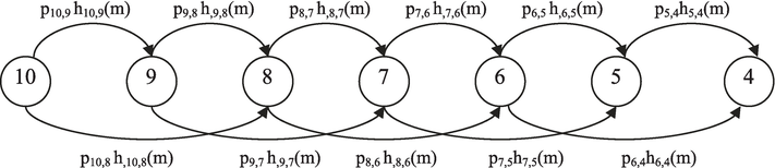
Another assumption is that the sojourn time in condition state i before transitioning to j is the time from the pavement segment first entered condition state i to the time the pavement segment first entered condition state j. The transition diagram shown in Figure 1 shows the possible ‘single step’ transitions in developing the semi-Markov model, where $p_{\mathit{ij}}$ is the probability for the embedded Markov chain from condition state i to condition state j, and $h_{\mathit{ij}}\left(m\right)$ is the probability density function of the sojourn time between condition state i and condition state j at time m. The term ‘single step’ transition is based on the assumption that only a single transition can take place in a year. For the transition labeled $p_{10,9}{h}_{10,9}\left(m\right)$ the pavement segment spends some time in condition state 10 before transitioning to condition state 9, and for the transition labeled $p_{10,8}{h}_{10,8}\left(m\right)$ the pavement segment spends some time in condition state 10 before transitioning to condition state 8 without going to 9 [13].

Figure 1.

Transition diagram that represents the possible ‘single step’ transitions between condition states.

Other than determining the interval transition probabilities for the interval $\left(0,n\right)$, the conditional transition probabilities for each yearly interval for $m=1,2,\dots ,n$ is determined, which is multiplied by each other to estimate the transition probabilities for the interval $\left(0,n\right)$. It is also assumed that only a single transition takes place in a year. In other words, let

$${\mathrm{\Phi }}^{0,n}\left(n\right)={\mathrm{\Phi }}^{0,1}\cdot {\mathrm{\Phi }}^{1,2}\cdot \dots {\mathrm{\Phi }}^{n-1,n}$$E22

where ${\mathrm{\Phi }}^{m-1,m}$ is a 1 year ‘single’ transition probability matrix for the time $m-1$ to m (i.e. $m^{\mathit{th}}$ interval), $m=1,2,\dots ,n$. Based on Eq. (20), if the condition states can drop by either one (1) or two (2) states, then the interval transition probability for the first year results to:

$${\mathrm{\Phi }}^{0,m}\left(m\right)=\left(\begin{array}{ccccccc}1-{\sum }_{j=8}^9{p}_{10,j}{H}_{10,j}\left(m\right)& p_{10,9}{H}_{10,9}\left(m\right)& p_{10,8}{H}_{10,8}\left(m\right)& 0& 0& 0& 0\\ 0& \ddots & \dots & \dots & 0& 0& 0\\ 0& 0& \ddots & \dots & \dots & 0& 0\\ 0& 0& 0& \ddots & \dots & \dots & 0\\ 0& 0& 0& 0& \ddots & \dots & \dots \\ 0& 0& 0& 0& 0& \ddots & \dots \\ 0& 0& 0& 0& 0& 0& 1\end{array}\right)$$E23

where $m=1$. On the other hand, to determine the respective transition probability matrices for the subsequent intervals, a different formulation is used, in which it is assumed that the sojourn time is left truncated at the start of each interval.

3.2.2 Service life analysis and left truncation

Statistical analyses of the service lives of transportation infrastructures can be done using Reliability Theory otherwise called Survival Analysis. In Survival Analysis, sometimes subjects are selected and followed prospectively until the event or censoring occurs, but sometimes the start time at the point of selection is not $t=0$ (i.e. not at birth), but at a value $t=t_0>0$. It therefore means that the life or censoring time of the subjects, $T_i$, is greater than $t_0$ [21, 22], and the life $T_i$ is considered to be left truncated at $t_0$. Applying the same principle to the service life of a transportation infrastructure then,

$$F_{T\mid T>t_0}\left(t\right)=\left\{\begin{array}{ll}0& \mathit{\text{if}}{t}_0\ge t;\\ \frac{F_T\left(t\right)-F_T\left(t_0\right)}{1-F_T\left(t_0\right)}& \mathit{\text{if}}{t}_0<t.\end{array}\right.$$E24

To determine the probabilities that are associated with the sojourn time for interval $\left(1,2\right]$, we assume that from Eq. (24) $t_0=1$ and $1<t\le 2$. It therefore means that at this point only sojourn times greater than $t=1$ are being considered and the cumulative distribution of the sojourn time in the interval can be considered truncated [22]. It is therefore can be described as:

$$H_{i,j_{T\mid T>1}}\left(t\right)=\frac{H_{i,j_T}\left(t\right)-H_{i,j_T}\left(1\right)}{1-H_{i,j_T}\left(1\right)},1<t\le 2$$E25

It follows that for interval $\left(m-1,m\right]$ the cumulative distribution of the sojourn time in the interval can be described as:

$$H_{i,j_{T\mid T>m-1}}\left(t\right)=\frac{H_{i,j_T}\left(t\right)-H_{i,j_T}\left(m-1\right)}{1-H_{i,j_T}\left(m-1\right)},m-1<t\le m$$E26

At $t=m$ the cumulative distribution of the sojourn time then becomes

$$H_{i,j_{T\mid T>m-1}}\left(m\right)=\frac{H_{i,j_T}\left(m\right)-H_{i,j_T}\left(m-1\right)}{1-H_{i,j_T}\left(m-1\right)},m-1<t\le m$$E27

Therefore, the transition probability for interval $\left(m-1,m\right]$ is:

$${\mathrm{\Phi }}^{m-1,m}\left(m\right)=\left(\begin{array}{ccccccc}1-{\sum }_{j=8}^9{p}_{10,j}{H}_{10,j_{T|T>m-1}}\left(m\right)& p_{10,9}{H}_{10,9_{T|T>m-1}}\left(m\right)& \dots & 0& 0& 0& 0\\ 0& \ddots & \dots & \dots & 0& 0& 0\\ 0& 0& \ddots & \dots & \dots & 0& 0\\ 0& 0& 0& \ddots & \dots & \dots & 0\\ 0& 0& 0& 0& \ddots & \dots & \dots \\ 0& 0& 0& 0& 0& \ddots & \dots \\ 0& 0& 0& 0& 0& 0& 1\end{array}\right)$$E28

Eq. (27) have been used to determine the transition probabilities for one-step state-based yearly transitions in deterioration models by Black et al. [11, 12], for which the transition probability of the embedded Markov chain was assumed to be 1. It therefore means that the probability obtained using Eq. (27) can be used to describe the probability associated with the sojourn time to the end of the period, given that it had ‘survived’ up to the start of the period.

3.2.3 Sojourn times of flexible pavement condition states

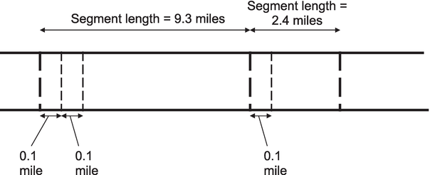
For developing the semi-Markov model, the number of miles for a particular segment can be rounded to the nearest one-tenth of a mile and the sojourn time distribution for each one-tenth unit of a mile of pavement segment is then analyzed. Figure 2 gives a schematic of how the pavement segment can be divided into one-tenth of a mile sub-sections. An algorithm can be created and used to help organize and analyze the data on the infrastructure to estimate the parameters of the sojourn time distributions in each condition state. The following outlines the steps:

1. The length of each segment to the nearest one-tenth of a mile is determined.

2. The yearly decreases in CRKs for each segment subsequent to the year being newly constructed or overlaid is extracted, such that a series of decreasing CRKs for each segment can be used to model ‘do-nothing’ actions on the pavement segments over time.

3. The pavement segments are assigned to condition states over time, in accordance with Table 1, as outlined earlier.

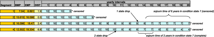
4. At some point in time, all the pavement segments tracked, are either just becoming ‘new’ or entered the current condition state from a higher or equal condition state. If a unit of pavement segment exits a particular condition state to a lower condition state at a known time, then the sojourn time of that unit of pavement segment in the current condition state is essentially known. However, if a unit of pavement segment is in a particular condition state and the tracking of the pavement ended because the condition state either increased or the because the ‘study’ was terminated, then the sojourn time of that unit of pavement segment is not precisely known and is considered right-censored [23]. Figure 3 gives a representation of the change in the condition states of pavement segments over time, outlining examples of complete and censored times spent in particular condition states.

5. Based on the complete and censored durations obtained from the data, the distribution of the sojourn time in condition state i before transitioning to condition state j ($H_{i,j}\left(t\right)$) can be determined, where j is either $i-1$ or $i-2$, $i=\mathrm{10,9,8,7,6,5}\mathit{min}\left(j\right)=4$. The proportion of the number of units of the infrastructure that left condition state i and transitioned to condition state j, to the total number of units of assets that left condition state i and transitioned to all condition states other than itself ($p_{i,j}$) can be determined, for each condition state i. From Figure 3, one can see that segment 3 spends 6 years in condition state 10, has a one state drop and then spends 7 years in condition state 9, and then has another one state drop to condition state 8. It shows that segment 3 then spends 1 year in condition state 8, before transitioning to condition state 7, where the pavement segment spent at least 6 years in condition state 7. In Figure 3, for segment 4, it is seen that the segment spends 10 years in condition state 10 before having a two-state drop to condition state 8, followed by a series of one state drops for which the respective sojourn times can also be inferred.

Figure 2.

Schematic of pavement segment divisions into equal units of one-tenth of a mile.

Figure 3.

An example of the change in the condition states of pavement segments over time.

The maximum likelihood estimate of the scale ($\alpha$) and shape ($\beta$) parameters of the Weibull distribution, used to describe the sojourn time distributions, can be computed. An algorithm can be written to determine the series of transition probability matrices, based on the Weibull parameters ($\alpha$ and $\beta$ values) obtained for the sojourn times between condition states. The MLE of the $\alpha$ and $\beta$ values serves as inputs for this algorithm. The transition probabilities according to Eqs. (23) and (28) can then be determined and used to simulate the survival curves and the expected deterioration over time.

4. Examples of transition probabilities associated with the Markov chain and semi-Markov models

4.1 Transition probabilities in a Markov chain model

An example of a set of transition probabilities for a Markov chain model are represented as a transition probability matrix, as shown below in Eq. (29). At the left and top of the transition probability matrix in Eq. (29) are the condition states i and j respectively, where ${\mathrm{\Pi }}_{\mathit{ij}}$ is transition probability matrix used for a Markov chain model.

$$\begin{array}{l}10987654\\ {\mathrm{\Pi }}_{\mathit{ij}}=\begin{array}{c}10\\ 9\\ 8\\ 7\\ 6\\ 5\\ 4\end{array}\left(\begin{array}{ccccccc}0.905& 0.072& 0.017& 0.006& 0& 0& 0\\ 0& 0.737& 0.157& 0.090& 0.016& 0& 0\\ 0& 0& 0.660& 0.274& 0.042& 0.014& 0.010\\ 0& 0& 0& 0.707& 0.188& 0.086& 0.019\\ 0& 0& 0& 0& 0.724& 0.112& 0.164\\ 0& 0& 0& 0& 0& 0.582& 0.418\\ 0& 0& 0& 0& 0& 0& 1\end{array}\right).\end{array}$$E29

4.2 Transition probabilities in a semi-Markov model

An example of the transition probability of the embedded Markov chain of a semi-Markov process are shown for each transition in Table 2.

Transitions i to j	Transition probability
10 to 9	0.707
9 to 8	0.752
8 to 7	0.645
7 to 6	0.468
6 to 5	0.214
5 to 4	1.000
10 to 8	0.293
9 to 7	0.248
8 to 6	0.355
7 to 5	0.532
6 to 4	0.786

Table 2.

Transition probabilities of the embedded Markov chain of the semi-Markov process.

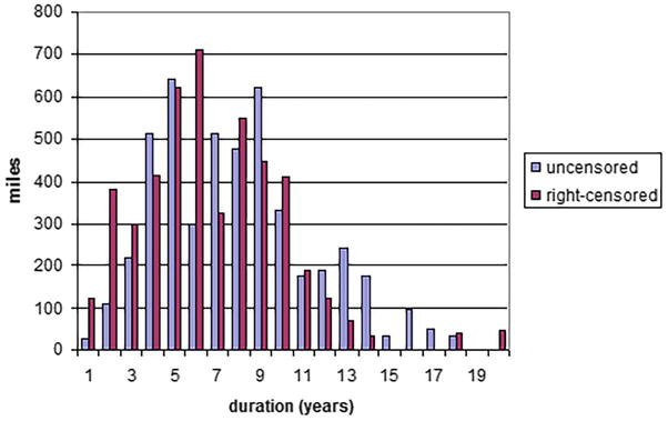
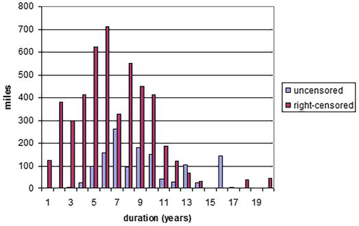
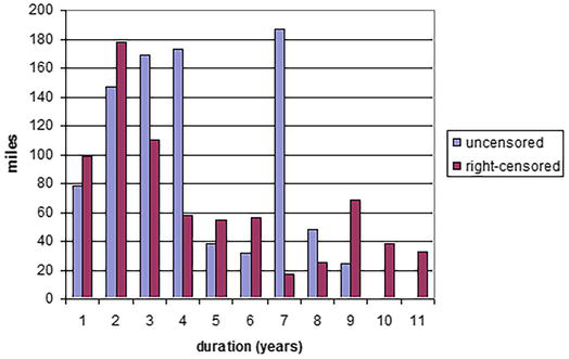
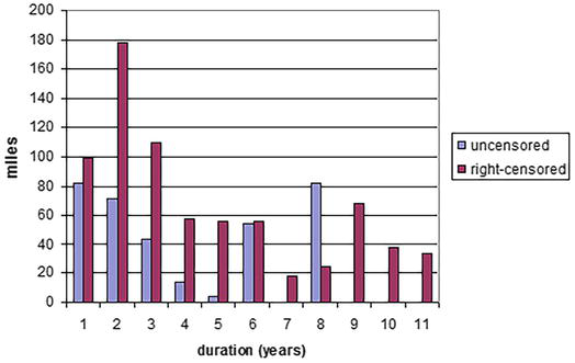
Figures 4–7 show examples of the frequency distributions of the observed sojourn time for each unit mile before transition, including both the uncensored and right-censored sojourn times.

Figure 4.

Frequency of sojourn times in condition state 10 before transitioning to 9.

Figure 5.

Frequency of sojourn times in condition state 10 before transitioning to 8.

Figure 6.

Frequency of sojourn times in condition state 9 before transitioning to 8.

Figure 7.

Frequency of sojourn times in condition state 9 before transitioning to 7.

From Figures 4 and 5 it can be seen that there are more units of pavement that transitioned completely from condition state 10 to 9, than from 10 to 8, which is expected. The total pavement length that are right-censored in Figures 4 and 5 are the same. This is because it is not known whether each unit of pavement would have transitioned from condition state 10 to 9 or from 10 to 8.

Based on the Maximum Likelihood Estimation (MLE), examples of the Weibull distribution parameters are shown in Table 3, while the associated uncertainties are illustrated in Table 4. The 95% C.I. limits of the scale and shape parameters are shown in Table 3. Table 4 provides the means and standard deviations for each sojourn time (Weibull) distribution. The standard deviations for the sojourn time in condition state 8 before transitioning to 6, and that of condition state 7 before transitioning to 5 seems relatively high in comparison to the others, which is a function of the quantity of data representing each transition. As more data for each transition becomes available, then the standard deviations associated with the particular transition is expected to be less. A Goodness-of-fit test can also be done on the distribution of the complete sojourn times.

Transition $i$ to $j$	$\widehat{\alpha }$	95% C.I. limits for $\widehat{\alpha }$		$\widehat{\beta }$	95% C.I. limits for $\widehat{\beta }$
		Lower	Upper		Lower	Upper
10 to 9	9.432	9.332	9.533	2.128	2.094	2.163
9 to 8	4.887	4.777	4.999	1.579	1.539	1.62
8 to 7	3.496	3.394	3.602	1.345	1.304	1.387
7 to 6	5.039	4.811	5.278	1.257	1.208	1.308
6 to 5	6.304	5.754	6.906	1.523	1.412	1.641
5 to 4	3.164	3.03	3.304	2.062	1.94	2.193
10 to 8	13.126	12.904	13.351	3.182	3.088	3.278
9 to 7	6.103	5.845	6.372	1.249	1.204	1.295
8 to 6	9.672	8.744	10.697	1.465	1.35	1.591
7 to 5	9.103	8.355	9.918	1.236	1.165	1.312
6 to 4	5.417	5.092	5.763	1.693	1.591	1.802

Table 3.

Example of the maximum likelihood estimation of the scale ($\alpha$) and shape ($\beta$) parameters for the holding time (Weibull) distributions in condition state i.

Transitions $i$ to $j$	Mean (years)	Standard deviation
10 to 9	8.35	4.13
9 to 8	4.39	2.84
8 to 7	3.21	2.41
7 to 6	4.69	3.75
6 to 5	5.68	3.80
5 to 4	2.80	1.43
10 to 8	11.75	4.05
9 to 7	5.69	4.58
8 to 6	8.76	6.08
7 to 5	8.50	6.91
6 to 4	4.84	2.94

Table 4.

Means and standard deviations of sojourn times (Weibull).

As an example, the transition probability matrices of the first 5 years for the semi-Markov model are shown in Eqs. (30)–(34). In Eq. (30), ${\varphi }_{10,10}=0.991$ means that there is a 0.991 probability that the pavement segment remains in condition state 10. The other ${\varphi }_{i,j}$ terms represent the probability of transition from $i$ to $j$ in a given year.

Year 1

$$\begin{array}{l}10987654\\ {\mathrm{\Phi }}_{\mathit{ij}}\left(1\right)=\begin{array}{c}10\\ 9\\ 8\\ 7\\ 6\\ 5\\ 4\end{array}\left(\begin{array}{ccccccc}0.991& 0.008& 0.001& 0& 0& 0& 0\\ 0& 0.822& 0.078& 0.100& 0& 0& 0\\ 0& 0& 0.795& 0.170& 0.035& 0& 0\\ 0& 0& 0& 0.814& 0.123& 0.063& 0\\ 0& 0& 0& 0& 0.886& 0.059& 0.056\\ 0& 0& 0& 0& 0& 0.911& 0.089\\ 0& 0& 0& 0& 0& 0& 1\end{array}\right).\end{array}$$E30

Year 2

$$\begin{array}{l}10987654\\ {\mathrm{\Phi }}_{\mathit{ij}}\left(2\right)=\begin{array}{c}10\\ 9\\ 8\\ 7\\ 6\\ 5\\ 4\end{array}\left(\begin{array}{ccccccc}0.970& 0.028& 0.002& 0& 0& 0& 0\\ 0& 0.716& 0.150& 0.134& 0& 0& 0\\ 0& 0& 0.690& 0.249& 0.061& 0& 0\\ 0& 0& 0& 0.749& 0.166& 0.085& 0\\ 0& 0& 0& 0& 0.773& 0.107& 0.120\\ 0& 0& 0& 0& 0& 0.744& 0.256\\ 0& 0& 0& 0& 0& 0& 1\end{array}\right).\end{array}$$E31

Year 3

$$\begin{array}{l}10987654\\ {\mathrm{\Phi }}_{\mathit{ij}}\left(3\right)=\begin{array}{c}10\\ 9\\ 8\\ 7\\ 6\\ 5\\ 4\end{array}\left(\begin{array}{ccccccc}0.944& 0.049& 0.007& 0& 0& 0& 0\\ 0& 0.652& 0.197& 0.151& 0& 0& 0\\ 0& 0& 0.633& 0.290& 0.077& 0& 0\\ 0& 0& 0& 0.717& 0.188& 0.095& 0\\ 0& 0& 0& 0& 0.695& 0.138& 0.167\\ 0& 0& 0& 0& 0& 0.602& 0.398\\ 0& 0& 0& 0& 0& 0& 1\end{array}\right).\end{array}$$E32

Year 4

$$\begin{array}{l}10987654\\ {\mathrm{\Phi }}_{\mathit{ij}}\left(4\right)=\begin{array}{c}10\\ 9\\ 8\\ 7\\ 6\\ 5\\ 4\end{array}\left(\begin{array}{ccccccc}0.915& 0.071& 0.014& 0& 0& 0& 0\\ 0& 0.603& 0.234& 0.163& 0& 0& 0\\ 0& 0& 0.591& 0.319& 0.090& 0& 0\\ 0& 0& 0& 0.694& 0.203& 0.103& 0\\ 0& 0& 0& 0& 0.631& 0.163& 0.206\\ 0& 0& 0& 0& 0& 0.484& 0.516\\ 0& 0& 0& 0& 0& 0& 1\end{array}\right).\end{array}$$E33

Year 5

$$\begin{array}{l}10987654\\ {\mathrm{\Phi }}_{\mathit{ij}}\left(5\right)=\begin{array}{c}10\\ 9\\ 8\\ 7\\ 6\\ 5\\ 4\end{array}\left(\begin{array}{ccccccc}0.883& 0.093& 0.024& 0& 0& 0& 0\\ 0& 0.562& 0.265& 0.173& 0& 0& 0\\ 0& 0& 0.557& 0.343& 0.100& 0& 0\\ 0& 0& 0& 0.676& 0.215& 0.109& 0\\ 0& 0& 0& 0& 0.577& 0.183& 0.240\\ 0& 0& 0& 0& 0& 0.388& 0.612\\ 0& 0& 0& 0& 0& 0& 1\end{array}\right).\end{array}$$E34

5. Stochastic preservation model

This section outlines a stochastic preservation model based on bridge elements. The model can be used for transportation infrastructure management, in which the underlining decision model is based on a semi-Markov decision process (SMDP). The “Bare Concrete Deck” is an example of a bridge element that has different condition states to which the preservation model can be applied in a Bridge Management System. The preservation model is adaptive and this concept has been used by researchers in the field of infrastructure management, particularly as it relates to pavement and rail infrastructures [24, 25, 26, 27]. Madanat et al. [27] also describes the methodology used in the Pontis^® Bridge Management System as being adaptive, since transition probabilities are updated over time. The methodology outlined here is based on the application of SMDP.

The maintenance activities on a bridge element can encompass a wide range of types of work having varying durations. Again, the Weibull distribution can be assumed to estimate the sojourn time, which in this case, is the time it takes for maintenance actions to be completed. Unlike the ‘do-nothing’ action, it is assumed that the sojourn times for maintenance activities are irrespective of the current and subsequent condition states of the bridge element. It can also be assumed that rehabilitation works predominantly encompass the replacement of the respective bridge element, which has a more predictable duration time than that of maintenance works. The time taken for improvement (maintenance and rehabilitation) works to be completed, can be interpreted to start from the point at which the problem to the bridge element was first identified, including the time for the required works to be sent out for bid if necessary, followed by the time taken to undertake the works.

5.1 Network level optimization

One of the main goals of a Bridge Management System (BMS) is to be able to determine the minimum-cost long-term policy for each bridge element [28]. This policy consists of a set of recommended actions that minimizes the long-term Maintenance, Repair and Rehabilitation (MR&R) cost requirements, while keeping the bridge element out of risk of failure. If the minimum-cost long-term policy can be determined, it represents the most cost-efficient set of actions for the bridge element. Therefore, if any of the actions are delayed, it results in more expense in the long-term. Also, if more improvement actions other than what is recommended are done, then it will also result in higher costs in the long-term. This is based on the steady state concept. Bridge elements are expected to remain in service for long periods of time providing transportation connectivity on a continuous basis. Having an optimal policy that is sustainable far into the future is of great importance. In a BMS the following three (3) things typically takes place each year: (1) Bridge elements deteriorate when no improvement actions are done to them, otherwise called ‘do-nothing’ actions; (2) Improvement actions are done to some of the bridge elements, which results in corresponding costs; and (3) The improvement actions cause an overall improvement in network conditions [13].

At the network level, any given condition state will have elements passing in and out of condition states based on the MR&R actions. For steady state to occur across the entire bridge network or across a subset of that network, the total quantity of bridge element entering a particular condition state is equal to the total quantity of that similar bridge element leaving that same condition state. As a result the distribution of a bridge element among its condition state remains constant from year to year within the group, and the policy becomes sustainable over the long-term [28]. The optimal policy is the one policy that satisfies the requirements of a steady state and consequently minimizes annual expenditure of the transportation agency in charge of MR&R works.

The Markov Decision Process MDP have been used in the Pontis Bridge Management System to determine the optimal policy, in which there is a means to update the transition probabilities over time or as needed. This is because a Markov chain model assumes that the sojourn time in one state before transitioning to another follows an exponential distribution for continuous time, thus making it more restrictive than the semi-Markov process in which the sojourn times can be assumed to follow a different distribution, such as the Weibull distribution. The SMDP facilitates the natural updating or changing of the transition probabilities over time. Again, it is assumed that the sojourn time in a particular condition state follows the Weibull distribution, and the deterioration process can be represented as a semi-Markov process. The probability density function (pdf) for the Weibull distribution is [29]:

$$f\left(t\right)=\frac{\beta }{\alpha }{\left(\frac{t}{\alpha }\right)}^{\beta -1}{e}^{-{\left(\frac{t}{\alpha }\right)}^{\beta }}$$E35

where $\alpha$ and are the scale and shape parameters respectively. When the shape parameter equals 1, the resulting distribution becomes exponential, and the rate deterioration is constant. If the shape parameter is greater than 1, it means that the rate of deterioration increases with time, and if the shape parameter is less than 1, the rate of deterioration decreases with time. Typically, the latter is not expected for transportation infrastructure.

One component of the preservation model for bridge elements is the deterioration model similar to that explained above, where the Maximum Likelihood Estimation of the parameters of the Weibull distribution, used to describe the sojourn time in one condition state before transitioning to a lower condition state, is determined. A similar approach can be used to determine the sojourn time distribution for maintenance works.

5.2 Discount coefficient

Let us consider continuous-time discounting at a rate $s>0$, such that the present value of one unit received $t$ times units in the future equals $e^{-\mathit{st}}$. For discounting over 1 year, let $t=1$, therefore, $e^{-s}=d$, where $d$ represents corresponding discrete-time discount rate that would be used in a MDP. So, for example, $d=0.9$ in the MDP corresponds to $s=-\mathit{log}\left(0.9\right)=0.105$ in the SMDP, which is the corresponding discount factor based on continuous-time [30].

5.3 The Laplace transform (s-transform)

When taking into consideration the discounting for continuous-time in the SMDP model, the Laplace transform (s-transform) of the distribution of the sojourn times between states has to be computed [19]. It is therefore prudent to look at Laplace transform. Now, if is the pdf of a continuous random variable $X$ that takes only non-negative values; then $f_X\left(x\right)=0$ for $x<0$. It follows that the Laplace transform of $f_X\left(x\right)$, denoted by $M_x\left(s\right)$ is [19]:

$$M_x\left(s\right)=E\left[e^{-\mathit{sX}}\right]={\int }_0^{\infty }{e}^{-\mathit{sx}}{f}_x\left(x\right)\mathit{dx}$$E36

An essential Laplace transform property is that when it is evaluated at s = 0, its value is equal to 1:

$${\left.M_x\left(s\right)\right|}_{s=0}={\int }_0^{\infty }{f}_x\left(x\right)\mathit{dx}=1$$E37

The Laplace transform of the Weibull distribution can be complex, as shown in Eq. (38) [31].

$$E\left[e^{-\mathit{tX}}\right]=\frac{1}{{\lambda }^k{t}^k}\frac{p^k\sqrt{q/p}}{{\left(\sqrt{2\pi }\right)}^{q+p-2}}{G}_{p,q}^{q,p}\left(\begin{array}{c}\frac{1-k}{p},\frac{2-k}{p},\dots ,\frac{p-k}{p}\\ \frac{0}{q},\frac{1}{q},\dots ,\frac{q-1}{q}\end{array}|\frac{p^p}{{\left(q{\lambda }^k{t}^k\right)}^q}\right)$$E38

where G is known as the Meijer G-function.

As a result, it may have to be solved numerically. The numerical solutions are determined by substituting the scale and shape (Weibull) parameter estimates and the continuous-time discount rate, $s$, into the expression provided in Eq. (39).

$$M_x\left(s\right)=E\left[e^{-\mathit{sX}}\right]={\int }_0^{\infty }{e}^{-\mathit{sx}}\cdot \frac{\beta }{\alpha }{\left(\frac{t}{\alpha }\right)}^{\beta -1}{e}^{-{\left(\frac{t}{\alpha }\right)}^{\beta }}\mathit{dx}$$E39

For the case of when the bridge element condition is in the terminal state, mathematically, it can be assumed that the bridge element spends 1 year in that state before ‘transitioning’ back into the terminal state. When a particular transition takes 1 year every time, then the equivalent to the Laplace transform in this scenario is provided by Eq. (40) [30]:

$$M_x\left(s\right)=E\left[e^{-\mathit{sX}}\right]=e^{-s}$$E40

5.4 Semi-Markov decision process with discounting

The computation of the present values based on the SMDP is provided by the following formulation [19, 20]:

$$v_i\left(a,\lambda \right)=r_i\left(a,\lambda \right)+\sum _{j=1}^N{p}_{\mathit{ij}}\left(a\right){\int }_{\tau =0}^{\infty }{v}_j\left(a,\lambda \right)e^{-\mathit{\lambda \tau }}{f}_{H_{\mathit{ij}}}\left(\tau ,a\right)\mathit{d\tau }i=1,\dots ,N$$E41

where, $v_i\left(a,\lambda \right)$ = total expected long-term discounted cost; $i$ = the condition state of a bridge element; $a$ = set of feasible MR&R actions for condition state $i$; $r_i\left(a,\lambda \right)$ = the expected cost for an MR&R action $a$ in condition state $i$; $\lambda$ = the continuous-time discount factor; $p_{\mathit{ij}}\left(a\right)$ = the transition probability of the embedded Markov chain that the bridge element will transition from condition state $i$ to condition state $j$ after action $a$ is taken; $f_{H_{\mathit{ij}}}$ is the probability density function of the sojourn time, $\tau$, from condition state $i$ to condition state $j$, when action $a$ is taken. Therefore,

$$v_i\left(a,\lambda \right)=r_i\left(a,\lambda \right)+\sum _{j=1}^N{p}_{\mathit{ij}}\left(a\right)M_{\mathit{ij}}^H\left(a,\lambda \right)v_j\left(a,\lambda \right)$$E42

where $M_{\mathit{ij}}^H\left(a,\lambda \right)$ is the Laplace transform (s-transform) of $f_{H_{\mathit{ij}}}\left(\tau ,a\right)$ evaluated at $s=\lambda$, and transition probability matrix, $P_{i,j}$ is given by,

$$P_{i,j}\left(a\right)=\left[\begin{array}{ccccc}{p}_{1,1}\left(a\right)& p_{1,2}\left(a\right)& \dots & \dots & p_{1,N}\left(a\right)\\ p_{2,1}\left(a\right)& p_{2,2}\left(a\right)& \dots & \dots & p_{2,N}\left(a\right)\\ \dots & \dots & \dots & \dots & \dots \\ p_{N-1,1}\left(a\right)& p_{N-1,2}\left(a\right)& \dots & \dots & p_{N-1,N}\left(a\right)\\ p_{N,1}\left(a\right)& p_{N,2}\left(a\right)& \dots & \dots & p_{N,N}\left(a\right)\end{array}\right]$$E43

If we let

$$q_{\mathit{ij}}\left(a,\lambda \right)=p_{\mathit{ij}}\left(a\right)M_{\mathit{ij}}^H\left(a,\lambda \right)$$E44

we obtain

$$v_i\left(a,\lambda \right)=r_i\left(a,\lambda \right)+\sum _{j=1}^N{q}_i\left(a,\lambda \right)v_j\left(a,\lambda \right)i=1,\dots ,N.$$E45

According to [19], the long-term value for $r_i\left(a,\lambda \right)$ is given by

$$=B_i\left(a\right)+\sum _{j=1}^N{p}_{\mathit{ij}}{\int }_{\tau =0}^{\infty }{\int }_{x=0}^t{e}^{-\mathit{\lambda x}}{b}_{\mathit{ij}}\left(x,a\right)f_{H_{\mathit{ij}}}\left(\tau ,a\right)\mathit{\text{dxdτ}}$$E46

where $B_i\left(a\right)$ is the immediate cost and is determined by

$$B_i\left(a\right)=\sum _{j=1}^N{p}_{\mathit{ij}}\left(a\right)B_{\mathit{ij}}\left(a\right)i=1,\dots ,N{B}_{\mathit{ij}}\left(a\right)<\infty$$E47

Mathematically, the second term in Eq. (46) represents the sum of the costs that accumulates at the rate per unit time until the transition to state $j$ occurs, $b_{\mathit{ij}}\left(x,a\right)<\infty$. For the SMDP model, it is assumed that only ‘immediate’ costs are incurred when there is a transition from one condition state to another. It can therefore be assumed that the second term in Eq. (46) equals zero. Expressing Eq. (45) in a matrix form, we have [19]:

$$V\left(a,\lambda \right)={\left[v_1\left(a,\lambda \right)v(a,\lambda )\dots v(a,\lambda )\right]}^T$$E48

$$R\left(a,\lambda \right)=V\left(a,\lambda \right)={\left[\begin{array}{cccc}{r}_1\left(a,\lambda \right)& r_2\left(a,\lambda \right)& \dots & r_N\left(a,\lambda \right)\end{array}\right]}^T$$E49

$$Q\left(a,\lambda \right)={\left[\begin{array}{cccc}{q}_{1,1}\left(a,\lambda \right)& q_{1,2}\left(a,\lambda \right)& \dots & q_{1,N}\left(a,\lambda \right)\\ q_{2,1}\left(a,\lambda \right)& q_{2,2}\left(a,\lambda \right)& \dots & q_{2,N}\left(a,\lambda \right)\\ \dots & \dots & \dots & \dots \\ q_{N,1}\left(a,\lambda \right)& q_{N,2}\left(a,\lambda \right)& \dots & q_{N,N}\left(a,\lambda \right)\end{array}\right]}^T$$E50

Based on Eq. (45), considering steady state conditions,

$$V\left(a,\lambda \right)=R\left(a,\lambda \right)+Q\left(a,\lambda \right)V\left(a,\lambda \right)$$E51

then,

$$V\left(a,\lambda \right)={\left[I-Q\left(a,\lambda \right)\right]}^{-1}R\left(a,\lambda \right)$$E52

As a result, there is a $Q\left(a,\lambda \right)$ that gives the minimum long-term cost, which is based on an optimum policy. The minimum long-term cost is defined by Ibe [19] as:

$$v_i^{\ast }=\mathit{min}\left\{r_i\left(a,\lambda \right)+\sum _{j=1}^N{q}_{\mathit{ij}}(a,\lambda \left)v_j^{\ast }\right(a,\lambda )\right\}i=1,\dots ,N$$E53

5.5 Do-nothing action (action ‘$d$’)

As mentioned before, for ‘do-nothing’ actions ($a_d$) it can be assumed that the sojourn time in a condition state before transition, follows a Weibull distribution, except when sojourning in the terminal state. Using Eq. (39), the numerical solution for the Laplace of the Weibull distribution for each scenario, except failure, can be determined. Let:

$$M_{\mathit{ij}}^H\left(a_d,\lambda \right)=L\left\{f\left(\infty ,a_d|{\alpha }_{\mathit{ij}},{\beta }_{\mathit{ij}}\right)\right\}i,j=1,\dots ,\mathit{NS}$$E54

where NS represents the number of states, not including the terminal state. The terminal state can be referred to an absorption condition state or the point at which the bridge element has come to the end of its useful life. In other words, when considering the ‘do-nothing’ action on a bridge element, once the condition state enters the terminal state, it will remain in that state unless rehabilitated. It follows that,

$$M_{\mathit{ij}}^H\left(a_d,\lambda \right)=e^{-s}=e^{-\lambda }s=\lambda ;i=j=F$$E55

where $F$ represents the terminal state. From Eqs. (44), (50) and (54),

$$Q\left(a_d,\lambda \right)=\left[\begin{array}{cccc}{p}_{1,1}\cdot L\left\{f\left(\infty ,a_d|{\alpha }_{1,1},{\beta }_{1,1}\right)\right\}& \dots & \dots & p_{1,F}\cdot L\left\{f\left(\infty ,a_d|{\alpha }_{1,F},{\beta }_{1,F}\right)\right\}\\ ⋮& \dots & \dots & ⋮\\ p_{F,1}\cdot L\left\{f\left(\infty ,a_d|{\alpha }_{F,1},{\beta }_{F,1}\right)\right\}& \dots & \dots & p_{F,F}\cdot L\left\{f\left(\infty ,a_d|{\alpha }_{F,F},{\beta }_{F,F}\right)\right\}\\ 0& 0& 0& e^{-\lambda }\end{array}\right]$$E56

where $a_d$ represents ‘do-nothing’ action.

It can be assumed that the deterioration of bridge elements is a one-step process, and the bridge element can only drop by one condition state at a given point in time. In other words, a bridge element in a particular condition state will eventually transition to the next lower condition state when there are no other actions on that element other than ‘do-nothing’ actions. It can also assumed that for ‘do-nothing’ actions, once the condition of the bridge element exits a condition state, that condition state will not be visited again. The transition probability for the embedded Markov chain of the semi-Markov process, $p_{\mathit{ij}}$, for ‘do-nothing’ action is therefore assumed to be 1 between the current and succeeding condition states, and for the terminal state. Therefore, for the bridge element that has five (5) condition states plus the terminal state,

$$P_{i,j}\left(a_d\right)=\left[\begin{array}{cccccc}0& 1& 0& 0& 0& 0\\ 0& 0& 1& 0& 0& 0\\ 0& 0& 0& 1& 0& 0\\ 0& 0& 0& 0& 1& 0\\ 0& 0& 0& 0& 0& 1\\ 0& 0& 0& 0& 0& 1\end{array}\right]$$E57

and so Eq. (56) can be simplified to:

$$Q\left(a_d,\lambda \right)=\left[\begin{array}{cccccc}0& L\left\{f\left(\infty ,a_d|{\alpha }_{1,2},{\beta }_{1,2}\right)\right\}& 0& 0& 0& 0\\ 0& 0& L\left\{f\left(\infty ,a_d|{\alpha }_{2,3},{\beta }_{2,3}\right)\right\}& 0& 0& 0\\ 0& 0& 0& \ddots & 0& 0\\ 0& 0& 0& 0& \ddots & 0\\ 0& 0& 0& 0& 0& L\left\{f\left(\infty ,a_d|{\alpha }_{5,F},{\beta }_{5,F}\right)\right\}\\ 0& 0& 0& 0& 0& e^{-\lambda }\end{array}\right]$$E58

5.6 Maintenance action (action ‘$m$’)

For the maintenance action ($a_m$) the sojourn time distribution can also be Weibull. Each time a maintenance action is done it may affect the condition of each bridge element in the network differently. In other words, the same maintenance action may result in the condition state of a bridge element to either increase, stay the same or decrease at a slower rate than it would have performed if the action was not done. To estimate the transition probability of the embedded Markov chain due to the maintenance action, one can observe the changes that take place in a sample of bridge elements to which the maintenance action was done. To achieve this, the method of least squares using matrices computation can be used to determine the expected transition probability matrix between pairs of observations [32]. Consider Eq. (59):

$$\left[\begin{array}{ccc}{x}_1& \dots & x_F\\ ⋮& \dots & ⋮\\ x_1^{\ast }& \dots & x_F^{\ast }\end{array}\right].\left[\begin{array}{ccc}{p}_{1,1}\left(a_m\right)& \dots & p_{1,F}\left(a_m\right)\\ ⋮& \dots & ⋮\\ p_{F,1}\left(a_m\right)& \dots & p_{F,F}\left(a_m\right)\end{array}\right]=\left[\begin{array}{ccc}{y}_1& \dots & y_F\\ ⋮& \dots & ⋮\\ y_1^{\ast }& \dots & y_F^{\ast }\end{array}\right]$$E59

in which each row of $x_i$’s are the proportions of bridge element (in each state) in condition state $i$ before the maintenance action, $a_m$; each row of $y_i$’s are the proportions of the same bridge element in condition state $i$ after the maintenance action, $a_m$, for $i=1,2,\dots$ NS, $F$. Each row of the respective matrices with the $x_i$’s and $y_i$’s values represents a different inspection record of a particular bridge element. If the $x_i$’s and $y_i$’s are known for a sample of the same type of bridge element, then the transition probability matrix representing action $a_m$ can be computed using the method of least squares by matrices computations, using Eq. (60). The closest pair of inspection dates before and after a maintenance action can be used to capture the pairs of records having the respective condition states.

$$P_{i,j}\left(a_m\right)={\left[X^{T}X\right]}^{-1}\left[X^{T}Y\right]$$E60

The resulting transition matrix does not take into consideration the uncertainties as it relates to the time it takes for the maintenance works to be undertaken, which can be described by the distribution of the sojourn time in each condition state. The sojourn time distribution for the maintenance action can also be assumed to follow a Weibull distribution. Using Eq. (39), the numerical solution for the Laplace of the Weibull distribution of the sojourn times irrespective of the current and subsequent condition states can be determined for NS states, excluding the terminal state. Since the solutions for NS states are numerical and the scale ($\alpha$) and shape ($\beta$) estimates are not state specific, then the Laplace of the Weibull distribution for each $i,j$ is represented by:

$$M_{\mathit{ij}}^H\left(a_m,\lambda \right)=L\left\{f\left(\infty ,{\alpha }_m|\alpha ,\beta \right)\right\}\mathit{\text{for}}\mathit{\text{condition}}\mathit{\text{states}}1,\dots ,\mathit{NS}$$E61

where NS represents the number of states, except the terminal state. Eq. (55) can be used to determine $q_{F,F}\left(a_m,\lambda \right)$. For a five (5) condition state (plus terminal state) element,

$$Q\left(a_m,\lambda \right)=\left[\begin{array}{cccccc}{p}_{1,1}\cdot L\left\{f\left(\infty ,a_m|\alpha ,\beta \right)\right\}& \dots & \dots & \dots & \dots & p_{1,F}\cdot L\left\{f\left(\infty ,a_m|\alpha ,\beta \right)\right\}\\ p_{2,1}\cdot L\left\{f\left(\infty ,a_m|\alpha ,\beta \right)\right\}& \dots & \dots & \dots & \dots & p_{2,F}\cdot L\left\{f\left(\infty ,a_m|\alpha ,\beta \right)\right\}\\ p_{3,1}\cdot L\left\{f\left(\infty ,a_m|\alpha ,\beta \right)\right\}& \dots & \dots & \dots & \dots & p_{3,F}\cdot L\left\{f\left(\infty ,a_m|\alpha ,\beta \right)\right\}\\ p_{4,1}\cdot L\left\{f\left(\infty ,a_m|\alpha ,\beta \right)\right\}& \dots & \dots & \dots & \dots & p_{4,F}\cdot L\left\{f\left(\infty ,a_m|\alpha ,\beta \right)\right\}\\ p_{5,1}\cdot L\left\{f\left(\infty ,a_m|\alpha ,\beta \right)\right\}& \dots & \dots & \dots & \dots & p_{5,F}\cdot L\left\{f\left(\infty ,a_m|\alpha ,\beta \right)\right\}\\ 0& 0& 0& 0& 0& e^{-\lambda }\end{array}\right]$$E62

5.7 Rehabilitation action (action ‘$r$’)

The duration of particular rehabilitation actions can be determined if sufficient data is available on these rehabilitation projects. If this information is not available, the duration between the two (2) closest inspections prior to the start and subsequent to the completion of the rehabilitation action can be used as an estimate of the duration of the rehabilitation action. The latter was done in this case, assuming two (2) years for the sojourn time. The transition probability of the embedded Markov chain for the rehabilitation action can be assumed to be fixed in which the condition state of the bridge element reverts to 1. As such, the transition probability for the embedded Markov chain of the semi-Markov process, $p_{\mathit{ij}}$, for rehabilitation action for a five (5) condition state element (plus terminal state) can be represented as:

$$P_{i,j}\left(a_r\right)=\left[\begin{array}{cccccc}1& 0& 0& 0& 0& 0\\ 1& 0& 0& 0& 0& 0\\ 1& 0& 0& 0& 0& 0\\ 1& 0& 0& 0& 0& 0\\ 1& 0& 0& 0& 0& 0\\ 1& 0& 0& 0& 0& 0\end{array}\right]$$E63

Based on Eqs. (40), (44) and (50),

$$Q\left(a_r,\lambda \right)=\left[\begin{array}{cccc}{e}^{-2\lambda }& 0& 0& 0\\ e^{-2\lambda }& 0& 0& 0\\ e^{-2\lambda }& 0& 0& 0\\ e^{-2\lambda }& 0& 0& 0\\ e^{-2\lambda }& 0& 0& 0\\ e^{-2\lambda }& 0& 0& 0\end{array}\right]$$E64

6. Conclusions

This chapter outlined feasible approaches that demonstrate how the condition of transportation infrastructure can be used to develop Markov and semi-Markov deterioration models that are able to model network level performance when no actions are done to the infrastructure. The use of semi-Markov processes to model deterioration relaxes the assumption of the distribution of the sojourn time in condition states for ‘do-nothing’ actions and is therefore less restrictive than Markov chain deterioration models. A preservation model for transportation infrastructure using Semi-Markov Decision Processes was presented. The objective of the preservation model is to determine the minimum long-term costs for the preservation of a transportation infrastructure within a group or network of similar infrastructure. The main ‘inputs’ for the preservation model are: (a) the scale and shape parameter estimates of the Weibull distribution used to describe ‘do-nothing’ actions, and (b) the transition probabilities of the embedded Markov chain and the scale and shape parameter estimates of the Weibull distribution for maintenance actions. If there is sufficient data available, the use of the Semi-Markov Decision Process is a useful tool to use for modeling Transportation Infrastructure preservation.

Acknowledgments

I would like to acknowledge and express my gratitude to my wife, Tamika, and my children, Aiden and Grace, for their support and the encouragement during the process of writing this chapter. I must say thanks to Almighty God for His continuous grace and guidance!

Nomenclature

CRK	Crack Index
NS	number of states

Abbreviations

PMS	Pavement Management System
ADOT	Arizona Department of Transportation
NOS	Network Optimization System
MLE	Maximum Likelihood Estimation
iid	identical and independent distributed
pdf	probability density function
pmf	probability mass function
MDP	Markov Decision Process
SMDP	Semi-Markov Decision Process
BMS	Bridge Management System
MR&R	maintenance, repair and rehabilitation