Engineering Stochastic Optical Modes

Abstract

In this chapter, we describe the engineering of optical modes whose axial structure follows fluctuations of Markov-chain type. The stochastic processes are associated with a sequence of time subintervals of duration $\mathrm{\Delta T}.$ Each subinterval is linked to a Bessel mode of integer order. This process models a thermodynamic equilibrium and can be related to the evolution and stability of optical systems. The matrix representation for the stochastic process allows the incorporation of entropy properties and therefore, it is possible to deduce the similarity with completely coherent modes. This property is known as the purity of the optical mode. Herein, the resulting optical field is simulated using Markov-chain type Ehrenfest process.

1. Introduction

The time/spatial evolution of the optical fields is determined by its coherence features, which are closely related to the fluctuations of polarization states [1]. In this context, coherence deals with the propagation of the statistical correlation function. The control of the coherence properties has been implemented in the generation of tunable optical tweezers [2], which allows the generation of novel spectroscopy effects described by inducing resonant effects that locally modify the effective refractive index [3]. In the context of communications systems, it enables the transmission of a great volume of information [4]. From the theoretical point of view, the coherence study is interesting because of phase dislocation at the boundary conditions that can be matched with the generation of topological charge. By giving it a dynamic behavior, it is possible to induce topological currents and consequently, the media acquire a topological conductivity with the corresponding entropy fluctuations. However, the coherence models have been designed under the hypothesis that the random fluctuations of the optical field have a stationary character [5, 6]. For the study of the partial coherence effects, some parameters that characterize the balance among the amplitude-phase functions are time dependent [7]. Therefore, the topological charge acquires a dynamical behavior that justifies the generation of topological currents and consequently, topological conductivities emerge. This behavior implies a strong analogy to the traditional electromagnetic theoretical models. In this chapter, we establish the basis to describe the generation of optical fields that exhibits a random behavior without the stationary hypothesis. Then, we perform the synthesis of optical fields with time-dependent partially coherent features whose evolution follows a Markov-chain type Ehrenfest process. Using this type of chain allows the establishment of a strong analogy between the evolution of optical fields and the thermodynamic models in equilibrium. The equilibrium behavior is known because stochastic optical fields increase their coherence properties as they propagate. The theoretical predictions are supported by computational simulations, where the coherence parameters are related to the entropy process allowing the definition of a purity factor for the optical fields. This factor is complementary to the degree of coherence, which allows us to identify and compare the similarity with a fully coherent optical field.

2. Brief overview of the coherence models

We start our analysis with an overview of the coherence features. Coherence is the analysis of the correlation complex amplitude function between two arbitrary points in time/space. This study is supported by assuming that the optical fields under study are stationary and ergodic. The simplest case occurs when we describe the autocorrelation functions [8] defined as

$$<\varphi \left(t_1\right){\varphi }^{\ast }\left(t_2\right)>=\int \varphi \left(t_1\right){\varphi }^{\ast }\left(t_2\right)\rho \left(t_1,t_2\right){\mathit{dt}}_1{\mathit{dt}}_2,$$E1

in most cases, the probability density function $\rho \left(t_1,t_2\right)$ is an unknown function. When the random fluctuations are stationary, the probability density function depends on the time difference, and it is of the form

$$\rho \left(t_1,t_2\right)=\rho \left(t_1-t_2\right).$$E2

As consequence, the autocorrelation function acquires the form of a convolution integral, simplifying the calculus of the coherence function. To describe the amplitude distribution of the optical field, we use the fact that we can represent it as a sum of modes, given by

$$\varphi \left(x,t\right)=\sum a_n\left(t\right)e^{\mathit{i\beta z}}{f}_n\left(x,y\right),$$E3

Where $f_n\left(x,y\right)$ are functions that describe the mode profile, and its square modulus gives its morphological shape. The coefficients are random time-depending parameters. The amplitude product for two arbitrary optical fields takes the form

$$\varphi \left(x,t_1\right){\varphi }^{\ast }\left(x,t_2\right)=\frac{1}{\mathit{nm}}\sum _n\sum _m{a}_n\left(t_1\right)a_n^{\ast }\left(t_2\right)f_n\left(x,y\right)f_m^{\ast }\left(x,y\right),$$E4

And the autocorrelation function defined by the mean of the previous equation takes the form

$$C\left(t_1,t_2\right)=<\varphi \left(x,t_1\right){\varphi }^{\ast }\left(x,t_2\right)>=\frac{1}{\mathit{nm}}\sum _n\sum _m<a_n\left(t_1\right)a_n^{\ast }\left(t_2\right)>f_n\left(x,y\right)f_m^{\ast }\left(x,y\right).$$E5

from the previous representation, we can easily deduce the matrix structure for the autocorrelation function. Rewriting this correlation function in a matrix form as

$$\begin{array}{rcll}C\left(t_1,t_2\right)=<& \frac{1}{\mathit{nm}}\left(f_0{f}_1\cdots f_n\right)\left(\begin{array}{cccc}{a}_0\left(t_1\right)a_0^{\ast }\left(t_2\right)& a_0\left(t_1\right)a_1^{\ast }\left(t_2\right)& \cdots & a_0\left(t_1\right)a_m^{\ast }\left(t_2\right)\\ a_1\left(t_1\right)a_0^{\ast }\left(t_2\right)& a_1\left(t_1\right)a_1^{\ast }\left(t_2\right)& \cdots & a_1\left(t_1\right)a_m^{\ast }\left(t_2\right)\\ ⋮& ⋮& \ddots & ⋮\\ a_n\left(t_1\right)a_0^{\ast }\left(t_2\right)& a_n\left(t_1\right)a_1^{\ast }\left(t_2\right)& \cdots & a_n\left(t_1\right)a_m^{\ast }\left(t_2\right)\end{array}\right)\left(\begin{array}{c}{f}_0^{\ast }\\ f_1^{\ast }\\ ⋮\\ f_m^{\ast }\end{array}\right)& >& ,\end{array}$$E6

Where the square brackets mean the expected value is evident that the correlation matrix is Hermitian. Each term in the matrix carries on information about the interaction between all possible modes.

The matrix representation allows the implementation of a Markovian process where $<a_p\left(t_1\right)a_q^{\ast }\left(t_2\right)>$ is closely related to a transition probability. Modifying the matrix elements is possible to generate optical fields that do not present a stationary behavior. In particular, we focus our attention on the generation of optical fields whose random fluctuations follow a Markov chain.

3. Markovian processes: Some basic concepts

In many physical situations, we are interested in describing the occurrence of a set of random events represented by $P\left({\mu }_0,\dots ,{\mu }_n\right)$, where ${\mu }_i$ is linked to a certain physical situation. This expression can be rewritten using Bayes formula as

$$P\left({\mu }_0,{\mu }_1,\dots ,{\mu }_n\right)=P\left({\mu }_n|x_{n-1},\dots ,{\mu }_1\right)P\left({\mu }_{n-1},{\mu }_{n-2},\dots ,{\mu }_1,{\mu }_0\right),$$E7

the previous expression can be simplified assuming that its behavior depends only on its recent past [9], i.e., $P\left({\mu }_n|{\mu }_{n-1},\dots ,x_1\right)=P\left({\mu }_n|{\mu }_{n-1}\right).$ Applying recursively this expression, Eq. (7) acquires the form

$$P\left({\mu }_0,{\mu }_1,\dots ,{\mu }_n\right)=P\left({\mu }_n|{\mu }_{n-1}\right)P\left({\mu }_{n-1}|{\mu }_{n-2}\right)\dots P\left({\mu }_{n-2},\dots ,{\mu }_1\right)\dots P\left({\mu }_1|{\mu }_0\right)P\left({\mu }_0\right).$$E8

Eq. (8) can be interpreted as the n-th correlation order, in this way, we can expect that this expression can be used for the analysis of optical coherence. Eq. (8) defines the Markov chain, where the term $P\left({\mu }_i|{\mu }_{i-1}\right)$ is known as the transition probability. With the transition probabilities, it is possible to generate a matrix representation given by

$$\mathbf{P}\left({\mu }_i|{\mu }_j\right)=\left(\begin{array}{ccc}{\mu }_{00}& \cdots & {\mu }_{0n}\\ ⋮& \ddots & ⋮\\ {\mu }_{n0}& \cdots & {\mu }_{\mathit{nn}}\end{array}\right),$$E9

where the matrix elements correspond to the transition probabilities. This expression is known as the transition matrix. As each matrix term represents a probability, the sum of the row elements satisfies the conservation probability given by

$$\sum _j{\mu }_{\mathit{ij}}=1,i=\mathrm{0,1,2},\dots ,n.$$E10

This means that the Markov chain has associated with a stochastic matrix representation. Important properties of a stochastical matrix can be found in Ref. [10].

The evolution of a Markov chain can be obtained by applying the transition matrix to a random vector, which represents the probability of the chain starting in a given situation. Then, the stochastic matrix is acting on a random vector transforming it into another random vector. This representation is given by

$${\overrightarrow{\alpha }}_1=\left(\begin{array}{ccc}{a}_0& \cdots & a_n\end{array}\right)\left(\begin{array}{cccc}{\mu }_{00}& {\mu }_{01}& \cdots & {\mu }_{0n}\\ {\mu }_{10}& {\mu }_{11}& \cdots & {\mu }_{1n}\\ ⋮& ⋮& \ddots & ⋮\\ {\mu }_{n0}& {\mu }_{n1}& \cdots & {\mu }_{\mathit{nn}}\end{array}\right)={\overrightarrow{\alpha }}_0\mathbf{P},$$E11

and ${\alpha }_2={\alpha }_1{\mathbf{P}}^2={\alpha }_0{\mathbf{P}}^2,\dots ,{\alpha }_n={\alpha }_0{\mathbf{P}}^n$ where

$${\mathbf{P}}^n={\left(\begin{array}{ccc}{\mu }_{00}& \cdots & {\mu }_{0n}\\ ⋮& \ddots & ⋮\\ {\mu }_{n0}& \cdots & {\mu }_{\mathit{nn}}\end{array}\right)}^n,$$E12

is the n-step transition matrix.

4. Markov chain-type Ehrenfest process

In this section, we analyze the equilibrium of a Markovian process that follows a Markov chain-type Ehrenfest process [11]. This is performed by using a boxes model. The simplest case occurs by considering two boxes labeled as $B_1$ and $B_2$. In the boxes are randomly distributed n balls. In box $B_1$ are s balls, and in the box $B_2$ are n − s balls. The balls are labeled from 1 to n and they are randomly distributed in each box. The Ehrenfest process describes the transfer of the balls between the boxes. The first step is the random selection of a ball and transferring it to the other box with probability $\beta$, or letting it to remain in the same box with probability $1-\beta$. This process is repeated many times and the resulting ball distribution acquires a stable configuration. It can be shown that the Markovian matrix is given by

$$E=\left(\begin{array}{ccccccc}\left(1-\beta \right)& \beta & 0& 0& 0& \cdots & 0\\ \frac{\beta }{n}& \left(1-\beta \right)& \left(\frac{n-1}{n}\right)\beta & 0& 0& \cdots & 0\\ 0& \frac{2\beta }{n}& \left(1-\beta \right)& \left(\frac{n-2}{n}\right)\beta & 0& \cdots & 0\\ 0& 0& \frac{3\beta }{n}& \left(1-\beta \right)& \left(\frac{n-3}{n}\right)\beta & \cdots & 0\\ ⋮& ⋮& ⋮& ⋮& ⋮& \ddots & ⋮\\ 0& 0& 0& 0& \cdots & \beta & \left(1-\beta \right)\end{array}\right).$$E13

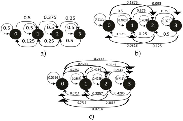
To analyze the convergence and the stability of the Ehrenfest process, we implement a numerical example for four balls and $\beta =1/2$. We focus our attention on the following issues: how the probabilistic terms in the rows are transformed and how the matrix evolves after N steps. The following matrix expressions show the resulting stochastic matrix after 1, 2, and 25 steps.

$$\begin{array}{l}E=\left(\begin{array}{cccc}0.5000& 0.5000& 0& 0\\ 0.1250& 0.5000& 0.3750& 0\\ 0& 0.2500& 0.5000& 0.2500\\ 0& 0& 0.5000& 0.5000\end{array}\right),E^2=\left(\begin{array}{cccc}0.3125& 0.5000& 0.1875& 0\\ 0.1250& 0.4063& 0.3750& 0.0938\\ 0.0313& 0.2500& 0.4688& 0.2500\\ 0& 0.1250& 0.5000& 0.3750\end{array}\right),\\ \cdots ,\\ E^{25}=\left(\begin{array}{cccc}0.0714& 0.2857& 0.4286& 0.2143\\ 0.0714& 0.2857& 0.4286& 0.2143\\ 0.0714& 0.2857& 0.4286& 0.2143\\ 0.0714& 0.2857& 0.4286& 0.2143\end{array}\right).\end{array}$$E14

From the last matrix expression, we can identify that all elements in each column have the same value; consequently, all rows have the same entropy value that corresponds to the final equilibrium state [12]. The structure of Eq. (14) shows that the product of a row in the arbitrary random vector with an N-step stochastic matrix reproduces the matrix row. This represents the equilibrium of the process, and a surprising result is that the final entropy does not depend on the initial random vector. From this entropy value, it is possible to deduce some generic features. For example, the maximum entanglement between the probabilistic values in the n-step random matrix. This can be obtained by analyzing the digraphs evolution shown in Figure 1. The entanglement features carry information on the evolution of the different probability states between the nodes. This analysis is contained in the entropy value evolution.

Figure 1.

Depicture of the stochastic matrix process corresponding to Eq. (14). (a) Digraph associated with the initial stochastic matrix. (b) Digraph for $E^2$. (c) Digraph for $E^{25}$, showing when the process reaches a standard configuration.

Finally, we remark that the changes in the assigned probability values in the initial stochastic matrix imply the modification of the connectivity between states. This information becomes evident in Table 1; however, all the nodes acquire invariant connectivity between the probabilistic states obtained from the n-step probabilistic matrix.

	0	1	2	3
0	0.0714	0.2857	0.4286	0.2143
1	0.0714	0.2857	0.4286	0.2143
2	0.0714	0.2857	0.4286	0.2143
3	0.0714	0.2857	0.4286	0.2143

Table 1.

Numerical representation of the digraph shown in Figure 1(c).

5. Generation of Ehrenfest optical modes

The purpose of this section is to implement an Markovian Ehrenfest process in the optical context. To perform this, we define an optical mode as an exact solution to the Helmholtz equation. The mathematical expression is of the form [13]:

$$\varphi \left(x,y,z\right)=f\left(x,y\right)exp\left(\mathit{i\beta z}\right),$$E15

where the function f(x, y) must satisfy the eigenvalue equation

$${\nabla }_{\perp }^{2}f\left(x,y\right)+K^{2}f\left(x,y\right)={\beta }^{2}f\left(x,y\right),$$E16

the transversal profile f(x, y) remains invariant when it is propagating along the z coordinate. For mathematical convenience, we solve Eq. (16) by using polar coordinates, allowing us to identify the solutions as a set of Bessel functions of integer order. The optical modes are given by

$$\left\{e^{\mathit{i\beta z}}{J}_n\left(2\mathit{\pi rd}\right)e^{\mathit{in\theta }}\right\}n=0,\pm 1,\pm 2,\dots .$$E17

It should be noted that all of the modes have the same phase value that describes the mode propagation along the z coordinate. This is a condition for all the modes present diffraction-free features. We will use the representation to generate a tandem array of optical modes following a Markovian chain, i.e., we engineer a stochastical mode that locally presents diffraction-free features. An important case occurs when a set of integer-order Bessel modes are selected following a Markov chain type process.

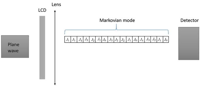
Eq. (17) can be matched with the box model of the Ehrenfest process described in the previous section. By replacing the label in each ball by $J_0,J_1,\dots ,J_n$ the evolution of initial state is described $x_0=\left(a_0,\dots ,a_n\right).$ This vector corresponds to the coordinates representing the appearance of the mode with the following interpretation: Assuming that the process has time duration T, divided by n subintervals of length $\mathrm{\Delta }T.$ In each subinterval, a Bessel mode of integer order is selected. Thus, the optical field consists of a succession of mode-type chains where the occurrence of the ith Bessel mode is $n{\alpha }_i$. With this interpretation, the optical field assumes the structure shown in Figure 2. A liquid crystal display (LCD) is implemented to generate the boundary condition that consists of an annular slit angularly modulated for synthesizing the corresponding Bessel mode [13, 14]. The chain structure corresponds to an Ehrenfest mode.

Figure 2.

To generate the Bessel modes, an LCD is illuminated containing an annular slit with time-dependent angular modulation with a coherent plane wave linearly polarized.

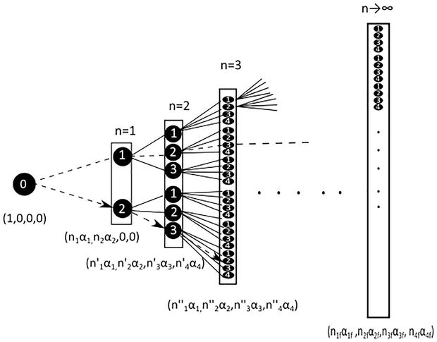
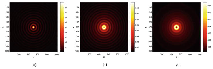
To get an understanding of the evolution of the Markovian mode, it is convenient to describe a tree graph, shown in Figure 3. The dotted line represents the sequence $\left({\mathrm{J}}_0-{\mathrm{J}}_0-{\mathrm{J}}_1-{\mathrm{J}}_2\dots \right),$ and the dotted arrowed line represents $\left({\mathrm{J}}_0-{\mathrm{J}}_1-{\mathrm{J}}_2-{\mathrm{J}}_1\dots \right).$ From this representation, time-structured modes are generated, and all of them must exhibit the same irradiance mean when the equilibrium is reached. In the early steps, the corresponding modes display different irradiance values as shown in Figure 4 obtained with commercial software.

Figure 3.

Sketch of the entanglement between states as “n” grows; during this evolution, it is possible to visualize that the probability density is distributed between the accessible states.

Figure 4.

The mean irradiance after N-steps for an Ehrenfest-type process. (a) Represents the initial state associated with a $J_0$ Bessel mode. The initial probability vector is (1, 0, 0, 0). (b) Mean irradiance after 2-steps, and the probability vector is (1/2, 1/2, 0, 0). (c) Mean irradiance after 25-steps, the probability vector is (0.0714, 0.2857, 0.4286, 0.2143). It must be noted that this last vector corresponds to a row for the stabilized N-step stochastic matrix. The expression for the mean irradiance can be related to the probability vector as $I{=}^{\left(N\right)}n\left(P_0^2{J}_0^2+P_1^2{J}_1^2+P_2^2{J}_2^2\right),$ where ${}^{\left(N\right)}{\mathit{nP}}_i$ is the occurrence number for the irradiance of each mode.

The Ehrenfest mode consists of a sequence of Bessel modes of integer order where each sequence appears according to a certain probability value. The state starts with a zero-order Bessel beam, whose irradiance is shown in Figure 4–a, which evolves following the chain and after three steps, the initial vector evolves toward the vector whose irradiance is given by ${\alpha }_0^{\left(2\right)}{J}_0^2+{\alpha }_1^{\left(2\right)}{J}_1^2+{\alpha }_2^{\left(2\right)}{J}_2^2$. When the experiment is performed n-times, the number of occurrences of each element of the basis can be obtained from the transformed random vector. The mean of irradiance after three steps is shown in Figure 4–b. When the number of steps increases, the chain is stabilized and the irradiance means distribution is shown in Figure 4–c. The global optical fields were analyzed once the equilibrium was reached. The mean irradiance distribution presents diffraction-free features. The latter is easily understood since the irradiance associated with each mode is non-depending on the z-coordinate. However, locally these fields follow a sequence of optical modes according to the Markov chain selected. The resulting optical mode consists of a sequence of time-changing blocks that do not follow a stationary process. For this reason, the mode is characterized using the entropy models in the following section.

6. Entropy, purity, and interference between Markovian modes

Using the fact that a Markovian process is associated with a stochastic matrix, some generic properties through entropy description can be identified allowing the study of the mode’s structural features. The calculus of the Von Neumann entropy is proposed [15] in order to obtain a reference to compare the entropy value from the N-step stochastic matrix. The entropy is calculated from the principal diagonal elements, and we remark that the resulting value acts as a reference value for the different entropy measurements obtained from the elements of the rows in the N-steps resulting matrix; also as the entropy obtained in the secondary diagonal, this last value contains information about the correlation among the constitutive modes [16]. By comparing these entropy values, it can be deduced how the correlation function evolves, which allows us to understand the irradiance distribution as a function of N, which represents the number of applications of the initial stochastic matrix. The Von Neumann entropy is defined as

$$S_c=-\mathrm{Tr}D\left(E^N{\mathit{LnE}}^N\right),$$E18

where Tr denotes the trace of stochastic matrix $E^N\mathrm{Ln}\left(E^N\right).$ It should be noted that this type of entropy contains information for the irradiance distribution. However, we need to describe the entanglement among the elements of the basis. This description can be obtained by proposing the correlation entropy calculus as an ansatz using the elements in the secondary diagonal. This entropy takes the following form:

$$S_v=-\mathrm{Tr}\left(E^N\mathrm{Ln}{E}^N\right),$$E19

where TrD denotes the trace of the secondary diagonal. Furthermore, a good method for describing the mode structure is applied by calculating the difference of the entropy values, which is expressed as

$$\mathrm{\Delta }S=S_c-S_v.$$E20

From this last definition, it can be easily proved that the correlation entropy is always lower-bounded by the Von Neumann entropy $S_c,\dots S_v.$ To compare the entropy values, each diagonal needs to satisfy the normalization condition. From Eq. (20), certain interesting cases can be identified. The limit case occurs when $\mathrm{\Delta }S=0.$ Its physical meaning is that all irradiance events involved during the process participate in the global irradiance distribution, another case occurs when $\mathrm{\Delta }S=S.$ There is no interaction among the elements of the basis; thus, they are statistically independent. However, this case is not permitted in the Markov chain-type Ehrenfest process. Finally, another entropy measurement can be obtained from the qth-row elements, expressed as

$${}_q{S}_f=-\sum _i{\alpha }_{\mathit{iq}}\mathit{Ln}\left({\alpha }_{\mathit{iq}}\right),$$E21

where ${\alpha }_{\mathit{iq}}$ denotes the elements in the qth row and satisfies ${\sum }_i{\alpha }_{\mathit{iq}}=1$ for $q=\mathrm{0,1,2},\dots ,n.$ From this set of entropy values, an order relationship is easily identified, e.g.,

$$S_q<S_2=S_4<S_5<\dots ,$$E22

this means that a qth-Bessel mode appears in a principal manner, followed by the second-order Bessel mode that appears in the same proportion as the fourth-order Bessel modes, and so on. From this order relationship, we can associate a purity measurement to the Ehrenfest mode [17] as follows:

$$P_q=1-\frac{S_q^{\left(n\right)}}{{\sum }_{l=0}^N{S}_i^{\left(n\right)}},$$E23

which determines the similitude of the Markovian mode with the $J_q$ mode because ${\sum }_{q=0}^n{P}_q=1.$ The entropy values for the Ehrenfest mode are given by $S_v=S_c=0.5383$. The equality indicates that the process reaches an equilibrium condition. In addition, all of the rows have the same entropy value. Consequently, from the purity definition, it can be deduced that the resulting mode is the same for each element of the basis. This result is expected because the Ehrenfest process describes the conditions to reach an equilibrium system. Consequently, once the equilibrium condition is reached and as a result of the isotropy of the process, all the elements of the basis in the resulting random vector appear in the same proportion. The purity concept describes the times each element appears in a given mode.

7. Conclusions

We described the synthesis of Markovian optical modes that have diffraction-free features. The type of optical field was obtained by means of a tandem array or chain of Bessel modes. The chain evolves following a Markovian process. We present an example for a Markov-chain process type Ehrenfest. This type of process is very important since the theoretical point of view because it is close related to the thermodynamical process establishing a geometrical point of view for the entropy evolution. The optical mode reaches an equilibrium condition, which can be deduced from the N-step stochastical matrix. This condition is identified when the random rows of the matrix have the same entropy value. Using the entropy values we define the purity of the mode, and this definition allows to compare the similitude of the Markovian mode with a single Bessel mode. A very important result of the chapter is that changing the probabilistic values in the Markovian matrix all the Ehrenfest matrixes reaches the same final configuration; however, the number of steps is different. This property corresponds to hysteresis effect. These features allow to implement inverse processes in particular offering the possibility to generate Markovian holographic process. In the optical context, the Markovian optical mode can be used as illumination beam to generate random diffraction also as it can be implemented to generate tunable optical tweezers inducing tunable spectroscopy features [18, 19, 20, 21]. Other immediate applications are cryptographic transference information, entanglement of arbitrary optical fields, and self-healing analysis [22, 23, 24, 25, 26, 27].

References

1.Kanseri B, Singh HK. Development and characterization of a source having tunable partial spatial coherence and polarization features. Optik. 2020;206:163747
2.Tang X, Xu X, Yan Z. Tunable optical tweezers by dynamically sculpting the phase profiles of light. Applied Physics Express. 2021;14:022009
3.Shoji T, Tsuboi Y. Plasmonic optical tweezers toward molecular manipulation: Tailoring Plasmonic nanostructure, light source, and resonant trapping. Journal of Physical Chemistry Letters. 2014;5:2957-2967
4.Li A et al. Enabling Technology in High-Baud-Rate Coherent Optical Communication Systems. IEEE Access. 2020;8:111318-111329
5.Korotkova O, Wolf E. Changes in the state of polarization of a random electromagnetic beam on propagation. Optics Communications. 2005;246:35-43
6.Tervo J, Setl T, Friberg AT. Theory of partially coherent electromagnetic fields in the spacefrequency domain. Journal of the Optical Society of America A. 2004;21:2205-2215
7.Gbur G. Partially coherent beam propagation in atmospheric turbulence. Journal of the Optical Society of America A. 2014;31:2038-2045
8.Mandel L, Wolf E. Optical Coherence and Quantum Optics. New York, NY, USA: Cambridge University Press; 1995
9.Hoel SPH, Stone C. Introduction to Sthochastic Processes. Boston, USA: Houghton Mifflin; 1972
10.Coleman R. Stochastic Processes, Problem Solvers. Netherlands: Springer; 1974
11.Costantini D, Garibaldi U. The ehrenfest fleas: From model to theory. Synthese. 2004;139:107142
12.Chen Y-P. Which design is better? Ehrenfest urn versus biased coin. Advances in Applied Probability. 2000;32:738749
13.Durnin J. Exact solutions for nondiffracting beams. i. the scalar theory. Journal of the Optical Society of America A. 1987;4:651654
14.Martinez-Niconoff G, Martinez-Vara P, Andres-Zarate E, Silva-Barranco J, Munoz-Lopez J. Synthesis of sources with Markovian features. Journal of the European Optical Society Rapid Publications. 2013;8:13005(1-7)
15.Barakat R, Brosseau C. Von neumann entropy of n interacting pencils of radiation. Journal of the Optical Society of America A. 1993;10:529532
16.Selvamuthu D, Di Crescenzo A, Giorno V, Nobile A. A continuous-time ehrenfest model with catastrophes and its jump-diffusion approximation. Journal of Statistical Physics. 2015;161:326345
17.Picozzi A. Entropy and degree of polarization for nonlinear optical waves. Optics Letters. 2004;29:16531655
18.Pang Y, Gordon R. Optical trapping of a single protein. Nano Letters. 2012;12:402-406
19.Cao T, Qiu Y. Lateral sorting of chiral nanoparticles using Fano-enhanced chiral force in visible region. Nanoscale. 2018;10:566-574
20.Hester B, Campbell GK, Lpez-Mariscal C, Filgueira CL, Huschka R, Halas NJ, et al. Tunable optical tweezers for wavelength-dependent measurements. The Review of Scientific Instruments. 2012;83:043114
21.Teeka C, Jalil MA, Yupapin PP, Ali J. Novel tunable dynamic tweezers using dark-bright soliton collision control in an optical add/drop filter. IEEE Transactions on Nanobioscience. 2010;9:258-262
22.Sapozhnikov O. An exact solution to the helmholtz equation for a quasi-gaussian beam in the form of a superposition of two sources and sinks with complex coordinates. Acoustical Physics. 2012;58:4147
24.Barnett SM, Phoenix SJD. Entropy as a measure of quantum optical correlation. Physical Review A. 1989;40:2404-2409
25.Jones PH, Marag OM, Volpe G. Optical Tweezers: Principles and Applications. United Kingdom, UK: Cambridge University Press; 2015
26.Wang F, Chen Y, Lina G, Liu L, Cai Y. Complex gaussian representations of partially coherent beams with nonconventional degrees of coherence. Journal of the Optical Society of America A. 2017;34:1824-1829
27.Janousek J, Morizur J-F, Treps N, Lam PK, Harb C, Bachor H-A. Optical entanglement of co-propagating modes. Nature Photonics. 2009;3:399-402
Written By
Patricia Martinez Vara, Juan Carlos Atenco Cuautle, Elizabeth Saldivia Gomez and Gabriel Martinez Niconoff
Submitted: 21 December 2022Reviewed: 24 February 2023Published: 10 August 2023
Open access peer-reviewed chapter