Hidden Markov Models for Pattern Recognition

Abstract

Hidden Markov Models (HMMs) are the most popular recognition algorithm for pattern recognition. Hidden Markov Models are mathematical representations of the stochastic process, which produces a series of observations based on previously stored data. The statistical approach in HMMs has many benefits, including a robust mathematical foundation, potent learning and decoding techniques, effective sequence handling abilities, and flexible topology for syntax and statistical phonology. The drawbacks stem from the poor model discrimination and irrational assumptions required to build the HMMs theory, specifically the independence of the subsequent feature frames (i.e., input vectors) and the first-order Markov process. The developed algorithms in the HMM-based statistical framework are robust and effective in real-time scenarios. Furthermore, Hidden Markov Models are frequently used in real-world applications to implement gesture recognition and comprehension systems. Every state of the model can only observe one symbol in the Markov chain. In contrast, every state in the topology of a Hidden Markov Model can see one symbol emerging from a particular gesture. The matrix representing the observation probability distribution contains the likelihood of observing a symbol in each state. As an illustration, the probability that a symbol will emit is determined by its observation probability in the first state. In the recognition task, the emission distribution is another name for the observation probability distribution. For the following reasons, HMM states are also referred to as hidden. First, choosing to emit a symbol denotes the second process. Second, an HMM’s emitter only releases the observed symbol. Finally, since the current states are derived from the previous states, the emitting states are unknown. HMMs are well-known and more flexible in the field of gesture recognition because of their stochastic nature.

1. Introduction

One of the greatest methods for pattern recognition is HMM since it can deal with the issues caused by spatiotemporal variability [1, 2, 3, 4]. Additionally, HMMs have been effectively used in the classification of gestures, speech, modeling of proteins, etc. [2, 5, 6, 7, 8]. Because segmentation and recognition are tuned concurrently during recognition using HMMs, the use of HMMs increases the effectiveness of recognition-based segmentation. The two categories of gesture are communicative gestures (also known as key gestures or meaningful gestures) and noncommunicative gestures (i.e., garbage gesture or transition gesture) [9, 10, 11, 12]. In other words, as indicated in Figure 1, a natural gesture comprises three phases: pre-, key-, and post-gesture. The key gesture may be described as a hand trajectory component that has clear human significance. While pre- and post-gestures signify inadvertent motion utilized to integrate important gestures (Figure 1).

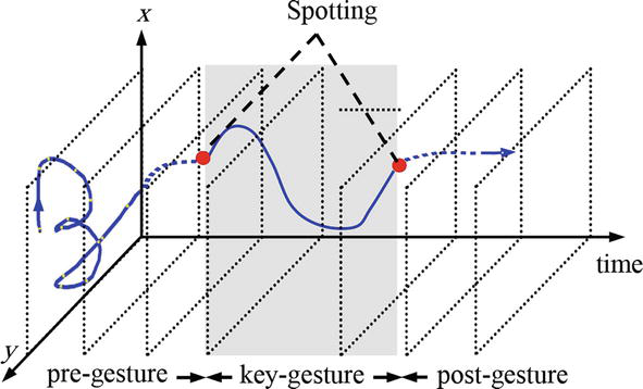
Figure 1.

Three main phases for the trajectory for spotting meaningful gestures.

A method to detect American Sign Language was developed by Vogler and Metaxas [13], using HMMs and three video cameras (ASL). To extract 3D characteristics of the user’s hand and arm, they employed an electromagnetic tracking device. Two trials using 99 texts and 22 signals to test their method were conducted. Both single signals and full phrases were used in the trials. For isolated signs and continuous phrases, their system has obtained recognition rates of 94.5 and 84.5%, respectively. A data collection of 40 signs was used by Starner et al. [5] to present two HMM-based algorithms. While the second technique embeds the camera on the user’s headgear, the first system depends on the camera’s presence on a desk. According to hand shapes as extracted characteristics, the trials have been run on continuous data collection. The systems accuracy rates for the first and second systems were 92 and 98%, respectively.

A German Sign Language (GSL) recognition system based on HMMs was presented by Bauer and Kraiss [14] and uses colored gloves. Both continuous and isolated indicators have been used to test the system. Subunit HMMs were employed in their system to identify isolated signs and carry out the spotting signs. The system detected spotted hand signals with an accuracy of 92.5% for 100 isolated signs, according to the findings of the experiment.

For French Sign Language (FSL), Braffort [15] presented a recognition method that classified signs into communicative, noncommunicative, and variable signals. In order to extract information like hand position and appearance, a colored glove was utilized. These features were then used to generate HMM codewords. The studies followed classifiers; one was used to identify communicative signs, and the other to identify both noncommunicative and variable indicators. For a repertoire of seven signs, their method achieves a 96% recognition rate.

The approach used by Lee and Kim [6] is regarded as one of the pioneering examples of distinct modeling that deals with transition gestures. Regardless of the hand morphologies, this approach has been utilized to handle 2D hand trajectory (also known as gesture trajectory). The disadvantage of this technique is that while merging two states, the quantity of samples is not taken into account.

The Hierarchical Activity Segmentation (HAS) method was proposed by Kahol et al. [16, 17]. The HAS algorithm dynamically represented human anatomy using layers of hierarchy. In addition to making several tries to segment a complicated human motion sequence, this algorithm has also taken low-level motion factors into account to distinguish up-bottom motions (e.g., dancing). There were two primary phases that the mechanism of this procedure went through. Three cues were used in the first step to identify the boundaries of potential gestures, and they were then applied in the second step to a naive Bayesian classifier for boundary detection of the right gesture. Individual gesture patterns were analyzed in 3D using coupled HMMs (cHMMs) in order to identify dance sequences. Unlike other studies, which are only interested in key gesture spotting, this method takes into account all transition gestures in person motions. The transition gestures are explicitly modeled in order to identify key gestures precisely. In summary, HMMs effectively model the spatiotemporal aspects of gestures and can manage non-gesture patterns.

The remainder of the chapter is organized as next. Section 2 explores an overview of the Hidden Markov Model. Section 3 conducts hand gesture recognition application and Section 4 provides the concluding remarks.

2. Hidden Markov model

The most popular method for gesture recognition algorithms is Hidden Markov Models (HMMs) [1, 18, 19, 20]. HMMs are mathematical models of the stochastic process and observations, which should be estimated, using a well-defined approach based on previously stored information. The statistical approach in HMMs has numerous benefits as a strong mathematical framework, effective learning and decoding techniques, the ability to handle sequences well, and flexible topology for the statistical syntax. HMMs are a viable option for modeling dynamic gestures since they are time-varying processes that exhibit statistical variation and are frequently employed in practice to put gesture recognition and comprehension systems into place.

Every state in the Markov chain can only see one symbol, whereas the architecture of HMMs allows for more observation, every state can see one sign emerging from a different gesture. The likelihood of finding a symbol for each state is contained in the observation probability distribution matrix. For instance, the probability of observing a symbol in the state $s_1$ is equivalent to the probability of the symbol emitting. Furthermore, HMMs states are called hidden because of (1) Choosing to observe a symbol denotes the execution of the second process; (2) an HMM emitter only emits the symbol that has been chosen to be seen; and (3) the emitting states are unknown since the current states are derived from the prior states. Due to their stochastic character, HMMs are more adaptable and well-known in the field of gesture recognition.

2.1 Elements of HMMs

HMMs can be expressed with $\lambda =\left(A,B,\pi \right)$ and are defined by the following parameters [1, 21, 22, 23];

• The group of states $\mathrm{S}=\left\{s_1,s_2,\dots ,s_N\right\}$. $N$ express the number of states in the technique.

• For each state $\pi$, an initial probability distribution that;

$${\pi }_i=P\left(s_i\right),1\le j\le N$$E1

• An N-by-N transition matrix $\mathrm{A}=\left\{a_{\mathit{ij}}\right\}$, which defined by;

$$a_{\mathit{ij}}=P\left(s_j|s_i\right),1\le i,j\le N$$E2

where $a_{\mathit{ij}}$ is the likelihood that state $s_i$ at time $t$ will change to state $s_j$ at time $t+1$. since the probabilities of changing from one state to another are represented by the entries in each row of matrix A their sum must be equal to 1.

$$\sum _j{a}_{\mathit{ij}}=1$$E3

• The potential observations list $O=\left\{o_1,o_2,\dots ,o_T\right\}$ in which T is the gesture path length.

• The group of symbols $V=\left\{v_1,v_2,\dots ,v_M\right\}$,

where $M$ denotes the different observation symbols for each state (Size of code word).

An N-by-M observation matrix $B=\left\{b_j\left(m\right)\right\}$, where

$$b_j\left(m\right)=P\left(v_m|s_j\right),1\le j\le N,1\le m\le M$$E4

$$\sum _m{b}_j\left(m\right)=1$$E5

where $b_j\left(m\right)$ represents the probability that symbol $v_m$ would be emitted at state $s_j$. For the same obvious reason, the total of each row’s elements in matrix B must equal 1.

Two model parameters ($N$ and $M$) make up a comprehensive specification of the HMMs. It also contains the three probabilistic parameters $A$, $B$, and $\pi$ as well as the observation symbols. Thus, the following is a compact notation for HMM:

$$\lambda =P\left(\pi ,A,B\right)$$E6

Here, $\lambda$ refers to the model’s set of parameters.

2.2 HMMs problems

Mathematically, three variables govern the application of HMMs. These elements are topologies, the chosen emission features, and the probabilities of their observations. The observation job informs the feature choices. Moreover, there are three primary problems that must be resolved to effectively use transition probabilities in practical applications for real-world applications. They are:

• Evaluation problem: How to determine the probability of the observed sequence given the observation sequence $O$‘s model parameter and the model parameter $\lambda$ (i.e., $P\left(O|\lambda \right)$)?

• Decoding problem: How to choose the most efficient route $\lambda$ that generates $O=\left\{o_1,o_2,\dots ,o_T\right\}$ with maximum probability for observation sequence $O$ and model parameter $\lambda$,

• Estimation problem: How to change or update the model $\lambda =P\left(\pi ,A,B\right)$ to generate $O=\left\{o_1,o_2,\dots ,o_T\right\}$ with largest probability? for observation sequence $O$.

2.2.1 Evaluation problem

The simple way is to calculate $P\left(O|\lambda \right)$ by counting all conceivable state sequences $s$ of length $T$ and calculating the corresponding probability $P\left(O|s_1,s_2,\dots ,s_t\right)$ for given observation sequence $O$ and model parameter $\lambda$. Assume that the definition of the forward chain is equal to the probability of the partial observation sequence $O=o_1,o_2,\dots ,o_t$ at state $s_i$ equals the definition of the forward variable $\mathit{\alpha t}\left(i\right)$ (Figure 2) [1]. Therefore,

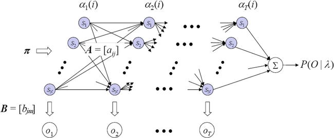
Figure 2.

Forward algorithm for trellis diagram.

$${\alpha }_t\left(i\right)=P\left(o_1,o_2,\dots ,o_t,s_i|\lambda \right)$$E7

Using the following recursive relation, the computation of all forward variables is simple $\alpha$’s

$${\alpha }_{t+1}\left(j\right)=\sum _{i=1}^N{\alpha }_t\left(i\right)\cdot a_{\mathit{ij}}\cdot b_j\left(o_{t+1}\right),1\le j\le N,1\le t\le T-1$$E8

where the $\alpha$ values are calculated as follows:

$${\alpha }_1\left(j\right)={\pi }_j\cdot b_j\left(o_1\right),1\le j\le N$$E9

Therefore, the required probability $P\left(O|\lambda \right)$ with the terminated procedure at $T$ is provided by:

$$P\left(O|\lambda \right)=\sum _{i=1}^N{\alpha }_T\left(i\right)$$E10

The probability of the partial observation sequence is similar $o_{t+1},o_{t+2},\dots ,o_T$ at the state $s_i$ for backward variable ${\beta }_t\left(i\right)$ is defined as:

$${\beta }_t\left(i\right)=P\left(o_{t+1},o_{t+2},\dots ,o_T,s_i|\lambda \right)$$E11

Moreover, compute the recursive relationship ${\beta }_t\left(i\right)$ for calculations of $\alpha$‘s as follows:

$${\beta }_t\left(i\right)=\sum _{j=1}^N{\beta }_{t+1}\left(j\right)\cdot a_{\mathit{ij}}\cdot b_j\left(o_{t+1}\right),1\le i\le N,1\le t\le T-1$$E12

Then,

$${\beta }_T\left(i\right)=1,1\le i\le N$$E13

Hence, for state $s_i$ at time $t$, the multiplication of $\beta$ and $\alpha$ is calculated as follows:

$${\alpha }_t\left(i\right)\cdot {\beta }_t\left(i\right)=P\left(O,s_i|\lambda \right),1\le i\le N,1\le t\le T$$E14

This estimate offers a different calculation $P\left(O|\lambda \right)$ using both forward $\alpha$‘s and backward $\beta$‘s parameters as in (Eq. (15)).

$$P\left(O|\lambda \right)=\sum _{i=1}^N{\alpha }_t\left(i\right)\cdot {\beta }_t\left(i\right)$$E15

Finally, the prior equation is crucial and more precise in predicting the formulas required for gradient-based training.

2.2.2 Decoding issue

To explain the precise state sequence that produces the observations $O=o_1,o_2,\dots ,o_t$ with model parameter $\lambda =\left(A,B,\pi \right)$ and maximum probability is the incentive for solving the decoding problem. Therefore, the Viterbi algorithm which is applied to find the sequence of most likely hidden states to emit the sequence of observed events is employed as in Figure 3 [20].

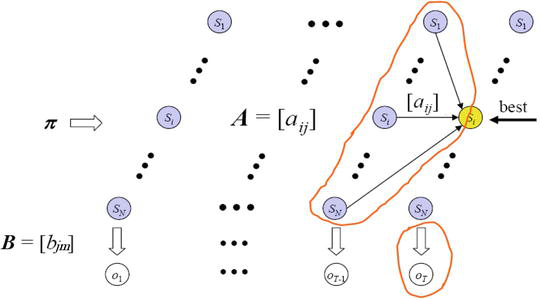
Figure 3.

Forward algorithm for trellis diagram with ${\delta }_t\left(j\right)$ of largest probability of arriving in state$j$ at time $t$.

The Viterbi path is a set of hidden states. The forward variable ${\alpha }_t\left(i\right)$ is implemented similarly to the Viterbi algorithm. During the recursion stage, the maximize over the preceding states makes a difference. An auxiliary variable to make computation easier is defined as follows:

$${\delta }_t\left(j\right)=max\left\{P\left(o_1,o_2,\dots ,o_t,s_1,s_2,\dots ,s_t|\lambda \right)\right\}$$E16

To demonstrate how the Viterbi algorithm works, the following steps are used:

• Step1 (Initialization): $\mathit{\text{for}}1\le i\le N,$

  (a) ${\delta }_1\left(i\right)={\pi }_i\cdot b_i\left(o_1\right)$

  (b) ${\varphi }_1\left(i\right)=0$

• Step2 (Recursion): $\mathit{\text{for}}2\le t\le T,1\le j\le N,$

  (a) ${\delta }_t\left(j\right)=\underset{i}{max}\left[{\delta }_{t-1}\left(i\right)\cdot a_{\mathit{ij}}\right]\cdot b_j\left(o_t\right)$

  (b) ${\varphi }_t\left(j\right)=arg\underset{i}{max}\left[{\delta }_{t-1}\left(i\right)\cdot a_{\mathit{ij}}\right]$

• Step3 (Termination):

  (a) $p^{\ast }=\underset{i}{max}\left[{\delta }_T\left(i\right)\right]$

  (b) $q_T^{\ast }=\mathit{arg}\underset{i}{max}\left[{\delta }_T\left(i\right)\right]$

• Step4 (Reconstruction): $\mathit{\text{for}}t=T-1,T-2,\dots ,1$

$$q_t^{\ast }={\varphi }_{t+1}\left(q_{t+1}^{\ast }\right)$$

The resulted optimal states sequence and tate optimized likelihood function is $q_1^{\ast },q_2^{\ast },\dots ,q_T^{\ast }$. ${\varphi }_t\left(j\right)$ indicates the state index j at time t, and $p^{\ast }$.

2.2.3 Estimation problem

The system’s effectiveness is greatly impacted by the training procedure. A HMM is trained by modifying its model parameters to get the best description for the observation sequence $O_{\mathit{\text{train}}}$. There is currently no analytical method for optimizing HMMs parameters to optimize the likelihood of observed sequences from the training data set [1]. Instead, the Baum-Welch (BW) method is employed to complete the training procedure, so that $\lambda =\left(A,B,\pi \right)$ is optimized with maximum likelihood $P\left(O|\lambda \right)$ [24]. BW is a generalized expectation maximization procedure that is calculated using variables that are both forward and backward [25]. Moreover, BW algorithm uses a number of iterations for the observation sequence to optimize HMMs parameters. BW determines the posterior mode estimate and the maximum likelihood estimation for the HMMs parameters $\left(A,B,\pi \right)$ given a series of observation sequences $o_{\mathit{\text{train}}}\in O$.

To demonstrate how the BW algorithm works, two auxiliary variables are defined. The probability of traveling along an arc $i$ at time $t$ to state $j$ at time $t+1$ (Figure 4) is as follows:

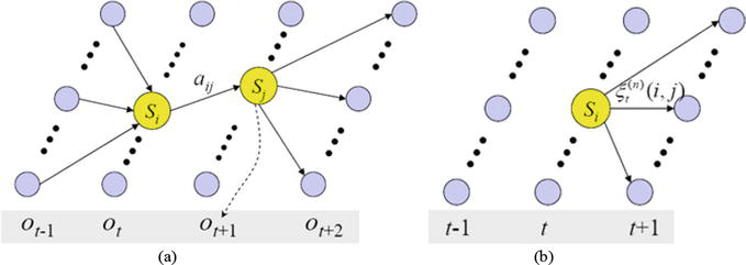
Figure 4.

Trellis diagram learning method according to Baum-Welch. (a) the likelihood of making the journey from state $i$ to state $j$. (b) the likelihood that state $i$ at time $t$.

$${\xi }_t\left(i,j\right)=P\left(s_i\mathit{at}t,s_j\mathit{at}t+1|O,\lambda \right)$$E17

where the transition probability is representing by $\xi$ and Eq. (17) becomes as:

$${\xi }_t\left(i,j\right)=\frac{P\left(s_i\mathit{at}t,s_j\mathit{at}t+1|O,\lambda \right)}{P\left(O|\lambda \right)}$$E18

However, by using forward and backward variables, Eq. (18) becomes:

$${\xi }_t\left(i,j\right)=\frac{{\alpha }_t\left(i\right)\cdot a_{\mathit{ij}}\cdot {\beta }_{t+1}\left(j\right)\cdot b_j\left(o_{t+1}\right)}{{\sum }_{i=1}^N{\sum }_{j=1}^N{\alpha }_t\left(i\right)\cdot a_{\mathit{ij}}\cdot {\beta }_{t+1}\left(j\right)\cdot b_j\left(o_{t+1}\right)}$$E19

The second variable (state probability is defined by;

$${\gamma }_t\left(i\right)=P\left(s_i\mathit{at}t|O,\lambda \right)$$E20

where ${\gamma }_t\left(i\right)$ is the probability of state $i$ at $t$ for given the model parameters and the observation sequence (Figure 4). The following formula Eq. (20) is used to calculate forward and backward variables:

$${\gamma }_t\left(i\right)=\frac{{\alpha }_t\cdot {\beta }_{t+1}}{{\sum }_{i=1}^N{\alpha }_t\cdot {\beta }_{t+1}}$$E21

Therefore, the relationship between ${\gamma }_t\left(i\right)$ and ${\xi }_t\left(i,j\right)$ becomes;

$${\gamma }_t\left(i\right)=\sum _{i=1}^N{\xi }_t\left(i,j\right),1\le i\le N,1\le t\le M$$E22

As a result, BW algorithm modifies the new HMM parameters to have the highest likelihood under the condition $P\left(O|\lambda \right)$. The ${\alpha }^{\prime }$ and ${\beta }^{\prime }$ can be calculated using the recursive equations of (8) and (12) given the initial parameters $\lambda =\left(A,B,\pi \right)$. Eqs. (19) and (22) are used to calculate the auxiliary variables ${\xi }^{\prime }$ and ${\gamma }^{\prime }$, respectively. Moreover, the HMMs parameters are updated as follows:

$${\pi }^{\prime }={\gamma }_1\left(i\right),1\le i\le N,$$E23

$$a_{\mathit{ij}}^{\prime }=\frac{{\sum }_{t=1}^T{\xi }_t\left(i,j\right)}{{\sum }_{t=1}^{T-1}{\gamma }_t\left(i\right)},1\le i\le N,1\le j\le N,$$E24

$$b_j^{\prime }\left(k\right)=\frac{{\sum }_{t=1}^T{\gamma }_t\left(j\right)\cdot {\zeta }_{k,o_t}}{{\sum }_{t=1}^T{\gamma }_t\left(j\right)},1\le i\le N,1\le k\le M,$$E25

where ${\zeta }_{k,o_t}$ is defined as follows:

$${\zeta }_{k,o_t}=\left\{\begin{array}{ll}1& k=o_t\\ 0& \text{otherwise}\end{array}\right.$$E26

2.3 Topologies of HMMs

Because it depends on the training data that is available and the intended model to represent, HMMs topology has a considerable impact on the success of the recognition process. There are three types of HMMs: (1) Fully connected models have positive $a_{\mathit{ij}}$ Ergodic topology coefficients because every state of the model may be reached from any other state. Figure 5 displays topology for $N=4$ the state model.

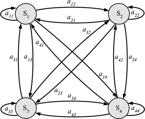
Figure 5.

Ergodic model with four states.

Therefore, the transition among states has become:

$$A=\left(\begin{array}{cccc}{a}_{11}& a_{12}& a_{13}& a_{14}\\ a_{21}& a_{22}& a_{23}& a_{24}\\ a_{31}& a_{32}& a_{33}& a_{34}\\ a_{41}& a_{42}& a_{43}& a_{44}\end{array}\right)$$E27

(2) [18] for the Left–Right model or the Bakis model. According to Figure 6, each state of this model can either proceed to itself or one of the following states. The state transition coefficients of this model have the feature that, for a $N=4$ as illustrated in Figure 6 (which means state transitions whose indexes are lower than the current state are not allowed);

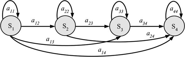
Figure 6.

Left–right model with four states.

$$a_{\mathit{ij}}=0,j<i$$E28

Moreover, the model’s starting state probabilities possess the characteristic;

$${\pi }_i=\left\{\begin{array}{ll}0& i\ne j\\ 1& i=j\end{array}\right.$$E29

where the state sequence must begin from $s_1$ and transition among states of Figure 6 becomes;

$$A=\left(\begin{array}{cccc}{a}_{11}& a_{12}& a_{13}& 0\\ 0& a_{22}& a_{23}& a_{24}\\ 0& 0& a_{33}& a_{34}\\ 0& 0& 0& a_{44}\end{array}\right)$$E30

The transition coefficients, specifically for the final state in a left–right model, are described as follows using the laws of probability:

$$a_{\mathit{NN}}=1,a_{\mathit{Ni}}=0,i<N$$E31

(3) The Left–Right Banded model (LRB) is shown in (7) [21]. The LRB model arranges the states from left to right, and each one has a positive probability of returning to either itself or the one after it. The model’s state transition coefficients exhibit the characteristic;

$$A=\left(\begin{array}{cccc}{a}_{11}& a_{12}& 0& 0\\ 0& a_{22}& a_{23}& 0\\ 0& 0& a_{33}& a_{34}\\ 0& 0& 0& a_{44}\end{array}\right)$$E32

Therefore, in an LRB model, the last state’s and other states’ state transition coefficients are as follows:

$$a_{\mathit{NN}}=1,a_{\mathit{ij}}=0,i<j;j-i\ge 2$$E33

and any HMM parameter with a zero initial value stays zero throughout the estimate procedure. The Left–Right Banded model will thus have a detrimental impact on the process (Figure 7).

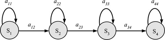
Figure 7.

Left–right banded model with four states.

3. Conducting hand gesture recognition application

A gesture is a spatiotemporal pattern that might be static, dynamic, or both.¹ The term “spatio” refers to locating the hand motion in each frame. To be temporal means to know when a gesture begins and ends. By comparing the identified hand correspondences between subsequent frames, the hand gesture path is determined (Figure 8). It goes without saying that choosing effective features to identify the hand gesture path has a big impact on how well a system performs. The combined features of location, orientation, and velocity with respect to Cartesian systems are used to enhance recognition rates. The HMM codewords are then clustered using K-means. Hand segmentation and feature extraction in computer vision are important steps in developing vision-based hand gesture recognition systems and classification methods for practical applications. Each isolated gesture in our experimental results was based on 60 video sequences, of which 42 were used to train the Baum-Welch algorithm and 18 to test it (i.e., in total, there are 1512 video samples in our database, of which 648 are used for testing). To place a gesture in the appropriate category, the gesture recognition module compares the hand gesture path to a database of reference gestures. The Viterbi algorithm has calculated the greater priority to recognize numbers frame by frame (Figure 9). Our application demonstrated good results to identify isolated integers in real-time implementation. The training and testing procedures are covered in the following subsections.

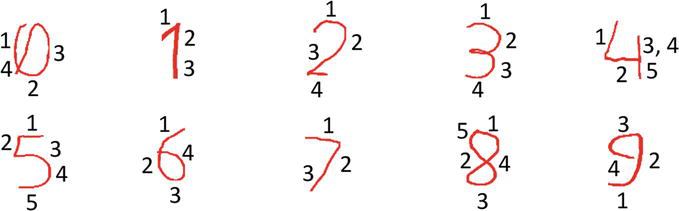
Figure 8.

Hand gesture paths of numbers (0–9) with respect to their segmented parts.

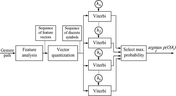
Figure 9.

Block representation of a meaningful gesture recognized by HMMs (Viterbi).

3.1 Model training

The Baum-Welch technique is essential to the proposed system for classifying gestures since it is utilized to train the initialized HMMs parameters $\lambda =\left(A,B,\pi \right)$. To place the tested gesture in the appropriate class, the gesture recognition module compares it to a database of reference gestures. As a result, the Viterbi algorithm recognizes the hand gesture path that maximizes the likelihood of all gesture models. According to Figure 9, the maximal gesture is the one that has the greatest value out of all the gesture models.

3.1.1 Model size

The size of the HMMs must be chosen before the HMMs training process begins. We need how many states, exactly? The complexity of the numerous patterns that will be distinguished by HMMs must be taken into account when estimating the number of states. In other words, when we displayed the graphical pattern, the number of segmented portions was taken into account. The over-fitting² issue arises when there are insufficient training data samples and excessive state numbers are used.

Additionally, using too few states reduces the discrimination capability of HMMs since several segmented parts of a graphical pattern are modeled using the same state. Our gesture recognition method maps each straight-line segment into a single HMM state, which establishes the number of states (Figure 10). We must examine potential patterns to determine how many distinct segments are contained in each pattern in order to represent different graphical patterns. It could be a good idea to employ varying numbers of states in the various HMMs, which were once used to represent various kinds of patterns. For instance, only two states are necessary to represent a graphical pattern “L,” whereas six states are needed to represent a graphical pattern “E,” and four states are needed to represent a graphical pattern “3.”

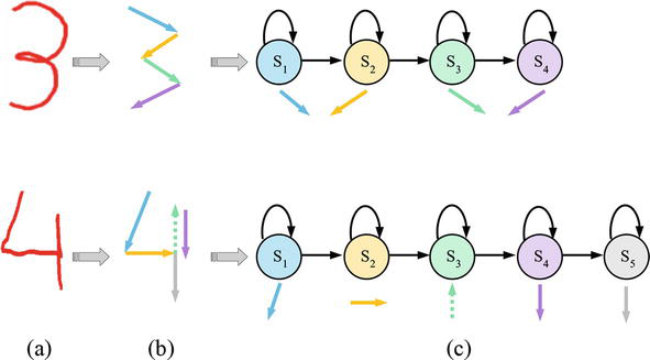
Figure 10.

HMM topologies with a straight-line segment (a) the gesture number derived from the hand motion trajectory (b) the gesture number’s line segment (c) LRB model with segmented line codewords.

3.1.2 Initializing a left: Right banded model

The initial values of each parameter in the HMMs must be set before beginning the iterative Baum-Welch process. The initial model must somehow indicate how we want to represent various model states, and this is the only general need. Nevertheless, depending on the HMMs, this condition has a variety of effects. In reality, the LRB model is taken into account because each state in ergodic topology has more transitions than LR and LRB topologies, making it easy to lose structure data. In contrast, because the LRB topology excludes a backward transition, the state index either rise over time or stays constant. LRB topology is also simpler for training data than LR topology and more constrained, allowing for data-to-model matching [21].

It seems intuitive that a proper initialization of the HMMs $\left(A,B,\pi \right)$ parameters leads to better outcomes. The first parameter is found by applying Eq. (34) to Matrix $A$.

$$A=\left(\begin{array}{ccccc}{a}_{11}& 1-a_{11}& 0& \cdots & 0\\ 0& a_{22}& 1-a_{22}& \cdots & 0\\ ⋮& ⋮& ⋮& \ddots & ⋮\\ 0& 0& 0& \cdots & 1\end{array}\right)$$E34

It is possible to select the transition matrix’s diagonal elements $a_{i}i$ to roughly represent the average state durations $d$ in the following ways:

$$a_{\mathit{ii}}=1-\frac{1}{d}$$E35

and

$$d=\frac{T}{N}$$E36

Such that $T$ denotes the gesture path’s length and $N$ is the number of states.

This is adequate for an automatic training method where state 1 is intended to represent the first part of the training data, state 2 the second part, etc. As a result, the same parameters can be used to initialize all output probability distributions for various states. As a result, the training data are used to determine more accurate output probability parameters for each state in the first iteration of the Baum-Welch algorithm. Due to the discrete nature of HMM states, all members of matrix $B$ are initially set to the same value for each state (Eq. (38)). In the matrix $B$, which consists of $N$-by-$M$ observed symbols, $b_{\mathit{im}}$ denotes the likelihood that symbol $v_m$ would emit in state $i$ (Eq. (4)).

$$b_{\mathit{im}}=\frac{1}{M}$$E37

where $i$, $m$ represent the total number of states and discrete symbols, respectively.

$$B=\left(\begin{array}{cccc}{b}_{11}& b_{12}& \cdots & b_{1M}\\ b_{21}& b_{22}& \cdots & b_{2M}\\ ⋮& ⋮& \ddots & ⋮\\ b_{N1}& b_{N2}& \cdots & b_{\mathit{NM}}\end{array}\right)=\left(\begin{array}{cccc}\frac{1}{M}& \frac{1}{M}& \cdots & \frac{1}{M}\\ \frac{1}{M}& \frac{1}{M}& \cdots & \frac{1}{M}\\ ⋮& ⋮& \ddots & ⋮\\ \frac{1}{M}& \frac{1}{M}& \cdots & \frac{1}{M}\end{array}\right)$$E38

The state can return on its own or merely to the next closest state for each new time sample. Consequently, the $\pi$ initial probability vector should be set up as:

$$\pi ={\left(10\cdots 0\right)}^T$$E39

This will guarantee that we begin from the initial state.

3.1.3 Termination of HMMs learning

The Baum-Welch training algorithm is quite effective. After 5–10 iterations, a satisfactory model is frequently found. The trained model must be flexible enough to faithfully represent an entirely new test sequence after training. The training procedure is repeated until the transition and emission matrices change. If the change is smaller than 0.001, that is, tolerance $\epsilon =0.001$) as indicated in Eq. (40), or if the maximum number of iterations is reached (i.e., 500), the convergence is satisfied.

$$\sum _{i=1}^N\sum _{j=1}^N\mid {\widehat{a}}_{\mathit{ij}}-a_{\mathit{ij}}\mid +\sum _{j=1}^N\sum _{m=1}^M\mid {\widehat{b}}_{\mathit{jm}}-b_{\mathit{jm}}\mid <\epsilon$$E40

The primary purpose of tolerance is to reduce the number of steps the Baum-Welch algorithm needs to take to successfully complete a task. The process is stopped if any one of the next three quantities falls below the tolerance limit. First, a current observation sequence’s log-likelihood ($O$) is generated using the most recent estimates for the values of the transition matrix ($A$) and observation matrix ($B$). Second, a modification in the transition matrix $A$’s normalization. Finally, the observation matrix $B$’s normalization was changed.

Keep in mind that the Baum-Welch algorithm required fewer steps to run before terminating as the level of tolerance increased. In actuality, the maximum number of iterations regulates the maximum number of algorithm execution steps. The termination occurs with a warning if the Baum-Welch algorithm runs for 500 iterations before reaching the chosen tolerance value. If this happens, the algorithm should be allowed to run for a greater maximum number of iterations until it meets the specified tolerance before terminating. The provision of enough training data is typically exceedingly challenging. Because of this, some observations may never occur in the tiny collection of training data, even if we may be aware that they may have happened with some small probability. When a discrete HMM is trained on such data, Baum-Welch will assign a zero observation probability to some of the matrix’s elements. In this situation, a very small nonzero value may be allocated, and the row matrix would need to be renormalized. The matrix representing the transition probabilities might lead to a similar issue. We purposefully assigned several of the transition probability matrix’s entries identically zero values for a left–right banded HMM. After the Baum-Welch training, these elements still have zero values, and they should keep it that way. After completing the training process, it is crucial to adjust the HMMs’ parameters.

3.2 Model testing

The process of classification greatly benefits from the selection of the best HMM topology. The goal of the work is to create HMM topologies with a variety of state numbers in order to select the topology that will produce the best outcomes for an isolated gesture system. An extracted discrete vector features from image sequences are subjected to the application of HMMs with Left–Right Banded (LRB), Left–Right (LR), and Ergodic topologies. These topologies are taken into consideration with a variety of states ranging from 3 to 10. Our gesture recognition system uses the complexity of each gesture number to calculate the number of states by mapping each straight-line segment into a single HMMs state (Figures 8 and 10). For two reasons, the number of states is a significant parameter. First, the over-fitting issue is caused by the use of excessive state numbers when there are not enough training data samples. Second, having too few states reduces the discrimination capacity of HMMs since multiple segmented parts of a graphical pattern are modeled on a single state.

In practice, the LRB model with five states is really used in the gesture recognition system in order to guarantee that all of the states are used. The structure data is easily lost in Ergodic topology since each state has more transitions than in LR and LRB topologies. Completely contrary, the LRB topology avoids a backward transition in which the state index either increases or stays as time goes on. LRB topology is also easier to train on data than LR topology and more constrained in its ability to match data to the model. Additionally, the gesture paths “4” and “5” have the most segmented sections, so using 5 states is taken into consideration to make sure all of these parts are utilized. The recognition ratio is the number of recognized gestures correctly to the number of tested gestures (Eq. (41)).

$$\mathit{\text{Recognition}}\mathit{\text{ratio}}=\frac{\#\mathit{\text{recognized}}\mathit{\text{gestures}}}{\#\mathit{\text{test}}\mathit{\text{gestures}}}\times 100\%$$E41

The BW method is used to train the HMM topologies and the Viterbi algorithm is used to test them. From Figure 11, the LRB performs the best performance, with an average ratio of 97.78% for states ranging from 3 to 10. Additionally, topologies with 4 states in LR and LRB received the greatest recognition. Additionally, compared to LR and Ergodic topologies, LRB topology is always superior. In Figure 11, there is not a significant difference between LRB and LR in terms of outcomes, and the results of the ergodic topology were subpar in comparison to those of LRB and LR topologies. LRB topology with a number of states equal to 5 is typically the best in terms of its impact on gesture recognition in empirical studies.

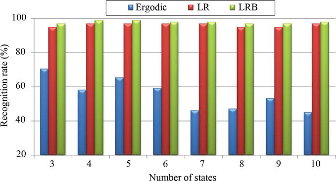
Figure 11.

Results of isolated gesture recognition for three HMMs topologies using states ranging from 3 to 10.

4. Conclusions

The foundational Hidden Markov Model method was discussed in this chapter. HMMs are generative models that put a strong emphasis on modeling the observation in order to compute the conditional probability and specify the joint probability distribution in order to resolve a conditional problem. This study assists in determining the best HMM topology and classification method in terms of outcomes. Furthermore, an application was made on recognizing the gesture of the hand for Arabic numbers from 0 to 9 using the classifier of HMMs in terms of their impact on gesture recognition. In addition, studies and research have been conducted on the effects of HMMs with ergodic, left–right, and left–right banded topologies, as well as varying numbers of states ranging from 3 to 10, on hand gesture recognition. It is concluded that there is not a significant difference between LRB and LR in terms of results and that Ergodic topology performed poorly in comparison to LRB and LR topologies. LRB topology with a total of 5 states is typically the best in terms of its effect on gesture recognition.

Abbreviations

HMMs	Hidden Markov Models
ASL	American Sign Language
GSL	German Sign Language
FSL	French Sign Language
HAS	Hierarchical Activity Segmentation
cHMMs	coupled HMMs
BW	Baum-Welch algorithm
LR	Left–Right model
LRB	Left–Right Banded model

References

- 1.
Rabiner L. A tutorial on hidden Markov models and selected applications in speech recognition. Proceedings of the IEEE. 1989; 77 (2):257-286 - 2.
Wang L, Hasegawa-Johnson M. A DNN-HMM-DNN hybrid model for discovering word-like units from spoken captions and image regions. Interspeech. 2020:1456-1460. DOI: 10.21437/interspeech.2020-1148 - 3.
Wang N, Wang L, Sun Y, Kang H, Zhang D. Three-module modeling for end-to-end spoken language understanding using pre-trained DNN-HMM-based acoustic-phonetic model. Interspeech. 2021:4718-4722. DOI: 10.21437/interspeech.2021-501 - 4.
Amoolya G, Hans A, Lakkavalli V, Durai S. Automatic speech recognition for Tulu language using Gmm-hmm and DNN-HMM techniques. In: 2022 International Conference on Advanced Computing Technologies and Applications (ICACTA). Coimbatore, India: IEEE; 2022. DOI: 10.1109/ICACTA54488.2022.9753319 - 5.
Starner T, Weaver J, Pentland A. Real-time American sign language recognition using desk and wearable computer based video. IEEE Transaction on Pattern Analysis and Machine Intelligence. 1998; 20 (12):1371-1375 - 6.
Lee H, Kim J. An HMM-based threshold model approach for gesture recognition. IEEE Transaction on Pattern Analysis and Machine Intelligence. 1999; 21 (10):961-973 - 7.
Gao W, Fang G, Zhao D, Chen Y. Transition movement models for large vocabulary continuous sign language recognition. In: IEEE International Conference on Automatic Face and Gesture Recognition. Seoul, Korea (South): IEEE; 2004. pp. 553-558 - 8.
Yang J, Pan J, Li J. sEMG-based continuous hand gesture recognition using GMM-HMM and threshold model. In: 2017 IEEE International Conference on Robotics and Biomimetics (ROBIO). Macau, Macao: IEEE; 2017. DOI: 10.1109/ROBIO.2017.8324631 - 9.
Yang H, Park A, Lee S. Gesture spotting and Recognitiomn for human-robot interaction. IEEE Transaction on Robotics. 2007; 23 (2):256-270 - 10.
Kahol X. Gesture segmentation in complex motion sequences. [Master’s thesis] Arizone State University, Tempe, AZ. 2003 - 11.
Elmezain M, Alwateer M, El-Agamy R, Atlam E, Ibrahim H. Forward hand gesture spotting and prediction using HMM-DNN model. Informatics. 2022; 10 :1. DOI: 10.3390/informatics10010001 - 12.
Nguyen N, Phan T, Kim S, Yang H, Lee G. 3D skeletal joints-based hand gesture spotting and classification. Applied Sciences. 2021; 11 :4689. DOI: 10.3390/app11104689 - 13.
Vogler C, Metaxas D. A framework for recognizing the simultaneous aspects of American sign language. Journal of Computer Vision and Image Understanding. 2001; 81 (3):358-384 - 14.
Bauer B, Kraiss K. Video-based sign recognition using self-organizing subunits. In: International Conference on Pattern Recognition. Quebec City, QC, Canada: IEEE; 2002. pp. 434-437 - 15.
Braffort A. ARGo: An architecture for sign language recognition and interpretation. In: International Gesture Workshop Progress in Gestural Interaction. London: IEEE, Springer; 1996. pp. 17-30 - 16.
Kahol K, Tripath P, Panchanthan S. Automated gesture segmentation from dance sequences. In: IEEE International Conference on Automatic Face and Gesture Recognition. Seoul, Korea (South): IEEE; 2004. pp. 883-888 - 17.
Kahol K, Tripath P, Panchanthan S. Documenting motion sequences: Development of a personalized annotation system. IEEE Multimedia Magazine. 2006; 13 (1):35-47 - 18.
Huang X, Ariki Y, Jack M. Hidden Markov Models for Speech Recognition. Taylor & Francis, Ltd.; 1990. DOI: 10.2307/1268779 - 19.
Elmezain M, Al-Hamadi A, Krell G, El-Etriby S, Michaelis B. Gesture recognition for alphabets from hand motion trajectory using hidden Markov models. In: IEEE International Symposium on Signal Processing and Information Technology. Giza, Egypt: IEEE; 2007. pp. 1192-1197 - 20.
Elmezain M, Al-Hamadi A, Appenrodt J, Michaelis B. A hidden Markov model-based isolated and meaningful hand gesture recognition. International Journal of Electrical, Computer, and Systems Engineering. Academia education; 2009; 3 (3):156-163 2070-3813 - 21.
Elmezain M, Al-Hamadi A, Michaelis B. Real-time capable system for hand gesture recognition using hidden Markov models in stereo color image sequences. Journal of WSCG. 2008; 16 (1) ISSN: 1213-6972:65-72 - 22.
Elmezain M, Al-Hamadi A, Appenrodt J, Michaelis B. A hidden Markov model-based isolated and meaningful hand gesture recognition. In: International Conference on Computer Vision, Image and Signal Processing, PWASET. Vol. 31. Academia.edu; 2008. pp. 394-401 - 23.
Elmezain M, Al-Hamadi A, Appenrodt J, Michaelis B. A hidden Markov model-based continuous gesture recognition system for hand motion trajectory. In: International Conference on Pattern Recognition. Tampa, FL, USA: IEEE; 2008. pp. 519-522 - 24.
Baum L, Petrie T, Soules G, Weiss N. A maximization technique occurring in the statistical analysis of probabilistic functions of Markov chains. The Annals of Mathematical Statistics. 1970; 41 (1):164-171 - 25.
Soriano M, Huovinen S, Martinkauppi B, Laaksonen M. Skin detection in video under changing illumination conditions. In: Proceeding International Conference on Pattern Recognition. Barcelona, Spain: IEEE; 2000. pp. 839-842 - 26.
Tetko I, Livingstone D, Luik A. Neural network studies. 1. Comparison of overfitting and overtraining. Journal of Chemical Information and Computer Sciences. 1995; 35 :826-833
Notes
- Gestures are hand motions, while postures are static morphs of the hands.
- When HMMs describe random error rather than the underlying relationship, over-fitting takes place. Potential over-fitting issues depend not only on the quantity and quality of data and parameters, but also on how well the model structure fits with the degree of model error and the nature of the data. When more training does not improve generalization, additional strategies such as regularization, early stopping, cross-validation, and others are utilized to prevent the issue of over-fitting. The reader can seek for additional information with [26].