Definition of Analytical Hierarchy Process and Its Effect on Environmental Decisions in Engineering for Landfill Siting

Abstract

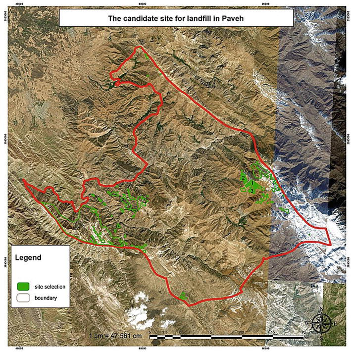
The AHP technique was expanded by Saaty (1980) and called analytic hierarchy process. It is a usual way of multi-criteria decision-making (MCDM) since it was based on theoretical authority. It has a remarkable ability to solve complex problems throughout the decision-making process in any domain. This method, which mirrors human thinking and natural behavior, authorizes the decision-maker to present the interaction between varied criteria in complex and unstructured situations. The AHP method is employed to recognize the consistency of weightings for each criterion, which works by constructing a pairwise comparisons matrix. This chapter aims to examine this method in detail in a tangible example for the field of the environment (landfilling). To obtain this goal, an influential criterion that can affect the decision was considered by using geometric integration in Expert Choice with merging the AHP technique and GIS software. We used governmental regulations, expert’s opinions and previous literature. Paveh is in (Kermanshah) province located in the western part of Iran with 736 km² area. The results show that almost 93% of the study areas are unsuitable for landfill sitting.

1. Introduction

A human being always faces various problems and issues in their life, which they have decide to solve or overcome. Identifying the most appropriate option that can design the path of life and determine its quality [1], swift economic and technological growth over the last fifty years has varied human lives and built modern society confront complex decision-making problems [2]. Multiple criteria decision-making (MCDM) is a significant part of contemporary decision science, aimed at supporting decision-makers faced with various decision criteria and multiple decision alternatives [3]. Considering the problems related to decision-making with multiple criteria, it can be said that due to the lack of standards, the speed and accuracy of decision-making decreases, and decision-making becomes difficult [4]. Such conditions make the decision-making process highly dependent on the decision-maker. To solve this problem or to minimize its side effects, multiple criteria decision-making is designed [5].

Forman and Selly believe that any multi-criteria decision-making system should have the following characteristics [6]:

1. The possibility of formulating the problem and revising.

2. Consider different options.

3. Considering different indicators and criteria.

4. The possibility of using qualitative and quantitative indicators in the decision-making process.

5. Considering different people’s opinions about options and indicators.

6. The possibility of combining judgments.

7. Having a strong theoretical basis.

An excellent and certified weight evaluation method is the analytical hierarchy process (AHP) [7]; this method is one of the most comprehensive processes designed for multi-factor decision-making because with this method, it is possible to formulate the problem hierarchically [8]. In this chapter, we will thoroughly present the AHP method and explain the analysis of this method in an example in the direction of landfilling and how to make a decision in this regard; we use the article of M. Rostampour et al. [9]. In this chapter, we will first explain the AHP process and how to use it, in the next step, how to design the matrix and weighting in this method and finally how to weight with Expert Choice software and integrate it with GIS and the result.

2. AHP process

The hierarchical process is one of the most comprehensive processes designed for multi-criteria decision-making because it is possible to deliberate different quantitative and qualitative criteria in the question. In this process, various options are absorbed in decision-making, and there is a possibility of sensitivity analysis on criteria and sub-criteria. Some other advantage of this multi-criteria decision-making method is determining the degree of compatibility and incompatibility of the decision. This method has a solid theoretical basis and was based on self-evident principles. Process AHP converts complex and challenging problems into a simple form and solves them [10, 11].

In this method, the decision-making problem was separated into varied levels:

1. Goals: The central question of the research or the problem that is supposed to be solved is called the goal. The goal is the chief of the hierarchical diagram and has only one parameter [12].

2. Criteria: The criteria that include the goal and its constituents are called criteria. The criteria are the touchstone of the goal or its measurement. As long as the criteria cover more target components and are more expressive of the target, the probability of getting a more accurate result will increase. The criteria are the second line of the hierarchical diagram after the goal. At this level, it is possible to divide and adjust the required number of criteria on a horizon level. Criteria can be divided into sub-criteria, sub-criteria can be divided into subsequent sub-criteria, and this situation can be increased up to n sub-criteria on vertical and horizontal levels depending on the necessity [13].

3. Alternative: The options are the purpose and destination of the target in the hierarchical diagram, and the target answer is feared and obtained among the options. Options are the last level of the hierarchical diagram and depend on the use of this diagram; in cases where this method is used for selection or prioritization, the options are generally determined by the researcher because they are the one who decides which options should be chosen or which options should be prioritized [14].

• Inclusion of quantitative and subjective criteria in the priority-setting process, as displayed in above Figure 1.

• This is the only MCDM technique that has an effective mechanism for checking the uniformity of weightage established by the decision-maker, and thus, it does not necessitate the decision-maker to be unnaturally consistent [15].

• AHP method prepares a scale for measuring qualitative criteria, provides a method for estimating priorities and finally improves the judgment by normalizing the weight of each criterion [16].

• In general, we take up to nine criteria with AHP, but we can include more criteria by separating criteria into sub-criteria [3].

Figure 1.

AHP process.

3. The four principles used in method AHP

1. Inverse condition: If the preference of element A over element B is equal to n, then the preference of element B over element A will be equal to 1/n.

2. Homogeneity: Element A and B must be homogeneous and comparable. In other words, the superiority of element A over element B cannot be infinite or zero.

3. Dependency: Every hierarchical element can depend on its higher-level element, and this dependence can continue up to the highest level linearly.

4. Expectations: Whenever there is a change in the hierarchical structure, the evaluation process must be done again [17].

To better understand the method, we use an environmental example and all its decision-making steps. In this example, which was done by the author in 2020, with the help of AHP & GIS, she identified the right place to build a landfill in Paveh county in Iran.

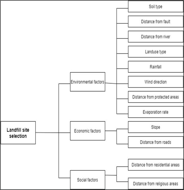
The first part of the course, for this example, is making a hierarchy for decision problems. The goal of the decision problem was landfill site selection for Paveh. The hierarchical construction was built based on the experts’ opinions and earlier studies with convenient data in the study area. In this case, twelve criteria were elected and classified into the principal group. They are demonstrated in Figure 2. Group number one was environmental criteria that involve soil type, distance from the river, distance from fault, land use type, rainfall, distance from protected areas, wind direction and evaporation rate. Group number two was economic criteria including slope and distance from road sub-criteria, and group number three criteria were the social factors, which include distance from residential areas and distance from religious areas [9].

Figure 2.

Hierarchical structure.

4. Formation of pairwise comparison matrices

At this stage, the elements of each level are compared to other related elements at a higher level in a pairwise manner, and pairwise comparison matrices were formed [18]. Allocation of numerical points related to the pairwise comparison of the importance of two options or two indicators is done based on Table 1.

The Intensity of Importance	Description
1	Equal importance
2	Equal to average importance
3	Average importance
4	Average to strong importance
5	Strong importance
6	Strong to very strong importance
7	Very strong importance
8	Very strong or super strong importance
9	Super strong importance
2, 4, 6, 8	Intermediate values

Table 1

Saaty and Vargas preference scales [4].

A pairwise comparison matrix is show below:

$$\left[\begin{array}{cccc}{a}_{11}& a_{12}& \dots & a_{1n}\\ a_{21}& a_{22}& \dots & a_{2n}\\ \dots & \dots & \dots & \dots \\ a_{n1}& a_{n2}& \dots & a_{\mathit{nn}}\end{array}\right]$$E1

where a_ij is the preference of element i over element j. In the pairwise comparison of the criteria with each other, the following relationship is established according to the inverse condition [19];

$$a_{\mathit{ij}}=\frac{1}{a_{\mathit{ji}.}}$$E2

The pairwise comparison matrix is an n × n matrix where n is the number of elements that have been compared [20].

For each pairwise comparison matrix n × n, elements on the diameter are equal to one, and there is no need to evaluate, but other parameters of the matrix must be determined based on pairwise comparisons.

The relative diameters are inverse to each other. Therefore, the number of pairwise comparisons for each n × n pairwise comparison matrix is equal to the [21]:

$$N_c=\frac{n\left(n-1\right)}{2}$$E3

If the decision problem includes m options and n criteria, then n matrices m × m matrices and an n × n comparison matrix should be created. Therefore, the number of pairwise comparisons of the hierarchy (total problem) is equal to the

$$N_h=\frac{\mathrm{n}\left(\mathrm{n}-1\right)}{2}+\left(n\times \frac{m\left(m-1\right)}{2}\right)$$E4

Here, we discuss the pair of criteria comparisons that we designed in the landfill location questionnaire. These questions were asked to two experts in the field of environment and one person in Paveh Municipality and an educated native of that area, and finally, we measured their opinions together and obtained an average and entered the data into the Expert Choice software for review and weighting.

Question: In choosing the right place for the landfill center of Paveh city, is the criterion more important than your point of view? (Table 2)

Choosing landfill place	Environmental factor	Economic factor	Social factor
Environmental factor	1
Economic factor		1
Social factor			1

Table 2.

Determining the weight of the main criteria

Question: If only environmental and health criteria are considered in choosing the right place for the burial center, then which sub-criteria of the table below will be more important? (Table 3)

Environmental factor	Soil type	Distance from fault	Distance from river	Land use type	Rainfall	Wind direction	Distance from protected areas	Evaporation rate
Soil type	1
Distance from fault		1
Distance from river			1
land use type				1
Rainfall					1
Wind direction						1
Distance from protected areas							1
Evaporation rate								1

Table 3.

Determining the weight of sub-criteria related to environmental and health criteria.

Question: If only economic criteria are considered in choosing the right place for the burial center, then which sub-criteria in the following table will be more important? (Table 4)

Economic factor	Slope	Distance from road
Slope	1
Distance from road		1

Table 4.

Determining the weight of the sub-criteria related to the economic criterion.

Question: If only social criteria are considered in choosing the right place for the burial center, then which sub-criteria of the following table will be more important? (Table 5)

Social factor	Distance from residential areas	Distance from religious areas
Distance from residential areas	1
Distance from religious areas		1

Table 5.

Determining the weight of the sub-criteria related to the social criterion.

5. Calculating the weight of elements in the hierarchical analysis method

In the hierarchical analysis method, the elements of each level are compared in pairs to each of the elements of the higher level, and their weights are computed [22]. These weights are called local priority (weight). Then, by combining the local priority, the overall priority of each option is determined. The weight of the criteria reflects their influence in determining the goal [19]. The weight of each option relative to the criteria is the portion of that option in the relevant criteria. Therefore, the overall priority of each option is obtained from the sum of the product of the weight of each criterion by the weight of the option of that criterion [23].

6. Calculation of local priority

After determining the pairwise comparison matrix, the local priority is calculated. There are different methods to calculate the local priority, which we mention here. You can research for more explanation: least squares method, logarithmic least square method, eigenvector method and approximation methods [24].

Approximation methods: This method will have fewer calculations than the previously mentioned methods, but they will also be less accurate. The most important methods of this method are 1—row sum, 2—column sum, 3—arithmetic mean 4—geometric mean [25].

In the first stage of this model, weighting was done based on the AHP method, for this aim, the criteria were weighted using the Delphi method and the opinion of experts from different fields, the criteria were weighted, and using the AHP method and software (Expert Choice11), Expert Choice software was used for the overall priority. Expert Choice software has many capabilities. One of its efficient cases is performing pairwise group comparisons and robust sensitivity analysis [26]. Pairwise group comparisons are used when more than one respondent is involved in decision-making, and sensitivity analysis is performed to check the weight of the options by changing the criteria. This software was developed by Thomas Saaty and Ernest Forman in 1983 by Expert Choice Inc. [6].

Video for how to work with Expert Choice: https://youtu.be/RzoDdms-6jc

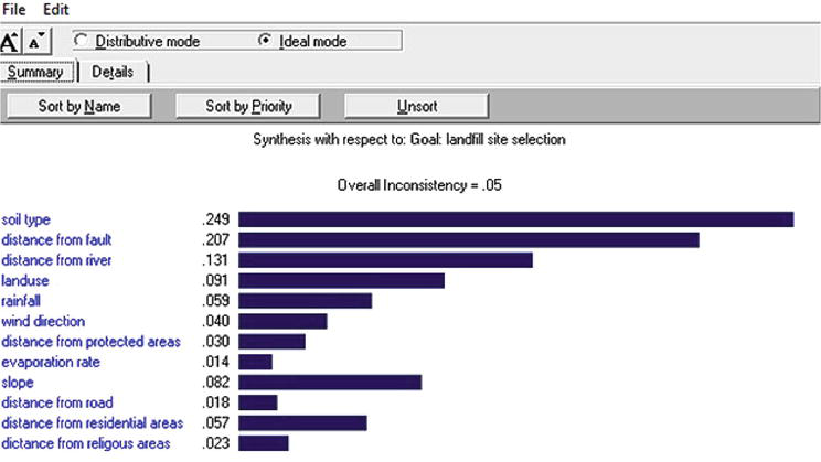
The final weight of the layers was obtained with an inconsistency ratio of 0.05 (which is acceptable based on the Saaty theory, and we will explain this rate in full below). The distance layers from the fault and soil material had the furthest weight (Figure 3).

Figure 3.

Weighting on expert choice.

Inconsistency ratio: One of the advantages of the AHP is to control the consistency of the decision. In other words, A can calculate the compatibility of the decision and judge whether it is good, bad, acceptable or unacceptable. If A is twice as important as B and B is three times as important as C, if the importance of A compared to C is equal to 6, we say this judgment is consistent.

In general, if matrix A has inconsistency, we have the following theorems:

The sum of eigenvalues of matrix A is equal to n:

$$\sum _{\mathrm{i}}{\mathrm{ƛ}}_{\mathrm{i}}=\mathrm{n}$$E5

The eigenvalue of the matrix A is greater than or equal to the dimension of the matrix:

$${ƛ}_{\mathit{max}}\ge n$$E6

When matrix A deviates slightly from the consistent state,${ƛ}_{\mathit{max}}$ will also deviate slightly from n. Therefore, the difference (${ƛ}_{\mathit{max}}$-n) will be an excellent measure to measure the inconsistency of the matrix.

Undoubtedly, the scale (${ƛ}_{\mathit{max}}-n$) depends on the value of n, and to solve this dependence, the scale can be defined as follows, which is called the inconsistency index [12].

$$I.I=\frac{{\mathrm{ƛ}}_{\mathit{max}}-n}{n-1}$$E7

They have calculated the value of the inconsistency index for the matrices whose numbers are entirely randomly chosen and called it the random inconsistency index. The values of (R.I.I) for the n-dimensional matrix can be obtained from the following table [27] (Table 6):

n	1	2	3	4	5	6	7	8	9	10	12
RI	0	0	0.58	0.9	1.12	1.24	1.32	1.45	1.45	1.51	1.53

Table 6

Values of (R.I.I) for the n-dimensional matrix.

For each matrix, the result of dividing the inconsistency index by the random inconsistency index is called the inconsistency rate [28], which is a suitable criterion for judging inconsistency.

For each matrix, the result of dividing the inconsistency index by the random inconsistency index is called the inconsistency rate, which is a suitable criterion for judging inconsistency [29].

$$I.R=\frac{I.I}{R.I.I}$$E8

Calculating the inconsistency rate is also very important in the AHP method. In general, it can be said that the acceptable level of the inconsistency of a system depends on the decision-maker. Still, Saaty presents the number 0.1 as an acceptable limit and believes that if the amount of inconsistency is more than 0.1, it is better to revise the judgment [30].

Here, we will examine an example to understand the calculation of the inconsistency rate better. Then, we will go to the final solution of solving the general example and draw conclusions from it.

For the following pairwise comparison matrix, determine the weight vector from the arithmetic mean method and calculate its inconsistency rate.

	$C_1$	$C_2$	$C_3$
$C_1$	1	2	3
$C_2$	1/3	1	1/4
$C_3$	1/2	4	1

Solve: Arithmetic normalization is as follows: The elements of each column are added together, and each element is divided by this sum.

	$C_1$	$C_2$	$C_3$
$C_1$	0.545	0.375	0.6154
$C_2$	0.181	0.125	0.077
$C_3$	0.272	0.5	0.307

The weight vector comes from the linear average of the elements:

$$C_1·\mathit{0.512}$$E9

$$C_2·\mathit{0.128}$$E10

$$C_3·\mathit{0.360}$$E11

From the multiplication of the weight vector in the matrix, we have a pairwise comparison:

$$\left|\begin{array}{ccc}1& 3& 2\\ 1/3& 1& 1/4\\ 1/2& 4& 1\end{array}\right|\times \left|\begin{array}{c}0.512\\ 0.128\\ 0.360\end{array}\right|=\left|\begin{array}{c}1.616\\ 0.388\\ 1.128\end{array}\right|$$E12

In this case, the values of ƛ and ${ƛ}_{\mathit{max}}$ are calculated as follows:

$${ƛ}_1=\frac{1.616}{0.512}=\mathit{3.156}$$E13

$${ƛ}_2=\frac{0.388}{0.128}=\mathit{3.036}$$E14

$${ƛ}_3=\frac{1.128}{0.360}=\mathit{3.133}$$E15

$${ƛ}_{\mathit{max}}=\frac{3.156+3.0356+3.133}{3}=\mathit{3.108}$$E16

The inconsistency index

$$I.I=\frac{{ƛ}_{\mathit{max}}-n}{n-1}=\frac{3.108-3}{3-1}=\mathit{0.054}$$E17

$$\mathrm{R}.\mathrm{I}.\mathrm{I}\text{from}\mathbf{\text{Table 6}}=\mathit{0.58}$$E18

$$I.R=\frac{I.I}{R.I.I}=\frac{0.054}{0.58}=\mathit{0.093}$$E19

7. Result and discussion

In the initial explanation of this chapter, we will further examine the AHP method based on an example previously worked by the author. The general results for the purpose of determining the location of the landfill for the desired area are shown in the form of a map below (Figures 4–6).

Figure 4.

Final map of landfill suitability.

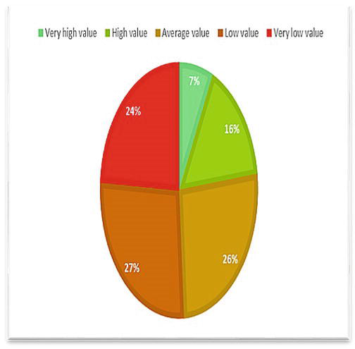
Figure 5.

Exhibition values with percentages.

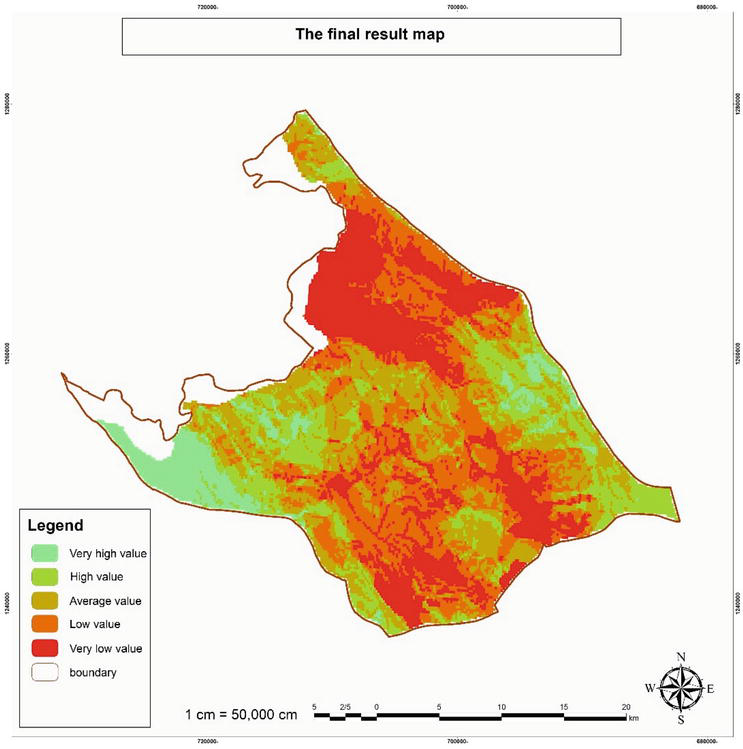
Figure 6.

Final landfill suitability map.

The weight of the layers must first be obtained; for this purpose, using Delphi method and the opinion of expert’s in various fields, the criteria were weighted, and using AHP method and software (Expert Choice11), the final weight of the layers was calculated with an incompatibility coefficient of 0.05, in which the distance layers from the fault and soil material had the highest weight. In this chapter, an attempt was made to refer to the investigation of all ways of weighing and to understand it by giving a simple example.

In Figure 6, the final results of this investigation are shown with the help of GIS software and categorizing all the conditions from high to low value.

The result in Figure 5 shows that 27% has poor landfill (orange), 26% has medium landfill (yellow), 24% of the study area has very poor landfill (red), 16% has good landfill (light green), and 7% has a very high capacity (dark green) for landfilling.

8. Conclusion

In this example, the full explanation of the AHP process, the selection method for weighting and the design of the questionnaire and reaching the right answer using the Expert Choice software and its integration with GIS were discussed. GIS is a powerful software that can provide rapid and perfect evaluation and has a great ability to manage massive volumes of data from different sources; AHP, on the other hand, is a strong way to solve complex problems. Integrating of GIS and AHP methods provides decision-makers with a perfect and immediate review at the lowest cost. In this example, the decision-making process began by examining 12 criteria and obtaining available information based on the criteria for each layer and combined them, then by designing a questionnaire and used the experts opinion to weight the criteria with the AHP method and finally with the help of These weighted layers which are combined in GIS software.

The present study showed that very suitable landfills for the waste of Paveh county cover an area of 51.68794 km² or about 7% of the total classified sites.

Acknowledgments

I would like to thank dear editor Ivana Barac, who patiently followed the work steps on my behalf, and Professor Fabio De Felice, who gave me this opportunity.

References

1.Saaty TL. Decision making with the analytic hierarchy process. International Journal of Services Sciences. 2008;1(1):83-98
2.Bhushan N, Rai K. Strategic Decision Making: Applying the Analytic Hierarchy Process. Springer Science & Business Media; 2007
3.Khaira A, Dwivedi R. A state of the art review of analytical hierarchy process. Materials Today: Proceedings. 2018;5(2):4029-4035
4.Janssen M, van der Voort H, Wahyudi A. Factors influencing big data decision-making quality. Journal of Business Research. 2017;70:338-345
5.Albayrak E, Erensal YC. Using analytic hierarchy process (AHP) to improve human performance: An application of multiple criteria decision making problem. Journal of Intelligent Manufacturing. 2004;15(4):491-503
6.Forman EH, Selly MA. Decision by Objectives: How to Convince Others that you Are Right. World Scientific; 2001
7.Eastman JR, Jiang H, Toledano J. Multi-criteria and multi-objective decision making for land allocation using GIS. In: Multicriteria Analysis for Land-Use Management. Springer; 1998. pp. 227-251
8.Saaty TL, Bennett J. A theory of analytical hierarchies applied to political candidacy. Behavioral Science. 1977;22(4):237-245
9.Rostampoor M, Zamani M, Vaighan A. Combining GIS and analytical hierarchy process for landfill siting, study area: Paveh County in Iran. Journal of Civil Engineering Frontiers. 2020;1(1):07-15
10.Kazakidis V, Mayer Z, Scoble M. Decision making using the analytic hierarchy process in mining engineering. Mining Technology. 2004;113(1):30-42
11.Ramanathan R. A note on the use of the analytic hierarchy process for environmental impact assessment. Journal of Environmental Management. 2001;63(1):27-35
12.Danesh D, Ryan M, Abbasi A. Using analytic hierarchy process as a decision-making tool in project portfolio management. WASET International Journal of Economics and Management Engineering. 2015;9(12):4194-4204
13.Bascetin A. A decision support system using analytical hierarchy process (AHP) for the optimal environmental reclamation of an open-pit mine. Environmental Geology. 2007;52(4):663-672
14.Saaty TL. Decision Making for Leaders: The Analytic Hierarchy Process for Decisions in a Complex World. RWS Publications; 2001
15.Harker PT. The art and science of decision making: The analytic hierarchy process. In: The Analytic Hierarchy Process. Springer; 1989. pp. 3-36
16.Nagesha N, Balachandra P. Barriers to energy efficiency in small industry clusters: Multi-criteria-based prioritization using the analytic hierarchy process. Energy. 2006;31(12):1969-1983
17.Saaty RW. The analytic hierarchy process—What it is and how it is used. Mathematical Modelling. 1987;9(3–5):161-176
18.Saaty TL. What is the analytic hierarchy process? In: Mathematical Models for Decision Support. Springer; 1988. pp. 109-121
19.Sadeghpour M, Mohammadi M. Evaluating traffic risk indexes in Iran’s rural roads. Case study: Ardabil-Meshkin rural road. Transport and Telecommunication. 2018;19(2):103
20.Stein WE, Mizzi PJ. The harmonic consistency index for the analytic hierarchy process. European Journal of Operational Research. 2007;177(1):488-497
21.Lin Z-C, Yang C-B. Evaluation of machine selection by the AHP method. Journal of Materials Processing Technology. 1996;57(3–4):253-258
22.Sinuany-Stern Z, Mehrez A, Hadad Y. An AHP/DEA methodology for ranking decision making units. International Transactions in Operational Research. 2000;7(2):109-124
23.Jankowski P. Integrating geographical information systems and multiple criteria decision-making methods. International Journal of Geographical Information Systems. 1995;9(3):251-273
24.Mikhailov L, Singh MG. Comparison analysis of methods for deriving priorities in the analytic hierarchy process. In: IEEE SMC'99 Conference Proceedings. 1999 IEEE International Conference on Systems, Man, and Cybernetics (Cat. No. 99CH37028). IEEE; 1999
25.Saaty TL, Vargas LG. Comparison of eigenvalue, logarithmic least squares and least squares methods in estimating ratios. Mathematical Modelling. 1984;5(5):309-324
26.Calantone RJ, Di Benedetto CA, Schmidt JB. Using the analytic hierarchy process in new product screening. Journal of Product Innovation Management. 1999;16(1):65-76
27.Saaty TL, Vargas LG. Prediction, Projection and Forecasting: Applications of the Analytic Hierarchy Process in Economics, Finance, Politics, Games and Sports. Springer; 1991
28.Wagner ED. Public Key Infrastructure (PKI) and Virtual Private Network (VPN) Compared Using an Utility Function and the Analytic Hierarchy Process (AHP). Virginia Tech; 2002
29.Marinoni O. Implementation of the analytical hierarchy process with VBA in ArcGIS. Computers & Geosciences. 2004;30(6):637-646
30.Saaty TL, Vargas LG. The decision by the US congress on China’s trade status: A multicriteria analysis. In: Models, Methods, Concepts & Applications of the Analytic Hierarchy Process. Springer; 2001. pp. 305-317
Written By
Mahya Rostampoor
Submitted: 05 December 2022Reviewed: 09 December 2022Published: 10 February 2023
Open access peer-reviewed chapter