Mathematical Modeling of a Three-Phase Induction Motor

Abstract

The induction machine (IM) due to its simplicity of design and maintenance has been favored by manufacturers since its invention by N. Tesla, when he discovered the rotating magnetic fields generated by a system of polyphase currents. However, this simplicity reaches great physical complexity, related to the electromagnetic interactions between the stator and the rotor, which is why it has long been used in constant-speed drives. The induction machine is currently the most widely used electric machine in the industry. Its main advantages lie in the absence of rotor winding, simple structure, robust, and easy to build. A mathematical model is used to represent or reproduce a given real system. The interest of a model is the analysis and prediction of the static and dynamic behavior of the physical system. This chapter’s goals are to provide an overview of a three-phase induction machine’s mathematical model, and its transformation into the two-phase $\left(\alpha ,\beta \right)$ Concordia system.

1. Introduction

Induction machine (IM) is widely used in industrial applications. Indeed, due to its design, its cost is low compared to that of other machines. It is also very robust under different conditions of use. However, the relative simplicity of the machine’s design hides a great functional complexity.

IM depending on whether it is wound rotor or squirrel cage contains a stator and a rotor, made up of silicon steel sheets stack, and containing notches in which the windings are placed, the latter being arranged in such a way that, when supplied by a three-phase electric power produces a rotating field at the frequency of the power supply. This rotating field results in the generation of eddy currents (also called Foucault’s currents) in the rotor bars where a large force results from the interaction of the stator and rotor magnetic fields causing the torque to be generated. However, the squirrel cage structure is often taken during modeling as electrically equivalent to that of a wound rotor whose windings are short-circuited.

The objective of this chapter is to present mathematically the modeling of the induction machine in the form of different state models according to the chosen reference frame. These models are defined in a two-phase frame of reference, either rotating $\left(\mathit{dq}\right)$, or fixed to the stator $\left(\mathit{\alpha \beta }\right)$, the latter is determined from the conventional three-phase reference frame of the induction machine using suitable mathematical transformations.

2. Operating principle

To operate the machine in motor mode, the rotor must be rotated in the direction of the rotating magnetic field, at a speed lower than the synchronous speed (the speed of the rotating field), that is expressed by the following equation [1]:

$${\Omega }_s\mathbf{=}\frac{60f}{p}$$E1

with

${\Omega }_s$: synchronism speed;

$f$: Electric Network Frequency (ENF);

$p$: number of pole pairs.

The speed at which this machine begins to operate (motor mode operation) when it is linked to the electrical network is just a little bit slower than the speed of the stator magnetic field [2]. If the rotational speed of the rotor becomes the same (synchronous) as that of the magnetic field, no induction appears in the rotor; therefore, no interaction happens with the stator (motor stopped) [3]. Finally, if the rotation speed of the rotor is slightly higher than that of the stator magnetic field (generator mode operation), an electromagnetic force similar to that obtained with a synchronous generator will be developed [4]. The difference between the rotation speed of the rotor and that of the magnetic field is called the slip [5], and practically its value does not exceed few percent.

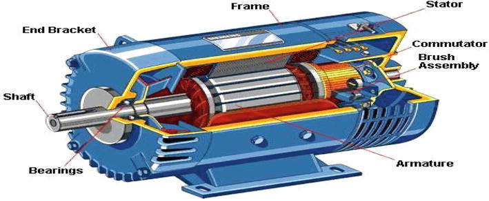
However, from a certain rotational speed, a noticeable decrease in the motor’s stator flux occurs, which requires more current for a similar torque. After reaching a maximum torque value, a reduction in torque and consequently electrical power is observed. Figure 1 illustrates the induction motor components [6].

Figure 1.

Induction motor components [6].

3. Induction machine modeling

3.1 Mathematical model of the induction motor

Modeling of any physical system is necessary in the research filed because it allows researchers to predict how the system can be improved against various phenomena, and thus, learn more about the mechanisms that control it. The induction machine can be modeled by different methods, depending on the desired purposes. The following models are developed in this chapter:

• Models in $\mathit{abc}$ frame, resulting from differential equations controlling the operation of the machine. They are used mainly for the steady-state study [7, 8].

• The models resulting from Concordia’s transformation are commonly used for the dynamic-state study and for the direct torque control (DTC) [9].

3.2 Simplifying assumptions

An induction machine, with its windings distribution and geometry, is so complex that it cannot be analyzed, taking into account its exact configuration. Then, it is necessary to adopt simplifying assumptions [10, 11]:

• The constant air gap;

• The neglected notching effect;

• Sinusoidal spatial distribution of magneto-motor air forces;

• Unsaturated magnetic circuit with constant permeability;

• Negligible ferromagnetic losses;

• The skin effect and warming effect on the characteristics are not taken into account.

Among the important consequences of these assumptions are.

• The association of flux;

• The self-inductances constancy;

• The invariance of stator resistances and rotor resistances;

• The sinusoidal variation law of the mutual inductances between the stator and rotor windings in terms of the electric angle of their magnetic axes;

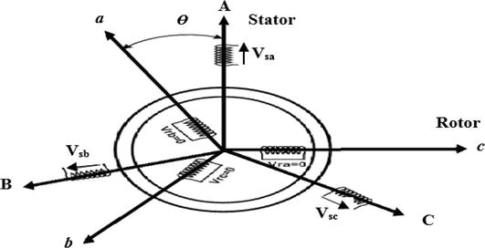
The induction machine is represented schematically by Figure 2. It has six windings:

• The machine stator consists of three fixed windings shifted by 120° in space and crossed by three variable currents.

• The rotor can be modeled by three identical windings shifted in space by 120°. These windings are short circuits and the voltage across them is zero.

Figure 2.

Representation of the induction machine.

3.3 Induction machine modeling

Aforesaid, to ensure motor operation, the IM’s rotation speed must be lower than the synchronization speed (positive slip). Unlike the synchronous machine, the IM does not have a separate inductor; therefore, it requires a reactive power input for its magnetization. When it connected directly to the grid, the latter provides the required reactive power. On the other hand, in autonomous operation, it is necessary to bring this energy either by a battery of capacitors or by a controlled static converter (an inverter).

A mathematical model is necessary for the analysis of the IM’s operation in both motor and generator modes. The analytical modeling will be presented in the section below.

3.3.1 Electrical equations of the induction machine in the three-phase reference

The induction machine is of three-phase nature. Taking into account the assumptions mentioned above and using the diagram shown in Figure 3, the induction machine’s basic equations are [12, 13]:

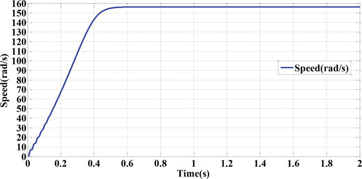
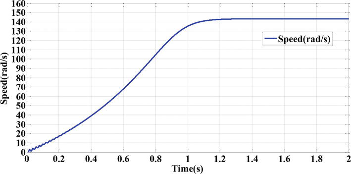
Figure 3.

Rotor speed simulation result.

$${\left[v_{\mathit{\text{sabc}}}\right]}^T=\left[R_s\right]{\left[i_{\mathit{\text{sabc}}}\right]}^T+\frac{d}{\mathit{dt}}{\left[{\phi }_{\mathit{\text{sabc}}}\right]}^T$$E2

$${\left[v_{\mathit{\text{rabc}}}\right]}^T=0=\left[R_r\right]{\left[i_{\mathit{\text{rabc}}}\right]}^T+\frac{d}{\mathit{dt}}{\left[{\phi }_{\mathit{\text{rabc}}}\right]}^T$$E3

With.

$v_{\mathit{\text{sabc}}}$: The voltages applied to the three-stator phases.

$i_{\mathit{\text{sabc}}}$: The currents that cross the three-stator phases.

${\phi }_{\mathit{\text{sabc}}}$: The total flux through these windings.

$R_s$: The stator resistance.

$R_r$: The rotor resistance.

Each flux comprises an interaction with the currents of all the phases including its own.

$$\left[\begin{array}{c}\begin{array}{c}{\phi }_{\mathit{sa}}\\ {\phi }_{\mathit{sb}}\\ {\phi }_{\mathit{sc}}\end{array}\\ \begin{array}{c}{\phi }_{\mathit{ra}}\\ {\phi }_{\mathit{rb}}\\ {\phi }_{\mathit{rc}}\end{array}\end{array}\right]=\left[\begin{array}{cc}\begin{array}{ccc}{l}_s& m_s& m_s\\ m_s& l_s& m_s\\ m\_\mathrm{s}& m_s& l_s\end{array}& \begin{array}{ccc}{m}_1& m_3& m_2\\ m_2& m_1& m_3\\ m_3& m_2& m_1\end{array}\\ \begin{array}{ccc}{m}_1& m_2& m_3\\ m_3& m_1& m_2\\ m_2& m_3& m_1\end{array}& \begin{array}{ccc}{l}_r& m_r& m_r\\ m_r& l_r& m_r\\ m_r& m_r& l_r\end{array}\end{array}\right]\left[\begin{array}{c}\begin{array}{c}{i}_{\mathit{sa}}\\ i_{\mathit{sb}}\\ i_{\mathit{sc}}\end{array}\\ \begin{array}{c}{i}_{\mathit{ra}}\\ i_{\mathit{rb}}\\ i_{\mathit{rc}}\end{array}\end{array}\right]$$E4

where.

$l_s$ is the self-inductance of a stator phase.

$l_r$ is the self-inductance of a rotor phase.

$m_s$ is the mutual inductance between two stator phases.

$m_r$ is the mutual inductance between two rotor phases.

$m_{\mathit{sr}}$ is the maximum mutual inductance between a stator phase and a rotor phase.

$$m_1=m_{\mathit{sr}}cos\left(\theta \right)$$E5

$$m_2=m_{\mathit{sr}}cos\left(\theta -\frac{2\pi }{3}\right)$$E6

$$m_3=m_{\mathit{sr}}cos\left(\theta +\frac{2\pi }{3}\right)$$E7

3.3.2 Three-phase/two-phase transformation (Concordia and Clarke transformation)

The aim of using this transformation is to switch from a three-phase $\mathit{abc}$ system to the stationary two-phase $\mathit{\alpha \beta }$ system [14, 15, 16]. There are mainly two transformations: Clarke and Concordia transformations. The magnitude of the converted quantities is saved by Clarke transformation, but neither the power nor the torque is (we must multiply by a coefficient of 3/2) [17]. While Concordia transformations keeps the power but not the magnitude (Tables 1 and 2) [18].

Concordia transformation

Clarke transformation

$\left[\begin{array}{c}{\mathit{x}}_{\mathit{a}}\\ {\mathit{x}}_{\mathit{b}}\\ {\mathit{x}}_{\mathit{c}}\end{array}\right]\stackrel{{\mathit{T}}_{\mathbf{23}}}{\to }\left[\begin{array}{c}{\mathit{x}}_{\mathit{\alpha }}\\ {\mathit{x}}_{\mathit{\beta }}\end{array}\right]$ i.e. ${\left[{\mathit{x}}_{\mathit{\alpha \beta }}\right]}^{\mathit{T}}\mathit{=}{\mathit{T}}_{\mathbf{23}}{\left[{\mathit{x}}_{\mathit{abc}}\right]}^{\mathit{T}}$; with: ${\mathit{T}}_{\mathbf{23}}\mathit{=}\sqrt{\frac{\mathbf{2}}{\mathbf{3}}}\left[\begin{array}{ccc}\mathbf{1}& \mathit{-}\frac{\mathbf{1}}{\mathbf{2}}& \mathit{-}\frac{\mathbf{1}}{\mathbf{2}}\\ \mathbf{0}& \frac{\sqrt{\mathbf{3}}}{\mathbf{2}}& \mathit{-}\frac{\sqrt{\mathbf{3}}}{\mathbf{2}}\end{array}\right]$

$\left[\begin{array}{c}{x}_a\\ x_b\\ x_c\end{array}\right]\stackrel{C_{23}}{\to }\left[\begin{array}{c}{x}_{\alpha }\\ x_{\beta }\end{array}\right]$i.e. ${\left[x_{\mathit{\alpha \beta }}\right]}^T=C_{23}{\left[x_{\mathit{abc}}\right]}^T$; with: $C_{23}=\frac{2}{3}\left[\begin{array}{ccc}1& -\frac{1}{2}& -\frac{1}{2}\\ 0& \frac{\sqrt{3}}{2}& -\frac{\sqrt{3}}{2}\end{array}\right]$

Table 1.

Concordia and Clarke transformations.

Inverse Concordia transformation

Inverse Clarke transformation

$\left[\begin{array}{c}{x}_{\alpha }\\ x_{\beta }\end{array}\right]\stackrel{T_{32}}{\to }\left[\begin{array}{c}{x}_a\\ x_b\\ x_c\end{array}\right]$ i.e. ${\left[x_{\mathit{abc}}\right]}^T=T_{32}{\left[x_{\mathit{\alpha \beta }}\right]}^T$; with: $T_{32}=\sqrt{\frac{2}{3}}\left[\begin{array}{c}1\\ -\frac{1}{2}\\ -\frac{1}{2}\end{array}\begin{array}{c}0\\ \frac{\sqrt{3}}{2}\\ -\frac{\sqrt{3}}{2}\end{array}\right]$

$\left[\begin{array}{c}{x}_{\alpha }\\ x_{\beta }\end{array}\right]\stackrel{C_{32}}{\to }\left[\begin{array}{c}{x}_a\\ x_b\\ x_c\end{array}\right]$ i.e. ${\left[x_{\mathit{\alpha \beta }}\right]}^T=C_{32}{\left[x_{\mathit{abc}}\right]}^T$; with: $C_{32}=\left[\begin{array}{c}1\\ -\frac{1}{2}\\ -\frac{1}{2}\end{array}\begin{array}{c}0\\ \frac{\sqrt{3}}{2}\\ -\frac{\sqrt{3}}{2}\end{array}\right]$

Table 2.

Transformation of a two-phase $\mathit{\alpha \beta }$ system to a three-phase $\mathit{abc}$ (system).

3.3.3 Three-phase/two-phase transformation (park transformation)

Park transformation is a transformation of the fixed three-phase reference frame relative to the stator in a two-phase reference frame [19]. It allows to move from the $\mathit{abc}$ reference to the ($d,q$) reference, where d refers to the direct axis and q to the quadrature axis. The $\left(\mathrm{\alpha },\mathrm{\beta }\right)$reference frame is always fixed according to the $\mathrm{abc}$frame [20], where the $\left(d,q\right)$reference frame is mobile [21].

This transformation reduces the complexity of the system. The reference frame position can be fixed according to the three referential [22, 23]:

• Reference system linked to the rotating field.

• Referential linked to the stator.

• Reference system linked to the rotor.

The transformation matrix of Park and its inverse are given by

$$\left\{\begin{array}{c}P\left(\theta \right)=k\left(\begin{array}{ccc}cos\left(\theta \right)& cos\left(\theta -\frac{2\pi }{3}\right)& cos\left(\theta +\frac{2\pi }{3}\right)\\ -sin\left(\theta \right)& -sin\left(\theta -\frac{2\pi }{3}\right)& -sin\left(\theta +\frac{2\pi }{3}\right)\\ \frac{1}{\sqrt{2}}& \frac{1}{\sqrt{2}}& \frac{1}{\sqrt{2}}\end{array}\right)\\ P{\left(\theta \right)}^{-1}=P{\left(\theta \right)}^T=k\left(\begin{array}{ccc}cos\left(\theta \right)& -sin\left(\theta \right)& \frac{1}{\sqrt{2}}\\ cos\left(\theta -\frac{2\pi }{3}\right)& -sin\left(\theta -\frac{2\pi }{3}\right)& \frac{1}{\sqrt{2}}\\ cos\left(\theta +\frac{2\pi }{3}\right)& -sin\left(\theta +\frac{2\pi }{3}\right)& \frac{1}{\sqrt{2}}\end{array}\right)\end{array}\right.$$E8

where $k$ is a constant that can take the value $2/3$ for the transformation with no power conservation or $\sqrt{2/3}$ for the transformation with power conservation [24].

3.4 Model of the induction machine in the park referential

The Park transformation consists in applying to the currents, voltages, and flux a change of variables involving the angle between the windings axis and the axis of the Park $\left(d,q\right)$frame [25].

Eqs. (2), (3), and (4) give rise to the following system [26]:

$$\left\{\begin{array}{c}{v}_{\mathit{sd}}=R_s{i}_{\mathit{sd}}+\frac{d{\varphi }_{\mathit{sd}}}{\mathit{dt}}-{\omega }_s{\phi }_{\mathit{sq}}\\ v_{\mathit{sq}}=R_s{i}_{\mathit{sq}}+\frac{d{\varphi }_{\mathit{sq}}}{\mathit{dt}}+{\omega }_s{\phi }_{\mathit{sd}}\end{array}\right.$$E9

$$\left\{\begin{array}{c}{v}_{\mathit{rd}}=0=R_r{i}_{\mathit{rd}}+\frac{d{\varphi }_{\mathit{rd}}}{\mathit{dt}}-{\omega }_r{\phi }_{\mathit{rq}}\\ v_{\mathit{rq}}=0=R_r{i}_{\mathit{rq}}+\frac{d{\varphi }_{\mathit{rq}}}{\mathit{dt}}+{\omega }_r{\phi }_{\mathit{rd}}\end{array}\right.$$E10

with

$$\left[\begin{array}{c}{\phi }_{\mathit{sdq}}\\ {\phi }_{\mathit{rdq}}\end{array}\right]=\left[\begin{array}{c}{L}_s\\ 0\\ L_m\\ 0\end{array}\begin{array}{c}0\\ L_s\\ 0\\ L_m\end{array}\begin{array}{c}{L}_m\\ 0\\ L_r\\ 0\end{array}\begin{array}{c}0\\ L_m\\ 0\\ L_r\end{array}\right]\left[\begin{array}{c}{i}_{\mathit{sdq}}\\ i_{\mathit{rdq}}\end{array}\right]$$E11

Indeed, the submatrices are now diagonal and no longer depend on $\mathrm{\theta }$(the electrical angle between the stator and the rotor).

The matrix system can also be written as [27]:

$$\left\{\begin{array}{c}{\phi }_{\mathit{sd}}=L_s{i}_{\mathit{sd}}+L_m{i}_{\mathit{rd}}\\ {\phi }_{\mathit{sq}}=L_s{i}_{\mathit{sq}}+L_m{i}_{\mathit{rq}}\end{array}\right.$$E12

$$\left\{\begin{array}{c}{\phi }_{\mathit{rd}}=L_m{i}_{\mathit{sd}}+L_r{i}_{\mathit{rd}}\\ {\phi }_{\mathit{rq}}=L_m{i}_{\mathit{sq}}+L_r{i}_{\mathit{rq}}\end{array}\right.$$E13

(where)

$$L_s=l_s-m_s,L_r=l_r-m_r,L_m=\frac{2}{3}{m}_{\mathit{sr}}$$

We have expressed the machine’s equations, but there also remains the electromagnetic torque. The latter can be derived from the co-energy expression, or obtained using power balance.

The instantaneous power supplied to the stator and rotor windings is written as [28]

$$P_e={\left[V_s\right]}^T\left[I_s\right]+{\left[V_r\right]}^T\left[I_r\right]$$E14

By applying Park transformation, it is expressed in terms of the axes quantity $\mathit{dq}$

$$P_e=\left[v_{\mathit{sd}}{v}_{\mathit{sq}}\right]\left[\begin{array}{c}{i}_{\mathit{sd}}\\ i_{\mathit{sq}}\end{array}\right]+\left[\begin{array}{cc}{v}_{\mathit{rd}}& v_{\mathit{rq}}\end{array}\right]\left[\begin{array}{c}{i}_{\mathit{rd}}\\ i_{\mathit{rq}}\end{array}\right]=\underset{\mathit{\text{first term}}}{\underbrace{\frac{2}{3}\left[i_{\mathit{sd}}\frac{d{\phi }_{\mathit{sd}}}{\mathit{dt}}+i_{\mathit{sq}}\frac{d{\phi }_{\mathit{sq}}}{\mathit{dt}}+i_{\mathit{rd}}\frac{d{\phi }_{\mathit{rd}}}{\mathit{dt}}+i_{\mathit{rq}}\frac{d{\phi }_{\mathit{rq}}}{\mathit{dt}}\right]}}$$

$$+\underset{\mathit{\text{second term}}}{\underbrace{\frac{2}{3}\left[\left({\phi }_{\mathit{sd}}{i}_{\mathit{sq}}-{\phi }_{\mathit{sq}}{i}_{\mathit{sd}}\right){\omega }_s+\left({\phi }_{\mathit{rq}}{i}_{\mathit{rd}}-{\phi }_{\mathit{rd}}{i}_{\mathit{rq}}\right){\omega }_r\right]}}$$E15

$$+\underset{\mathit{\text{third term}}}{\underbrace{\frac{2}{3}\left[R_s\left(i_{\mathit{sd}}^2+i_{\mathit{sq}}^2\right)+R_r\left(i_{\mathit{rd}}^2+i_{\mathit{rq}}^2\right)\right]}}$$

• The first term represents the magnetic energy stored in iron.

• The second term represents the electromechanical power $P_{\mathit{em}}$of the machine.

• The third term represents joule losses.

Taking into account the flux Eqs. (12) and (13), several equal expressions result

$$\left\{\begin{array}{l}{\Gamma }_{\mathit{em}}=p\left({\phi }_{\mathit{sd}}{i}_{\mathit{sq}}–{\phi }_{\mathit{sq}}{i}_{\mathit{sd}}\right)\\ {\Gamma }_{\mathit{em}}=p\left({\phi }_{\mathit{rq}}{i}_{\mathit{rd}}-{\phi }_{\mathit{rd}}{i}_{\mathit{rq}}\right)\\ {\Gamma }_{\mathit{em}}=p{L}_m\left(i_{\mathit{sq}}{i}_{\mathit{rd}}-i_{\mathit{sd}}{i}_{\mathit{rq}}\right)\\ {\Gamma }_{\mathit{em}}=p\frac{L_m}{L_r}\left({\phi }_{\mathit{rd}}{i}_{\mathit{sq}}-{\phi }_{\mathit{rq}}{i}_{\mathit{sd}}\right)\end{array}\right.$$E16

where $p$ is the number of poles pairs. The power $P_{\mathit{em}}$is also equal to ${\Gamma }_{\mathit{em}}{\omega }_r/p$, and the movement equation is [29]

$${\Gamma }_{\mathit{em}}-{\Gamma }_r=f{\mathrm{\Omega }}_m+J\frac{d{\mathrm{\Omega }}_m}{\mathit{dt}}$$E17

3.5 Selecting the $\mathit{dq}$ (frame)

The machine’s equations and electrical quantities have been expressed thus far in a reference $\mathit{dq}$, which makes an electrical angle ${\mathrm{\theta }}_s$ and ${\mathrm{\theta }}_r$ with the stator and with the rotor respectively, but which is not defined elsewhere, that is, it is free [30, 31].

According to the application purpose, there are three main choices for the axis $\left(d,q\right)$ frame orientation: a frame linked to the stator, rotor, or linked to the rotating field [32, 33]. In each of these referential, the equations of the machine become simpler than in any other referential [34]. Generally, the operating conditions will typically determine the most convenient reference for analysis and/or simulation purposes.

3.5.1 Reference linked to the stator

Regarding the stator, this referential is immobile. It is carried out to investigate machine braking and starting (i.e., this reference frame is better adapted to work with instantaneous quantities) [35]. In addition, this choice is used for direct torque control design [36].

It is characterized by.

$\mathrm{\omega }={\mathrm{\omega }}_s=0$ and therefore, ${\mathrm{\omega }}_r=-{\mathrm{\omega }}_m$ (where $\mathrm{\omega }$ is the arbitrary frame rate).

The system of equations in this reference frame is [37, 38, 39]

$$\left\{\begin{array}{l}{v}_{\mathit{sd}}=R_s{i}_{\mathit{sd}}+\frac{d{\phi }_{\mathit{sd}}}{\mathit{dt}}\\ v_{\mathit{sq}}=R_s{i}_{\mathit{sq}}+\frac{d{\phi }_{\mathit{sq}}}{\mathit{dt}}\\ v_{\mathit{rd}}=0=R_r{i}_{\mathit{rd}}+\frac{d{\phi }_{\mathit{rd}}}{\mathit{dt}}-{\omega }_r{\phi }_{\mathit{rq}}\\ v_{\mathit{rq}}=0=R_r{i}_{\mathit{rq}}+\frac{d{\phi }_{\mathit{rq}}}{\mathit{dt}}+{\omega }_r{\phi }_{\mathit{rd}}\end{array}\right.$$E18

3.5.2 Reference linked to the rotor

In the case where the $\left(d,q\right)$ reference frame is synchronized with the rotor $\mathrm{\omega }={\mathrm{\omega }}_s={\mathrm{\omega }}_m$ and ${\mathrm{\omega }}_r=0$. This reference frame is used for the simulation of the dynamic state of machines where the speed is assumed constant [40]. In this case, the system of equations is [41]

$$\left\{\begin{array}{l}{v}_{\mathit{sd}}=R_s{i}_{\mathit{sd}}+\frac{d{\phi }_{\mathit{sd}}}{\mathit{dt}}-{\omega }_s{\phi }_{\mathit{sq}}\\ v_{\mathit{sq}}=R_s{i}_{\mathit{sq}}+\frac{d{\phi }_{\mathit{sq}}}{\mathit{dt}}+{\omega }_s{\phi }_{\mathit{sd}}\\ v_{\mathit{rd}}=0=R_r{i}_{\mathit{rd}}+\frac{d{\phi }_{\mathit{rd}}}{\mathit{dt}}\\ v_{\mathit{rq}}=0=R_r{i}_{\mathit{rq}}+\frac{d{\phi }_{\mathit{rq}}}{\mathit{dt}}\end{array}\right.$$E19

3.5.3 Reference linked to the rotating magnetic field

This choice allows obtaining a sliding pulsation and properly adapts vector control through rotor flux orientation [42]. The reference frame linked to the synchronism (or rotating field) is fixed relative to the rotating field. It is used for the machine vector control and it is characterized by $\mathrm{\omega }={\mathrm{\omega }}_s$, which implies that the adjustment variables are continuous [43]. The advantage of using this reference frame is to have constant quantities in steady state; then, it is easier to carry out the regulation [44]. Then, we can write [45]

$$\left\{\begin{array}{l}{v}_{\mathit{sd}}=R_s{i}_{\mathit{sd}}+\frac{d{\phi }_{\mathit{sd}}}{\mathit{dt}}-{\omega }_s{\phi }_{\mathit{sq}}\\ v_{\mathit{sq}}=R_s{i}_{\mathit{sq}}+\frac{d{\phi }_{\mathit{sq}}}{\mathit{dt}}+{\omega }_s{\phi }_{\mathit{sd}}\\ v_{\mathit{rd}}=0=R_r{i}_{\mathit{rd}}+\frac{d{\phi }_{\mathit{rd}}}{\mathit{dt}}-{\omega }_r{\phi }_{\mathit{rq}}\\ v_{\mathit{rq}}=0=R_r{i}_{\mathit{rq}}+\frac{d{\phi }_{\mathit{rq}}}{\mathit{dt}}+{\omega }_r{\phi }_{\mathit{rd}}\end{array}\right.$$E20

These equations can be rewritten to have a different state vector (state variables system), that is, instead of having the flux, we can write it in currents; we just need to make substitutions of Eqs. (12) and (13) in Eq. (20).

3.6 Model of the induction machine in the $\left(\alpha ,\beta \right)$ (frame)

The dynamic model of an induction motor can be developed from its basic electrical and mechanical equations [46]. In the stationary reference frame, the voltages are expressed as follows [47]:

$$\left\{\begin{array}{l}{v}_{\mathit{s\alpha }}=R_s{i}_{\mathit{s\alpha }}+s{\phi }_{\mathit{s\alpha }}\\ v_{\mathit{s\beta }}=R_s{i}_{\mathit{s\beta }}+s{\phi }_{\mathit{s\beta }}\\ v_{\mathit{r\alpha }}=0=R_r{i}_{\mathit{r\alpha }}+s{\phi }_{\mathit{r\alpha }}+{\omega }_r{\phi }_{\mathit{r\beta }}\\ v_{\mathit{r\beta }}=0=R_r{i}_{\mathit{r\beta }}+s{\phi }_{\mathit{r\beta }}-{\omega }_r{\phi }_{\mathit{r\alpha }}\end{array}\right.$$E21

where $s$ indicates the differential operator $\left(d/\mathit{dt}\right).$

The stator and rotor fluxes equations are [48]

$$\left\{\begin{array}{l}{\phi }_{\mathit{s\alpha }}=L_s{i}_{\mathit{s\alpha }}+L_m{i}_{\mathit{r\alpha }}\\ {\phi }_{\mathit{s\beta }}=L_s{i}_{\mathit{s\beta }}+L_m{i}_{\mathit{r\beta }}\\ {\phi }_{\mathit{r\alpha }}=L_r{i}_{\mathit{r\alpha }}+L_m{i}_{\mathit{s\alpha }}\\ {\phi }_{\mathit{r\beta }}=L_r{i}_{\mathit{r\beta }}+L_m{i}_{\mathit{s\beta }}\end{array}\right.$$E22

In these equations, $R_s$, $R_r$, $L_s$, and $L_r$ are, respectively, the resistors and the inductances of the stator windings and the rotor windings, $L_m$ is the mutual inductance and ${\mathrm{\omega }}_r=p.{\mathrm{\Omega }}_r$ is the rotor speed (with $p$ is the pairs poles number). Additionally, ${\mathrm{\omega }}_s$ is the synchronous pulsation.

$v_{\mathrm{s\alpha }}$, $v_{\mathrm{s\beta }}$, $v_{\mathrm{r\alpha }}$, $v_{\mathrm{r\beta }}$, $i_{\mathrm{s\alpha }}$, $i_{\mathrm{s\beta }}$, $i_{\mathrm{r\alpha }}$, $i_{\mathrm{r\beta }}$, ${\mathrm{ø}}_{\mathrm{s\alpha }}$, ${\mathrm{ø}}_{\mathrm{s\beta }}$, ${\mathrm{ø}}_{\mathrm{r\alpha }},$ and ${\mathrm{ø}}_{\mathrm{r\beta }}$ are the direct and quadratic components, respectively, of the voltages and currents as well as the fluxes of both the stator and the rotor.

The mechanical equation is [29]

$${\Gamma }_{\mathit{em}}-{\Gamma }_r=f{\mathrm{\Omega }}_m+J\frac{d{\mathrm{\Omega }}_m}{\mathit{dt}}$$E23

where ${\mathrm{\Gamma }}_{\mathit{em}}$ is the electromagnetic torque [N.m] and ${\mathrm{\Gamma }}_r$ is the resistive torque imposed by the machine shaft [N. m].

The electromagnetic torque is [49]

$${\Gamma }_{\mathit{em}}=\frac{3}{2}p\left({\phi }_{\mathit{s\alpha }}{i}_{\mathit{s\beta }}-{\phi }_{\mathit{s\beta }}{i}_{\mathit{s\alpha }}\right)$$E24

For the complete model of the induction machine, the flux expressions are replaced in the voltage equations. We obtain a mechanical equation and four electrical equations in terms of the stator currents, rotor fluxes components, and the electric speed of induction machine as well [45]:

$$\left\{\begin{array}{l}\frac{d{i}_{\mathit{s\alpha }}}{\mathit{dt}}=-\frac{1}{\sigma L_s}\left(R_s+\frac{1}{T_r}\frac{L_m^2}{L_r}\right)i_{\mathit{s\alpha }}+\frac{1}{\sigma L_s}\left(\frac{L_m}{L_r}\frac{1}{T_r}\right){\phi }_{\mathit{r\alpha }}+\frac{1}{\sigma L_s}\left(\frac{L_m}{L_r}\right){\omega }_r{\phi }_{\mathit{r\beta }}\\ \frac{d{i}_{\mathit{s\beta }}}{\mathit{dt}}=-\frac{1}{\sigma L_s}\left(R_s+\frac{1}{T_r}\frac{L_m^2}{L_r}\right)i_{\mathit{s\beta }}-\frac{1}{\sigma L_s}\left(\frac{L_m}{L_r}\right){\omega }_r{\phi }_{\mathit{r\alpha }}+\frac{1}{\sigma L_s}\left(\frac{L_m}{L_r}\frac{1}{T_r}\right){\phi }_{\mathit{r\beta }}\\ \frac{d{\phi }_{\mathit{r\alpha }}}{\mathit{dt}}=\frac{L_m}{T_r}{i}_{\mathit{s\alpha }}-\frac{1}{T_r}{\phi }_{\mathit{r\alpha }}-{\omega }_r{\phi }_{\mathit{r\beta }}\\ \frac{d{\phi }_{\mathit{r\beta }}}{\mathit{dt}}=\frac{L_m}{T_r}{i}_{\mathit{s\alpha }}+{\omega }_r{\phi }_{\mathit{r\alpha }}-\frac{1}{T_r}{\phi }_{\mathit{r\beta }}\end{array}\right.$$E25

Such as ${\omega }_m=p{\mathrm{\Omega }}_m;{\omega }_r=\left[{\omega }_s-{\omega }_m\right];\sigma =1-\frac{L_m^2}{L_s{L}_r};T_r=\frac{L_r}{R_r};T_s=\frac{L_s}{R_s}$.

Modeling the machine in this way that reduces the number of quantities that we need to know in order to simulate machine operation. In fact, only the instantaneous values of the stator voltages and the resistive torque must be determined in order to impose them on the machine. Therefore, we do not need to know the stator pulsation value, or the slip as in the case of the model whose equations are written in the reference frame rotating in synchronism [50].

3.7 Voltage powered machine state space representation

The state space representation of the induction machine depends on the selected frame and the selection of state variables for the electrical equations. We write the equations in the $\left(\mathrm{\alpha },\mathrm{\beta }\right)$ frame because it is the most general and complete solution [51]. The objectives for either the control or the observation determine the state variables to be used [52].

For a three-phase IM powered by voltage, the stator voltages ($v_{\mathrm{s\alpha }},v_{\mathrm{s\beta }}$) are considered as control variables, the load torque ${\mathrm{\Gamma }}_r$ as a disturbance [53]. In our case, we choose the state vector $x={\left[\begin{array}{cc}{i}_{\mathit{s\alpha }}& i_{\mathit{s\beta }}\end{array}\begin{array}{cc}{\phi }_{\mathit{r\alpha }}& {\phi }_{\mathit{r\beta }}\end{array}\right]}^T$, we obtain [39]

$$\dot{x}\left(t\right)=A\left(t\right)x\left(t\right)+B\left(t\right)u\left(t\right)$$E26

with:

$$A\left(t\right)=\left[\begin{array}{c}-\frac{1}{\sigma L_s}\left(R_s+\frac{1}{T_r}\frac{L_m^2}{L_r}\right)\\ 0\\ \frac{L_m}{T_r}\\ 0\end{array}\begin{array}{c}0\\ -\frac{1}{\sigma L_s}\left(R_s+\frac{1}{T_r}\frac{L_m^2}{L_r}\right)\\ 0\\ \frac{L_m}{T_r}\end{array}\begin{array}{c}\frac{1}{\sigma L_s}\left(\frac{L_m}{L_r}\frac{1}{T_r}\right)\\ -\frac{1}{\sigma L_s}\left(\frac{L_m}{L_r}\right){\omega }_r\\ -\frac{1}{T_r}\\ {\omega }_r\end{array}\begin{array}{c}\frac{1}{\sigma L_s}\left(\frac{L_m}{L_r}\right){\omega }_r\\ \frac{1}{\sigma L_s}\left(\frac{L_m}{L_r}\frac{1}{T_r}\right)\\ -{\omega }_r\\ -\frac{1}{T_r}\end{array}\right]$$E27

$$B\left(t\right)=\left[\begin{array}{c}\frac{1}{L_s\sigma }\\ 0\\ 0\\ 0\end{array}\begin{array}{c}0\\ \frac{1}{L_s\sigma }\\ 0\\ 0\end{array}\right]$$E28

$$\text{and}:u\left(t\right)=\left[\begin{array}{c}{v}_{\mathit{s\alpha }}\\ v_{\mathit{s\beta }}\end{array}\right]$$E29

3.8 Simulation results

The purpose of this test is to validate our motor block before using it with space vector PWM (SVPWM) and with direct torque control. Our goal is to integrate it later in the simulations. To carry out the simulation, we translate the mathematical model of the machine using the SimPowerSystem blocks of the Matlab/Simulink software.

3.8.1 No-load test

For an induction machine supplied directly by the 220/380 V three-phase network and running off-load, we visualize the mechanical speed, the electromagnetic torque, the stator currents as well as the components of both the current and the stator fluxes.

The simulation results are represented in the Figures 3–7.

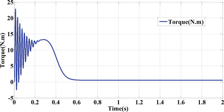
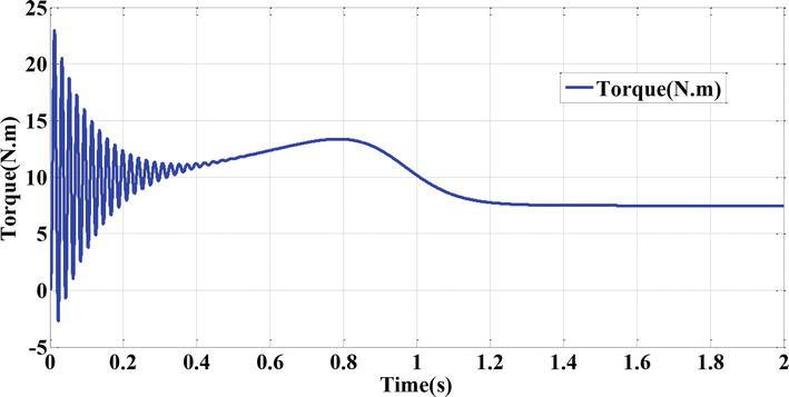
Figure 4.

Magnetic torque simulation result.

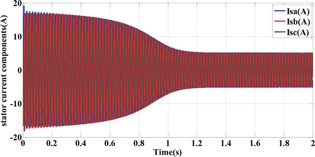
Figure 5.

Stator currents simulation result.

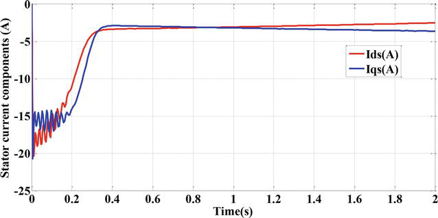
Figure 6.

Stator currents components simulation result.

Figure 7.

Stator flux components simulation result.

The steady-state speed stabilizes at a value close to the synchronism speed because the machine is not loaded. At no-load starting, the torque is strongly pulsating; it reaches a maximum value in the range of 3.2 times the nominal torque. This is due to the noises generated by the mechanical part, and after the disappearance of the transitory mode, it tends toward the value corresponding to the zero load. The absorbed current is high at start-up; it is about three times the rated. At steady state, there remains the current corresponding to the inductive behavior of the no-loaded motor. The rotor current is significant during start-up and drops completely at steady state.

3.8.2 Load variations after no-load starting

Figures 8–12 represent the three-phase currents, the rotational speed, and the electromagnetic torque of the motor, respectively. Two cases are carried out in this simulation with no load and with a loaded motor:

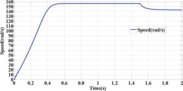
Figure 8.

Rotor speed simulation result.

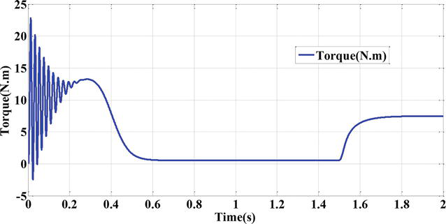
Figure 9.

Magnetic torque simulation result.

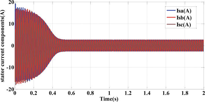
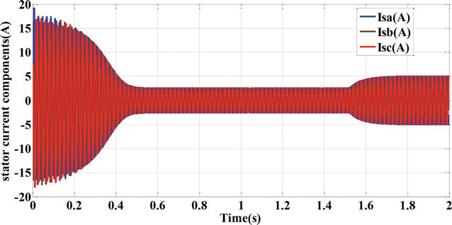
Figure 10.

Stator currents simulation result.

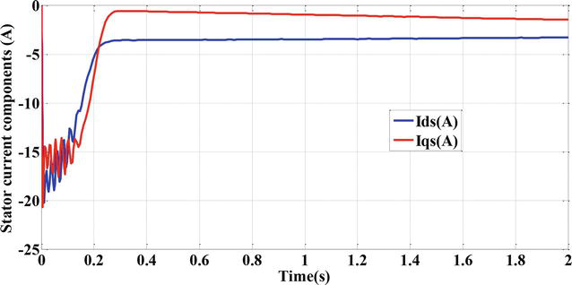
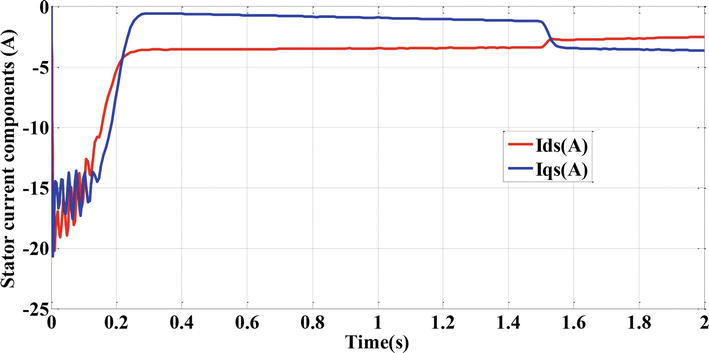
Figure 11.

Stator currents component simulation result.

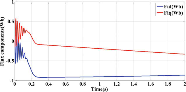
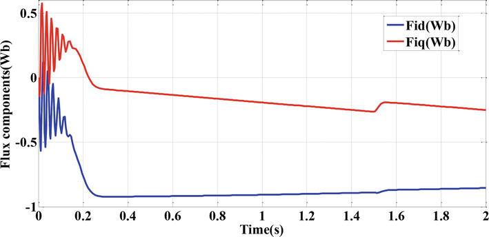
Figure 12.

Stator flux component simulation result.

When the motor run under no load condition, in the dynamic state, we observe an excessively absorbed current that stabilizes to produce a sinusoidal form with constant amplitude.

When the motor is not loaded, we observe at the beginning of the start-up running that the increase in speed is virtually linear, and the total inertia around the rotating shaft determines the speed-up time (about $0.5s$), where the obtained speed is close to $157\mathit{rad}/s.$

Under load: A load torque (${\Gamma }_r=7N.m$) is applied to the machine shaft (at time $t=1.5s$). When the electromagnetic torque reaches the load torque, obviously, there is a reduction in the rotating speed. Additionally, we notice an increase in the stator currents’ magnitude and a slight decrease in the flux.

3.8.3 Starting under load

While starting under load (Figures 13–17), the electromagnetic torque responds instantly (because ${\Gamma }_{\mathit{em}}$ is greater than ${\Gamma }_r$) and the asynchronous motor accelerates, where the speed is slightly disturbed. Without control, a high overshoot response for electromagnetic torque is obtained. Therefore, it is not recommended to be used in an open-loop system for stability reasons.

Figure 13.

Rotor speed simulation result.

Figure 14.

Magnetic torque simulation result.

Figure 15.

Stator current simulation result.

Figure 16.

Stator current component simulation result.

Figure 17.

Stator flux component simulation result.

In steady-state operation, for the motor to operate correctly, the electromagnetic torque ${\Gamma }_{\mathit{em}}$ must be equal to the resistive torque ${\Gamma }_r$. All of these characteristics and the moment of the resistive torque define the operating point of the induction machine.

4. Conclusion

In this chapter, a modeling analysis of induction motor has been done. First, we studied the modeling and open-loop simulation behavior of the squirrel cage induction motor. Its model is strongly nonlinear; however, by taking into account some simplification assumptions, the model become more simplified. The obtained simulation results show the validity of the model developed.

References

1.Eldali F. A Comparitve Study between Vector Control and Direct Torque Control of Induction Motor Using MATLAB SIMULINK [Thesis]. USA: Colorado State University; 2012
2.Farid TAZERART. Étude, Commande et Optimisation des Pertes d'Énergie d'une Machine à Induction Alimentée par un Convertisseur Matriciel [thesis]. Algeria: Bejaia University; 2016
3.Shultz G. Transformers and Motors. Newnes; 1989
4.Ozpineci B, Tolbert LM. Simulink implementation of induction machine model-a modular approach. In: IEEE International Electric Machines and Drives Conference, 2003. IEMDC'03. Vol. 2. IEEE; 2003. pp. 728-734
5.Abdelkarim AMMAR. Amélioration des Performances de la Commande Directe de Couple (DTC) de La Machine Asynchrone par des Techniques Non-Linéaires [thesis]. Biskra: Université Mohamed Khider; 2017
11.Lesenne J, Notel F. “Introduction à l’électrotechnique approfondie”, Technique et documentation. Paris, France; 1981
12.Duan F, Zivanovic R. A model for induction motor with stator faults. In: 2012 22nd Australasian Universities Power Engineering Conference (AUPEC). IEEE; 2012. pp. 1-5
13.Krause PC, Wasynczuk O, Sudhoff SD. Analysis of Electric Machinery. New York: IEEE Press; 1996
14.Gandhi A, Corrigan T, Parsa L. Recent advances in modeling and online detection of stator interturn faults in electrical motors. IEEE Transactions on Industrial Electronics. 2010;58(5):1564-1575
15.AlShorman O, Irfan M, Saad N, Zhen D, Haider N, Glowacz A, et al. A review of artificial intelligence methods for condition monitoring and fault diagnosis of rolling element bearings for induction motor. Shock and vibration. 2020;2020
16.Concordia C, Crary SB, Lyons JM. Stability characteristics of turbine generators. Electrical Engineering. 1938;57(12):732-744
17.Tan G, Sun X, Xu W, Wang H, Li S. Power definition for three-phase unbalanced power system based on Tan-Sun coordinate transformation system. In: 2019 22nd International Conference on Electrical Machines and Systems (ICEMS). IEEE; 2019. pp. 1-6
18.Nguyen NK, Kestelyn X, Dos Santos Moraes TJ. Generalized Vectorial Formalism–Based Multiphase Series-Connected Motors Control, 2015
19.Athari H, Niroomand M, Ataei M. Review and classification of control systems in grid-tied inverters. Renewable and Sustainable Energy Reviews. 2017;72:1167-1176
20.Ali Z, Christofides N, Hadjidemetriou L, Kyriakides E, Yang Y, Blaabjerg F. Three-phase phase-locked loop synchronization algorithms for grid-connected renewable energy systems: A review. Renewable and Sustainable Energy Reviews. 2018;90:434-452
21.Li J, Konstantinou G, Wickramasinghe HR, Pou J. Operation and control methods of modular multilevel converters in unbalanced AC grids: A review. IEEE Journal of Emerging and Selected Topics in Power Electronics. 2018;7(2):1258-1271
22.Abdennour D. Contrôle direct du couple du moteur à induction sans capteur de vitesse associée à un observateur non linéaire [thesis]. Algeria: Université de Batna;
23.Yesma BENDAHA. Contribution à la commande avec et sans capteur mécanique d'un actionneur électrique [thesis]. UK: Université Mohamed Boudiaf des sciences et de la technologi; 2013
24.Zerbo M. Identification des paramètres et commande vectorielle adaptative à orientation du flux rotorique de la machine asynchrone à cage [thesis]. Canada: Université du Québec à Trois-Rivières; 2008
25.Jia H, Djilali N, Yu X, Chiang HD, Xie G. Computational science in smart grids and energy systems. Journal of Applied Mathematics. 2015;2015(2015):326481
26.Kundur P. Power System Stability and Control. New York, NY, USA: McGraw-Hill; 1993
27.Cherifi D. Estimation de la vitesse et de la résistance rotorique pour la commande par orientation du flux rotorique d’un moteur asynchrone sans capteur mécanique. Université des Sciences et de la Technologie d’Oran Mohamed Boudiaf; 2014
28.Lakhdar D. CONTRIBUTION a LA COMMANDE PREDICTIVE DIRECTE DU COUPLE DE LA MACHINE À INDUCTION [Thesis]. Université Mustapha Ben Boulaid Batna 2, Département de l'éléctrotechnique; 2017
29.Aouragh N. Implémentation d'une Identification En Temps Réel De La Machine Asynchrone A Cage Sur Le DSP TMS320 LF 2404 A [thesis]. Université Mohamed Khider Biskra; 2005
30.Rezgui SE, Benalla H. Commande de machine électrique en environnement Matlab/Simulink et temps réel [thesis]. Université Mentouri Constantine; 2009
31.Robyns B, François B, Degobert P. Commande Vectorielle de la Machine Asynchrone: Désensibilisation et optimisation par la logique floue. Vol. 14. Editions TECHNIP; 2007
32.Chatelain J. Machine électriques. tome I, Edition Dunod; 1983
33.Eguiluz RP. Commande algorithmique d’un système mono-onduleur bimachine asynchrone destiné à la traction ferroviaire [thesis]. De l'INPT Toulouse; 2002
34.Malatji MM. Derivation and Implementation of a DQ Model of an Induction Machine Using MATLAB/SIMULINK
35.Rezgui SE. Techniques de commande avancées de la machine asynchrone
36.Yu J, Zhang T, Qian J. Electrical Motor Products: International Energy-Efficiency Standards and Testing Methods. Elsevier; 2011
37.Thongam JS. Commande de Haute Performance Sans Capteur d'une Machine Asynchrone= High Performance Sensorless Induction Motor Drive. Université du Québec à Chicoutimi; 2006
38.Khoury G. Energy Efficiency Improvement of a Squirrel-Cage Induction Motor through the Control Strategy [Thesis]. 2018
39.Legrioui S, Benalla H. Observation et commande non-linéaire de la machine asynchrone avec identification on line des paramètres [thesis]. University of Mentouri Brothers Constantine;
40.Bourbia W. Etude Comparée des Estimateurs de Vitesse pour la Commande de la Machine Asynchrone (THESE Présentée en vue de l’obtention du diplôme de DOCTORAT en sciences)
41.Koteich M. Modélisation et observabilité des machines électriques en vue de la commande sans capteur mécanique [thesis]. Université Paris-Saclay; 2016
42.Chaikhy H. Contribution au développement et à l’implantation des stratégies de commandes évoluées des machines asynchrones. 2013
43.Meftah L. simulation et commande de la machine asynchrone double étoile pour aerogeneration. Mémoire de Magister, promotion; 2014
44.Baghli L. Contribution à la commande de la machine asynchrone, utilisation de la logique floue, des réseaux de neurones et des algorithmes génétiques [thesis]. Université Henri Poincaré-Nancy I; 1999
45.Kouzi K. Contribution des techniques de la logique floue pour la commande d'une machine à induction sans transducteur rotatif [thesis]. Université de Batna 2; 2008
46.Duan F. Induction Motor Parameters Estimation and Faults Diagnosis Using Optimisation Algorithms [Thesis]
47.Ghanes M. Observation et commande de la machine asynchrone sans capteur mécanique [thesis]. Ecole Centrale de Nantes (ECN); Université de Nantes; 2005
48.Moussaoui L. Etude de la commande de l'ensemble machine asynchrone-Onduleur à source de courant [thesis]. Batna, Université El Hadj Lakhdar. Faculté des sciences de l'ingénieur; 2007
49.Martins CDA. Contrôle direct du couple d'une machine asynchrone alimentée par convertisseur multiniveaux à fréquence imposée. 2000
50.Camblong H. Minimisation de l’impact des perturbations d’origine éolienne dans la génération d’électricité par des aérogénérateurs à vitesse variable [thesis]. Bordeaux: Centre de Bordeaux; 2003
51.Jamoussi K, Ouali M. et CHARRADI, Hassen. Reconstructeur d’état d’un moteur asynchrone par DSP. In: The Seventh International Conference on Science and Techniques of Automatic Control STA’2006. 2006. pp. 1-11
52.Tarek BENMILOUD. Commande du moteur asynchrone avec compensation des effets des variations paramétriques [thesis]. Université Mohamed Boudiaf des sciences et de la technologi; 2012
53.Bouhafna S. Commande par DTC d’un moteur asynchrone apport des réseaux de neurones [thesis]. Université de Batna 2; 2013
Open access peer-reviewed chapter