Perspective Chapter: Model Predictive Control of Multi-Variable Non-Linear System Using Multi-Agent Q-Learning

Abstract

Model predictive control (MPC) is generally implemented with the feedback controller to calculate the control sequence by solving an open-loop optimization problem in the finite horizon, subject to the input and output constraints in the direct control layer. While predicting the dynamics of the non-convex and non-linear system, the computational burden and the model uncertainty are primary difficulties of the MPC implementation. The objective of this paper is to design a hierarchically structured MPC as the online set-point optimizer for maximizing economic efficiency over a long time horizon to meet the strict product quality requirements. This paper proposes a new method of using cooperative actions of multi-agent Q-learning for determining the set-point of controllers to approximate the temperature trajectory of the raw material through the cascaded three-step kiln process to an integrated reference trajectory. Experimental results show that these cooperative actions guarantee the online set-point optimization for decentralized local controllers within the framework of hierarchically structured MPC.

1. Introduction

Model predictive control (MPC) is a control method that the future response of a plant is predicted by the process model and the set of future control signals is calculated by optimizing a determined criterion to keep the process as close as possible to the reference trajectory. MPC has originated from engineering requirements to maximize the control performance and the economic efficiency of the complex processes, where requirements for manufacturing could not be properly satisfied by only the feedback control such as PID.

MPC has been successfully implemented with a specific named controller for almost all kinds of systems such as industry, economics, management and finance [1].

Nowadays, MPC is also referred as model-based predictive control, receding horizon control (RHC), or moving horizon optimal control. MPC has become one of the e advanced process control technologies widely used for practical applications such as multivariable control problems in the process industry because of its own characteristics to consider the physical and operational constraints.

In traditional model predictive control, the control action at every sampling time is determined by solving an online optimization problem with the initial state, being the current state of the plant. MPC adopts the open-loop control method, by which the future control actions are computed to minimize the performance function subject to the desired reference trajectory over a prediction horizon under the constraints on input and output signals at every sampling time. MPC has some features such as compensating large delay, considering physical constraints, handling multivariable system and not requiring deep knowledge of control. Especially, one of the key features of MPC is the ability to handle constraints in the design [2, 3].

In most MPC algorithms, the predictive model would be the state space model. Since the state space model deals with the state directly, MPC could be expanded to multivariable systems and implement optimal control considering state constraints. However, MPC also has some drawbacks such as the high computational burden and the stringent real-time requirement, because it has to solve iterative optimal problems at every sampling time.

In many research literatures for industrial processes control, MPC was designed as the feedback controller to calculate the control sequence by solving a finite horizon open-loop optimal control problem, subject to constraints on input and output signals at direct control level. However, in the light of implementation, the computational burden to calculate optimization problem at every sampling time remains the most critical challenge. Moreover, the model uncertainty to predict the non-convex and non-linear dynamic systems lead also to difficulties.

To cope with the non-linearity of the industrial processes, several non-linear MPC techniques have been developed for multivariable optimal control using a non-linear dynamic model for the prediction of the process outputs [4]. Two methods are introduced which are based on non-linear model predictive control (NMPC) to solve stochastic optimization problems, considering uncertainty and disturbances [5].

The distributed model predictive control is proposed, which is the effective approach for plants with several subsystems [6, 7]. However, the direct control might be insufficient for the optimal controller design in complex multivariable processes due to their strong uncertainty, non-linearity and time-varying disturbance inputs. To deal with these complex situations, a hierarchical control structure is presented to maximize economic efficiency in the long run of the process so that it is possible to efficiently handle the complexity and uncertainty in the process dynamics [3, 8].

MPC has been called the set-point optimizer in the constrained control layer (or the global control layer) of the hierarchical structure. And it determines an optimal set-point which leads to the best-predicted output of the process over some limited horizon for the feedback controller of the direct control layer (or local control layer).

The multilayer control structuring methodology with the control layer in the complex industrial processes was proposed in [8], and the online set-point optimizer has been designed using a hierarchical control structure with MPC advanced control layer in [9, 10]. The hierarchically structured MPC determining set-points for local controllers placed at different elements of the sewer network have been designed in [2] and the hierarchically distributed MPC that a higher supervisory layer provides set-point trajectories to lower level MPCs proposed in [11].

As MPC in feedback controller, the optimizer of set-point control layer in the hierarchical structure needs also the explicit model on processes. Nevertheless, it is generally very difficult to obtain the dynamic model of the complex controlled plant. Therefore, Reference [12] proposed a Q-learning-based intelligent supervisory control system (ISCS) with two layer-structures to find the online optimal set-points of control loops for the three-step kiln process and presented a method for improvement of Q-learning convergence to solve the difficulties of obtaining precise models of industrial processes. By extending this method, this paper proposes a new method that exploits the cooperative action of the multi-agent Q-learning, which satisfies the online set-point optimization of the decentralized controllers to approximate the temperature trajectory of the raw material of passing through the cascaded three-step kiln to an integrated reference trajectory.

The objective of this paper is to design a hierarchically structured MPC as online set-point optimizer for maximizing the economic efficiency over a long time horizon to meet the strict quality requirements for products. The rest of this chapter is organized as follows. Section 2 designs the distributed MPC system of a three-layer structure, summarizes the function of every layer and analyze the requirement for the controlled plant and constraints. Section 3 designs the Q-learning agents for the online set-point optimization of the decentralized controllers and Section 4 describes the methodology to improve the Q-learning convergence for the intelligent supervisory control of the kiln process. Section 5 describes the simulation and practical results to demonstrate the effectiveness of the proposed method. Finally, we draw conclusions and give some directions for future research.

2. Design of MPC system with hierarchical structure

This section describes the design and functions of the hierarchically distributed MPC architecture for set-point optimization.

2.1 System architecture

The kiln process consists of three electric heating zones, namely the preheating zone, the heating zone and the reducing zone, which are cascaded. In this process, the quality requirements for most of the products were met by only stabilizing the color of the product, which can be determined by the overall quantity of heat permeating through materials. The temperature and speed in the heating zone allow us to control the heat quantity, provided that the temperature of the preheating and reducing zone was kept constant. Therefore, the intelligent supervisory control system of a two-layer structure based on Q-learning has been proposed, which determines the set-point of the controller in the heating zone instead of the human operator [12].

However, some specific products require not only the color property but also stricter physical properties which depend on the temperature change of the preheating and reducing zones. To do this, the temperature change characteristics of the material passing through each zone should be approximated to a given reference trajectory.

On the other hand, the kiln process is a multivariable non-linear system in which the quality characteristics of the system cannot be evaluated by the response to any single input signal alone, and vary with the disturbance. Moreover, it may be very difficult to satisfy the quality characteristics of the high control requirements only by linear feedback control, where the three zones in the process control are approximately linearized, respectively. Therefore, this paper extends ISCS of the two-layer structure in the framework of MPC to ensure the temperature trajectory of the raw material passing through all zones in the kiln and proposes a three-layer ISCS architecture with multi-agent for the set-point optimization of the decentralized local controllers.

2.2 Kiln process and control requirements

Since the sizer followed by kilns classifies the material to flow into three lines, the quantity of input material differs from each other. The experiment shows that the average variation cycle of the material quantity is 1.2 min and the variation rate is 13.4%.

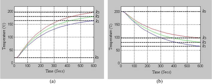
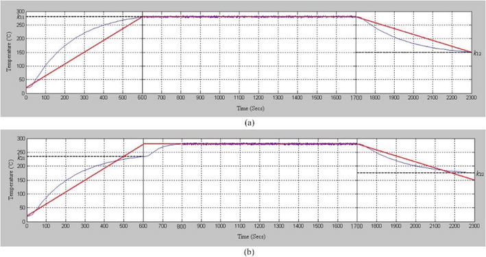
Passing through the preheating zone, the raw materials are slowly heated along with a moderate temperature rise trajectory, depending on the requirements of the physical initial properties of the product. Then, the temperature change of the materials depends on the time of passing through this zone and its temperature, which are determined by the set-point of the control system. When the preheating zone temperature is stabilized according to the set-point by PID control, the heat transfer characteristics of the raw material passing through this zone seem to be approximated by the first-order element with time delay from the step response experiment. Figure 1(a) shows the step response curve and the transfer function is equal to Eq. (1).

Figure 1.

Step responses. (a) Preheating zone. (b) Reducing zone.

$$G\left(s\right)=\frac{k}{\mathrm{Ts}+1}{e}^{-\mathit{\tau s}}$$E1

where T is the heat transfer time constant depending on the mass of the material, τ is the time delay, and k is the steady-state value.

As shown in Figure 1, the value of the steady-state k impacts on the reachable temperature at a certain period. The elapsed time of passing through the preheating zone also varies depending on the conveyor moving speed. Therefore, in order to satisfy the temperature reference trajectory of the raw materials, it is necessary to change the temperature set-point of this zone according to the conveyor speed. The heating zone is the most important one for ensuring the physicochemical properties of products. The color of products that reflects the primary quality requirements is changed sensitively by the temperature, conveyor speed and input material quantity in this zone. Therefore, to achieve the desired color of products, it is necessary to change the temperature and conveyor speed of this zone with the variation of material quantity. The conveyor speed of the kiln process is controlled to only satisfy the control characteristics of the heating zone under certain constraints, and the speed in the preheating and reducing zone is dependent on the heating zone.

In the reducing zone, the materials are cooled slowly along with the moderate temperature drop trajectory from the outlet temperature in the heating zone to meet the physical properties according to the product quality stabilization requirements. The temperature change of the materials depends on the temperature and passing time of this zone.

The temperature change of the materials and control requirement in this zone is the same as the preheating zone, but the only difference is that this is the cooling process due to the temperature drop. The heat transfer model is the same as for the preheating process and the step response is shown in Figure 1(b).

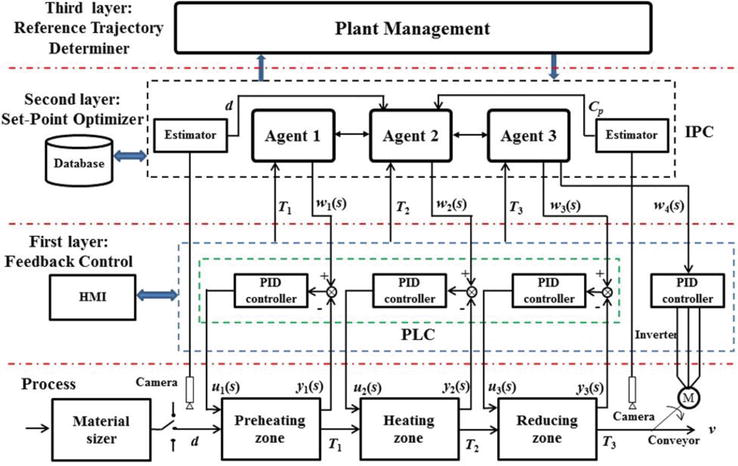
Each zone and conveyor of the kiln are controlled independently by a decentralized PID controller according to a given set-point, respectively. In Figure 2, the set-points are denoted as w₁(s), w₂(s), w₃(s), and w₄(s); manipulated variables as u₁(s), u₂(s) and u₃(s); the controlled variables as y₁(s), y₂(s) and y₃(s) and v, which respectively correspond to the temperature T₁, T₂ and T₃ and the conveyor speed. If the quantity of the material in the flow lines remains constant, the thermal equilibrium would be also maintained. If not, it is possible that the thermal balance in the kiln would be affected by the change in the material quantity. Therefore, the overall heat quantity of the materials is calculated as follows:

Figure 2.

Three-layer ISCS architecture.

$$\mathit{Qc}={\mathit{Qc}}_1+{\mathit{Qc}}_2+{\mathit{Qc}}_3\left(\mathrm{kJ}\right)$$E2

where Qc₁, Qc₂ and Qc₃ are the heat quantity of each zone.

Since the variation of the heat quantity due to the change of the material quantity causes the variation of the surface color of the products from kilns, it is unlikely that the color characteristics of the products would be stabilized by the control loops.

2.3 MPC: Set-point optimization

The two-layer structured ISCS, which employs the reinforcement learning method in which the agent learns through interaction with the environment, was developed to optimize the set-points of the temperature and speed controllers instead of the human operator in the heating zone [12].

The human operator empirically determines the set-points of the control loops in the original process and evaluates the input material quantity and the color of product images by using CCD cameras at the input and output of kiln processes. After that where set-points for the temperature and the conveyor belt speed in each zone are properly provided through HMI (Human Machine Interface) for maintaining the product color to the required value.

Due to the difficulty of considering all the variables in the operation of the real process, the human operator usually regulates set-points of the conveyor speed and the temperature for the heating zone to cope with the change of the material quantity, but not the temperature for the preheating and reduction zone. During the process operation, all values of process variables are stored in the database.

Moreover, considering the fuzziness of the human’s action for product stabilization, the following relationships between state and action variables would hold:

$$\text{IF}d=\mathrm{A}\text{and}v=\mathrm{B}\text{and}{T}_i={\mathrm{C}}_i\text{THEN}\Delta v=\mathrm{E}\text{and}\Delta T_i={\mathrm{F}}_i$$E3

where d (kg/m²) is the quantity of material, v (m/s) is the speed of the conveyor, T_i (°C) is the temperature of the heating zone and Δv and ΔT_i are the offset of the speed and the temperature set-points, and A, B, C_i, E and F_i are fuzzy sets.

The proposed three-layer structured ISCS consists of a distributed MPC system with several agents, in which the set-point optimizers of the second layer calculate the optimal set-points of the decentralized controllers to satisfy the control characteristics according to the product quality requirements in each zone with the reference trajectory provided by the economic optimization layer.

Agent 1 receives the temperature T₁ of the preheating zone and the conveyor speed v determined by agent 2 as stated and determines the temperature set-point change ΔT₁ of a controller in accordance with the quality requirements in this zone as an action. Thus, the action of agent 1 makes a decision to satisfy the economic efficiency by depending on the action of agent 2.

Agent 2 observes states such as speed v, temperature T₂ in the heating zone and the input material quantity d obtained by the estimator from CCD camera images, and then, it determines the optimal change of set-point Δv and ΔT₂ for speed and temperature of the controller to stabilize the output product color C_p. Agent 2 does not depend on the action of other agents, acts independently, and only provides its own action results upon their request.

Agent 3 receives the speed v and the temperature T₃ of the reducing zone as stated and determines the temperature set-point change ΔT₃ of the controller as an action to meet the quality requirements. The action of agent 3 also depends on the action of agent 2 as well as agent 1.

This system can be modeled as a multi-agent system, which is a group of single agents with independent subsystems. Reinforcement Learning is a powerful approach to solving multi-agent learning problems in complex environments.

This paper focuses on the design problem of multi-agent Q-learning for set-point optimization of controllers in the set-point optimization layer to solve the distributed NMPC problem, which approximates the temperature trajectory of materials to the reference trajectory in each zone.

The distributed NMPC problem is to determine the temperature set-point change ΔT_i and the speed set-point change Δv, which minimizes the following cost functions J_i(k) subject to constraints on input and output signals in each zone at the sampling time k:

$$J_1\left(k\right)=\sum _{p=1}^{L-1}{\left(r_1\left(k+p\right)-y_1\left(k+p\right)\right)}^2+\sum _{p=0}^{L-2}{\mathit{\Delta T}}_1{\left(k+p\right)}^2$$E4

$$J_2\left(k\right)=\sum _{p=L}^{M-1}{\left(r_2\left(k+p\right)-y_2\left(k+p\right)\right)}^2+\sum _{p=L-1}^{M-2}{\mathit{\Delta T}}_2{\left(k+p\right)}^2+\sum _{p=L-1}^{M-2}\mathit{\Delta v}{\left(k+p\right)}^2$$E5

$$J_3\left(k\right)=\sum _{p=M}^N{\left(r_3\left(k+p\right)-y_3\left(k+p\right)\right)}^2+\sum _{p=M-1}^{N-1}{\mathit{\Delta T}}_3{\left(k+p\right)}^2$$E6

where N is the total predicted length (p = 1, 2, ..., N), y_i is the temperature prediction trajectory of materials and r_i is the reference trajectory. That is, NMPC is formulated as the optimal control problem with the objective function as follows:

$$minJ\left(k\right)=\sum _{i=1}^3{J}_i\left(k\right)$$E7

subject to:

$$\begin{array}{c}{T}_{i,min}\le T_i\left(k\right)\le T_{i,max}\\ \Delta T_{i,min}\le \Delta T_i\left(k\right)\le \Delta T_{i,max}\\ v_{\min }v\left(k\right)v_{\max }\\ \Delta v_{\min }\Delta v\left(k\right)\Delta v_{\max }\\ y_{i,min}\le y^i\left(k\right)\le y_{i,max}\end{array}$$E8

With constraints, the cost functions can be minimized numerically by the optimal action of agents.

2.4 Operational objectives determination

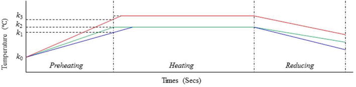
The third layer functions as the plant control layer, where the optimal reference trajectory would be calculated to achieve the economic effectiveness of the process according to its operational objective determined by the quality requirement of the product. The obtained reference trajectory would be provided to the decentralized agents. Figure 3 shows three typical reference trajectories determined according to the operating objectives of the quality requirements in each zone.

Figure 3.

The reference trajectories for three-step kiln process.

3. Design of Q-learning agents for online set-point optimization

This section describes the design of the decentralized Q-learning agents for set-point optimization of controllers in each zone to solve the distributed NMPC problem.

3.1 Q-learning and multi-agent

From the analysis of references [13, 14], Q-learning is described as follows [12].

The Q-learning algorithm is a model-free reinforcement learning method and its convergence has been proved. The Q-learning estimates the expected value Q^*(s, a) of the discounted reward sum as Q-value through randomized interactions with the environment without the requirement of knowledge for transition probabilities in Markov decision process (MDP).

The action value Q(s, a) is the estimate of an action a in a state s and its updating process would be recorded in a Q-table. Generally, the initial value of the Q(s, a) called Q-function is given randomly and is approximated iteratively to the optimal Q-function. As a state transits from s_t to s_t + 1 by an action a, the agent updates Q(s_t, a_t) as follows:

$$Q\left(s_t,a_t\right)\Leftarrow \left(1-\alpha \right)Q\left(s_t,a_t\right)+\alpha \left[r_{t+1}+\gamma \underset{a}{max}Q\left(s_{t+1},a\right)\right]$$E9

where α ∈ (0, 1] is the learning rate, r_t + 1 the immediate reward for the next state s_t + 1 and max_aQ(s_t + 1, a) the maximum action value in the same state. The Q-learning algorithm for estimating Q^*(s, a) is given in Table 1.

Set the initial value of Q(s, a) randomly and t = 0. Measure the current state st. Determine an action at from st using policy given in Q-table. Apply action a, measure next state st + 1 and reward rt + 1. Update Q(s, a) by Eq. (9). t ← t + 1. Repeat from step 2 until convergence.

Table 1.

Q-learning algorithm.

The Q-table can be utilized as a dynamic model of the environment after the learning has been completed because it reflects the dynamic characteristic of the environment.

Despite the effectiveness for optimal policy, the Q-learning algorithm has some drawbacks of slow convergence. To tackle these issues, problem definition, discretization and learning parameters should be properly determined in practical circumstances [15].

It is usually difficult for a single agent to implement a large-scale complex task due to its own limited capacity. Multi-agents, which collaborate agents with each other through decentralized computation, can greatly improve their solving efficiency. However, since multi-agent learning process is quite complex, it is not so simple to solve cooperative problem of single agents.

The cooperative control problem of decentralized multi-agents for complex objects that cannot be solved by a single agent has been studied [16, 17, 18].

Although multi-agent systems are effective in large-scale complex environments, many difficulties remain in their solution methods.

3.2 Agent design for heating zone

The heating zone is the most important part for the quality of products, and the agent for the determination of the controller set-point in this zone does not depend on the action of the other agents, but only transmits its future action through the message with the request of other agents. Thus, the agent design in this zone becomes the single agent problem. The materials passing through this zone cause physicochemical changes and are calcined near the appropriate temperature set-point for a certain time.

Although the temperature in this zone is at a steady state, the temperature trajectory of materials cannot be properly predicted by the heat transfer model because the input material quantity changes the variation of the heat quantity of materials. Hence, in order to stabilize the heat quantity that materials receive, the agent evaluates the color of the output product and determines the optimal set-point change Δv and ΔT₂ of the temperature and conveyor speed for the heating zone controller according to Eq. (3) in each action cycle. Thus, Eq. (5) is reformulated as follows:

$$J_2\left(k\right)=\sum _{p=L}^{M-1}{\left(r_{\mathrm{cp}}\left(k+p\right)-y_{\mathrm{cp}}\left(k+p\right)\right)}^2+\sum _{p=L-1}^{M-2}{\mathit{\Delta T}}_2{\left(k+p\right)}^2+\sum _{p=L-1}^{M-2}\mathit{\Delta v}{\left(k+p\right)}^2$$E10

where r_cp is the desired reference luminance of the product, and y_cp is the measured luminance obtained in the estimator.

The agent designing for the heating zone involves the designing of the state space, action space and reward function as in [12] (see Appendix A).

3.3 Cooperative agent design for preheating and reducing zones

Like single-agent reinforcement learning, multi-agent reinforcement learning is also based on MDP as a formalization of multi-agent interaction. Agents act collectively and cooperate to achieve their own individual goals as well as the common goal of the group to which they belong. However, each agent often cooperates with the other to achieve their own individual goals rather than solving a common problem.

In fact, since all the agents make their decisions simultaneously, each agent cannot recognize the others’ choices in advance, but make a choice to possibly transit from its current state to a better state. Therefore, the paper proposes multi-agent Q-learning as a form of joint state and individual action.

Preheating and reducing are the processes to satisfy the physical properties according to the specific quality requirements of the product. In each zones, agents 1 and 3 predict the temperature change y_i of the material according to the current temperature T_i (i = 1, 3) and the conveyor speed v in each action cycle using the step response model over the prediction horizon and calculate the optimal set-point changes of the controllers from Eq. (4) and (6) to approximate them to the reference trajectory r_i, respectively.

Since the conveyor velocity v is determined by the heating zone agent 2, the action of agents 1 and 3 depends on the action of agent 2. That is, the Q-learning agents act to maximize the reward based on the cooperative information with agent 2 and the independent interaction with the sub-environment. The agent’s action is represented by the following fuzzy rules:

$$\text{IF}v=\mathrm{B}\text{and}{T}_i={\mathrm{C}}_i\text{THEN}\Delta T_i={\mathrm{F}}_i,i=1,3$$E11

where B, C_i and F_i are fuzzy sets of physical quantities corresponding to linguistic evaluation.

3.3.1 State space

From Eq. (11), states of the preheating and reducing zones are the joint state of the state v of agent 2 and a state T_i of agent i (i = 1, 3). The continuous state variables v and T_i are discretized and the state space is partitioned into fuzzy subspaces that are assigned to five linguistic variables, respectively. The discrete joint state space can be represented as follows:

$$S=\left\{s|s_{\mathit{jk}}=\left(v_j,T_{i,k}\right),i=1,3,j=1,2,\dots ,J,k=1,2,\dots ,K\right\}$$E12

where J = K = 5 and the number of possible states are 5² = 25 and the triangular membership functions are used.

3.3.2 Action space

As shown in Eq. (11), the set-point change ΔT_i of controllers is the action variable of the agents for the operation of the preheating and reducing zones. The range of this variable is determined by ΔT_i ∈ [−15, +15] (°C) as the heating zone. The continuous action space is partitioned into fuzzy subspace which is assigned to five linguistic variables. The discrete action space for the agent is represented as follows:

$$A=\left\{a|a_m=\Delta T_{i,m},i=1,3,m=1,2,\dots ,M\right\}$$E13

where M is the number of equally divided fuzzy subset in the proper range of ΔT_i,m.

In each time step, based on the observed states (i.e. v_j and T_i,k) and the ε-greedy policy, the agents choose a state-action pair from Q-table and update the temperature set-points of control systems for speed and temperature for the preheating and reducing zones. By the action of agents, the temperatures are updated as follows:

$$T_i\left(t+1\right)=T_i\left(t\right)+\Delta T_i\left(t+1\right),i=1,3$$E14

3.3.3 Reward function

The action of agents in the preheating and reducing zones to meet the specific quality requirements of the product is guaranteed by approximating the heat transfer trajectory of the material passing through these zones to the reference trajectory. Thus, the reward signal of Q-learning for the control of these zones can be expressed as the inverse of the square sum of the deviation between the reference trajectory and the prediction trajectory over the prediction horizon, which is obtained by the set-point change at the current sampling time as follows:

$$r_{t+1}=\frac{1}{{\sum }_{k=0}^K{\left(r_i\left(k\right)-y_i\left(k\right)\right)}^2},i=1,3$$E15

where k is the prediction length in the ith zone and ${\sum }_{k=0}^K{\left(r_i\left(k\right)-y_i\left(k\right)\right)}^2>0$.

4. Q-learning convergence improvement

This section describes the convergence improvement of Q-learning agents designed above. Firstly, the results of our study on how to improve the convergence of Q-learning in the heating zone are presented. Next, to improve the convergence of Q-learning in the preheating and reducing zones, the initialization method of Q-table using the model is described.

4.1 Convergence improvement method of Q-learning using operational data

Methods for improving the convergence of Q-learning with discrete action as the primary acting mode are largely divided into tuning the learning parameters and fast updating of the Q-table.

In the heating zone, the convergence improvement method [12] of the Q-learning agent based on the method of obtaining the optimal Q-table is presented in Appendix B, but a brief outline is as follows.

The use of the agent in process operation has not been permitted until the learning is completed, because the heating zone agent uses a model-free Q-learning method that finds the optimal policy without prior knowledge of the environment.

Therefore, the method for improving the convergence of Q-learning is to determine the initial values of the Q-table optimally. This requires knowledge of the environmental dynamics, which is not easily obtained in the non-linear system.

The proposed method is realized by extracting automatically the operational experience rules of the expert from past operating data and initializing the Q-table using it.

4.2 Q-table initialization using model

In the zones for preheating and reducing of the calcined raw material, agents interact with the environment and adjust the set-point of the control systems according to the conveyor speed change, considering the cooperative information provided by the heating zone agent.

Taking into account the arbitrary variation of the speed, the agent action of determining the set-point change with the temperature of its zone is represented by a fuzzy logic rule as Eq. (11). When two state variables and one action variable have five fuzzy variables, respectively, the Q-table consists of 125 state-action pairs where the number of states is 25 and each state has 5 actions, respectively.

In the preheating and reducing zones, the heat transfer dynamics of the material from the step response experiment are shown in Figure 1. Given the dynamics, it is possible to perform the offline simulation.

This subsection presents a method of determining the optimal initial value of the Q-table using the dynamics model. Given the conveyor speed v determined by the action of the heating zone agent, the time t of passing through the zone can be calculated.

Based on the numerical simulation using the step response model, moreover, the set-point change where the heat transfer trajectory of the material is approximated to the reference trajectory can be determined repeatedly.

First, the initial Q-value is set to 0 and the reward is determined by the off-line simulation using the step response model and Eq. (15).

Eq. (15) is the reward function at a joint state S and an individual action A of agent i, that is,

$$R_i:S\times A\to \mathbf{R}$$E16

where R is the set of real numbers. Table 2 shows the structure of rules.

Rule	Description
R1	x1 = NB & x2 = NB & y = PB ⇨ Q = 9.8
R2	x1 = NB & x2 = NM & y = PM ⇨ Q = 7.6
R3	x1 = ZO & x2 = ZO & y = ZO ⇨ Q = 11.2
...	...
R125	x1 = PB & x2 = PB & y = NB ⇨ Q = 1.4

Table 2.

Structure of rules.

5. Results and discussion

The simulation result to evaluate the performance of the agent for the heating zone is presented in Appendix C.

The simulation result for the preheating and reducing zones does not present because there have already existed the explicit heat transfer models in these zones, but only the operating experiment result.

During the operation experiment, firstly, the luminance of the output product is utilized to compare the operation by the human with the agent for the heating zone [12].

It is usually impossible to run the comparative experimentation with the traditional method in a real situation due to the trial-and-error features in the Q-learning with arbitrarily initialized Q-value. Therefore, the operations of an operator are preferred to evaluate the proposed method.

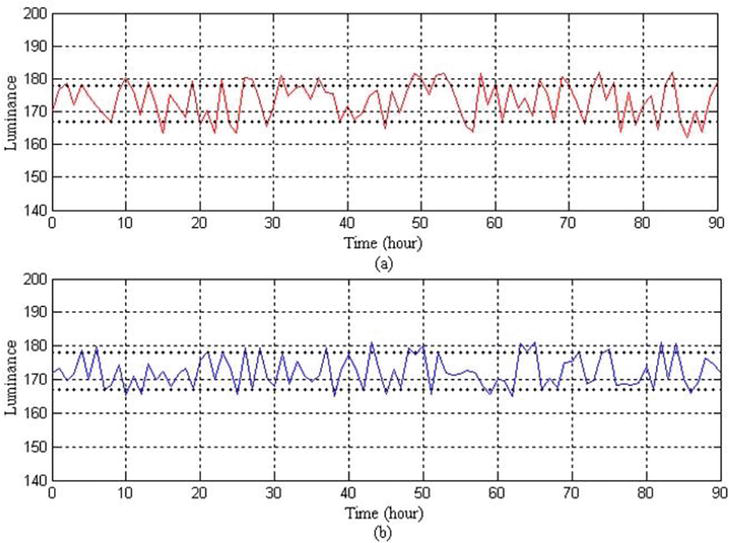
Figure 4 shows the comparison results for 90 hour-experiment.

Figure 4.

Operation experiment result of real process. (a) Operation by human operator. (b) Operation by agent.

The tolerance limitation Y₀ of luminance lies between 167 and 178. The luminance Y for the manual operation changes within the range of Y₀ ± 5 and its deviation V is 0.4%. For the proposed case, the experiment results are that Y=Y₀ ± 3 and V = 0.4%.

In spite of the sub-optimality of the initial Q-values, it seems that the convergence feature was mostly satisfied.

However, the experiment for human operation shows somewhat insufficiency. The operator’s experience might have a decisive impact on the long-term operation. Furthermore, it is unlikely that human might always make the correct decision for set-points of control systems.

From the above results, it is certain that the proposed method improves the trial-and-error features in the Q-learning with arbitrarily initialized Q-value.

Next, in the preheating and reducing zones, the online set-point determination method using the cooperative action of agents is compared with the previous method by the deviation between the predicted temperature trajectory and the reference trajectory.

Figure 5 shows the results of an experiment for the comparison of the temperature change trajectory with the reference trajectory according to the operating mode of the kiln process. Since the temperature trajectory of the material in the heating zone cannot be predicted by the heat transfer model, the medium part of the plot for this zone demonstrates the relative change of the heat quantity estimated by the luminance of the product during the experiment.

Figure 5.

Comparison of temperature change trajectory approximation. (a) Previous method. (b) Improved method.

In the previous approach, the supervisory control by the intelligent agent was implemented for the heating zone with the temperature of the preheating and reducing zones being constant due to the operational complexity. In this operational mode, the reference trajectories and the predicted temperature trajectories are shown in Figure 5(a).

On the other hand, Figure 5(b) demonstrates the temperature trajectories improved by the optimal set-point control in the operational mode with the cooperative action of decentralized agents to meet the high-quality requirement.

Moreover, in the case of batch production for a limited amount of specific product, it is possible to satisfy the more accurate temperature trajectory by stepwise change of the set-point.

Experimental results show that the cooperative action of agents for determining the set-point of the decentralized local controllers ensures the economic optimization of the process operation.

6. Conclusions

This paper proposes an NMPC design problem with the hierarchical structure as an online set-point optimizer to maximize the economic efficiency of long-term operation in order to meet the strict quality requirements of products in the cascaded three-step kiln.

Firstly, a three-layer ISCS was designed, which involves a direct control layer for the kiln process, an online set-point optimization layer for decentralized controllers and a management layer for the economic optimization of the process.

Second, a distributed MPC system that approximates the temperature trajectory of the raw material of passing through the kiln to an integrated reference trajectory is proposed, which adopts the multi-agent Q-learning to optimize the set-point for decentralized controllers.

Third, a new method for fast Q-learning convergence is proposed. For the agent of the heating zone, the human operator’s experience rules were automatically extracted from the process database using C4.5, and the Q-table initialization algorithm based on experience rules was developed.

In addition, for agents of the preheating and reducing zones, the Q-table initialization method using the model is proposed.

Thus, the cooperative action of multi-agent Q-learning-based ISCS determines the optimal set-points of the controllers to stabilize the process, so that it can replace the human operator in the kiln process which does not permit the trial-and-error operations. Moreover, the experiments show that fast Q-learning convergence is guaranteed by the proposed method.

This method has great significance in designing the supervisory control system for complex processes such as the ceramics, the foodstuff and the paper industry. Our future work considers the optimization problems at the plant management layer of the hierarchical MPC systems.

A.1 State space

If the temperature trajectory in the preheating and reducing zones of Figure 2 are satisfying the reference trajectory, the relation between the material quantity d, the speed v, the heating zone temperature T₂ and the product color C_p can be represented as follows:

$$\left(d,v,T_2\right)\to C_p$$E17

where v and T₂ are measured by the controllers (PLCs) and d and C_p are calculated as the luminance through the estimator from the CCD camera image. In order to represent the grey-scale information by the luminance Y from the 8-bit RGB color model, the YIQ color model [19] is used as follows:

$$Y=0.299R+0.587G+0.114B,Y\in \left[0,255\right]$$E18

d is given as the percentage of the white-colored- material area to the black-colored-belt area in the unit area from the two-value black-white image, which is converted from the grey-scale image. The state variables d, v and T₂ are discretized so that Q-learning agent could determine the optimal set-point for the speed and temperature by the iterative algorithm to meet the luminance requirement of product under the variation of the material quantity.

The state space is partitioned into fuzzy subspaces represented by five linguistic variables, that is (NB, NM, ZO, PM, PB), which can be represented from Eq. (17) as follows:

$$S=\left\{s|s_{\mathit{ijk}}=\left(d_i,v_j,T_{2,k}\right),i=1,2,\dots ,I,j=1,2,\dots ,J,k=1,2,\dots ,K\right\}$$E19

where I, J and K are the numbers of equally divided fuzzy subsets in the proper ranges of d_i, v_j and T_2,k, respectively, I = J = K = 5 and the number of possible states are 5³ = 125.

A.2 Action space

In Figure 2, the set-point change, Δv ∈ [−0.02, +0.02] and ΔT₂ ∈ [−15, +15] (°C), are the action variables of the agent for the preheating zone and the action space is partitioned into the fuzzy sub-spaces denoted by five linguistic variables as follows:

$$A=\left\{a|a_{\mathit{lm}}=\left(\Delta v_l,\Delta T_{2,m}\right),l=m=1,2,\dots ,5\right\}$$E20

The number of possible actions for each state (d, v, T₂) is 5² = 25. The agent chooses a pair of state-action from Q-table based on the observed states and the ε-greedy policy of choosing actions.

According to this, the rules for updating set-points for the speed and the temperature are as follows:

$$v\left(t+1\right)=v\left(t\right)+\Delta v\left(t+1\right)$$E21

$$T_2\left(t+1\right)=T_2\left(t\right)+\Delta T_2\left(t+1\right)$$E22

where v(t + 1) and T₂(t + 1) are the speed and temperature set-points in the present time, v(t) and T₂(t) are ones in the past time, respectively.

A.3 Reward function

Since the product color C_p as the quality characteristic depends on the d, v and T₂, the luminance is used as the reward of the reinforcement learning for the heating zone.

Due to the action of the agent, the state s_t proceeds to s_t + 1 and the product color C_p(t) changes to C_p(t + 1). The reward r_t + 1 given to the agent is as follows:

$$r_{t+1}=f\left(C_p\left(t+1\right)\right)$$E23

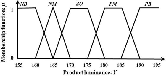
Considering the experimental results, the luminance value of Eq. (18) is partitioned into five fuzzy sets, as shown in Figure 6, and Eq. (23) is defined as the discrete reward function such as Eq. (24).where the value of Y′ is the fuzzy variable for the linguistic evaluation of the luminance Y.

$$r_{t+1}=\left\{2,Y^{\prime }=\mathrm{ZO}|\right.\left\{1,Y^{\prime }=\mathrm{PM}|\right.\left\{0,Y^{\prime }=\mathrm{NM}|\right.\left\{-1,Y^{\prime }=\mathrm{PB}|\right.\left\{-2,Y^{\prime }=\mathrm{NB}|\right.$$E24

Figure 6.

Fuzzy set of luminance value.

The scheme of improving the Q-learning convergence for the heating zone agent involves procedures such as (i) Extracting the decision tree for the operational experience rules from the historical database, (ii) Converting the decision tree to fuzzy rule, (iii) Initializing the Q-table by the fuzzy rule.

B.1 Extraction of operating rules from data

B.1.1 Extraction of instances set

The data records R(At₁, At₂, …, At_k, ...) stored in the database involves the state variable set X = {x₁, x₂, ..., x_k}, the action variable set (set-points) Y = {y₁, y₂, ..., y_p}, the operator’s experience knowledge and the process dynamics.

Thus, the new relationship between the state and action is obtained using the relational projection operation [20] as follows:

$${\prod }_q\left(R\right)=\left\{t\left[q\right]|t\in R\right\}$$E25

where t[q] is the set of the value of the attribute q to the element t of the relation R.

First, samples are selected from the created relations and each element of the sample is normalized onto the interval [0, 1]. And the normalized samples are classified according to the Euclidean similarity criteria of Eq. (26) and the obtained instances are classified randomly into training data and test data:

$$r_{\mathrm{ij}}={\left[\sum _{k=1}^m{\left(q_{\mathrm{ik}}-q_{\mathrm{jk}}\right)}^2/m\right]}^{1/2}$$E26

where q_i = (q_i1, q_i2, …, q_im) and q_j = (q_j1, q_j2, …, q_jm) are ith and jth samples.

The obtained instance set D consists of two classes according to the value C of class that if the luminance which shows the product quality lies in the proper range δ then C = 1 else C = 0, and its structure is shown in Table 3. Then, D₁ ∩ D₀ = ϕ.

	I1	I2	I3	…	Im	Class
1	x11	x12	x13		x1m	C1
2	x21	x22	x23		x2m	C2
3	x31	x32	x33		x3m	C3
…	…	…	…	…	…	…
n	xn1	xn2	xn3		xnm	Cn

Table 3.

Structure of instance set.

In Table 3, the attribute set I = {I₁, I₂, ..., I_m} contains the state variable set X and the action variable set Y, where I = X ∪ Y, X ∩ Y = ϕ and m = k + p.

B.1.2 Rule generation

The decision tree learning method to extract the operating rules from data utilizes the C4.5 algorithm [21], which is the successor of ID3 [22].

C4.5 algorithm for constructing the decision tree includes the following contents:

1. To choose the root node.

2. To construct the branches based on every value of the root node.

3. To continue the construction of the decision tree until no further disintegration occurs to the attributes.

The fuzzification of attributes is conducted to extract the fuzzy rules such as Eq. (27) from Table 3.

$$\text{Rule}{R}_j:\text{If}{x}_1\text{is}{A}_{j1}\text{and}\dots \text{and}{x}_m\text{is}{A}_{\mathit{jm}}\text{then class}{C}_j,j=1,2,\dots ,N$$E27

where X = [x₁, x₂, ..., x_m] is the m-dimensional sample vector, A_ji (i = 1, 2, ..., m) is the fuzzy set of x_j; C_j ∈ {0, 1} is the pattern class of the jth rule and N is the number of fuzzy rules.

In the decision tree constructed from the training data by the C4.5 algorithm, each path from a root to a leaf represents a rule.

Table 4 shows some rules obtained from the decision tree.

Rule	Description
R1	x1 = NB & x2 = PM & x3 = ZO & y1 = PB & y2 ZO ⇨ C = 1
R2	x1 = PM & x2 = PM & x3 = ZO & y1 = ZO & y2 = PM ⇨ C = 1
R3	x1 = ZO & x2 = PM & x3 = ZO & y1 = NB & y2 = PM ⇨ C = 0
R4	x1 = NB & x2 = PM & x3 = ZO & y1 = NB & y2 = PM ⇨ C = 0
R5	x1 = ZO & x2 = ZO & x3 = ZO & y1 = ZO & y2 = ZO ⇨ C = 1

Table 4.

Some of the decision tree rules.

B.1.3 Obtaining of state-action rules

The state-action pairs with the C = 1 in Table 4 represent the operating conditions applicable to the process. Therefore, by choosing only the rules with C = 1 among the N rules, the fuzzy rules for the following state-action pairs would be obtained:

$$\text{Rule}{R}_k:\text{If}{x}_1\text{is}\mathrm{NM}\text{and}{x}_2\text{is}\mathrm{NM}\text{and}{x}_3\text{is}\mathrm{NM}\text{then}{y}_1\text{is}\mathrm{NM}\text{and}{y}_2\text{is}\mathrm{PM}$$E28

where k = 1, 2, ..., M is the number of rules and M < N.

B.2 Initialization method of Q-table

From Eq. (28), as each rule has 3 fuzzy variables for state and 2 fuzzy variables for action, the Q-table contains 125 states, each of which has 25 actions.

However, since only the empirical knowledge of operator is stored in the process database, the fuzzy rule obtained from Table 4 reveals only the most appropriate action to the given state among the possible action space.

Thus, we propose the algorithm of initializing the Q-value for the action space that cannot be obtained by the decision tree for each state in Table 5.

i = 1. Search the rule of Eq. (28), whose antecedent matches the ith state si in Q-table. If the rule does not exist, then go to step 5. Assign maximum value to the Q-value of an action that matches with the consequence of the rule. Initialize Q-values of the rest actions using Eq. (31) and go to step 6. Initialize Q-values of all possible actions to the state si as zero. i ← i + 1. Repeat from step 2 for all the states.

Table 5.

Initialization algorithm of Q-table.

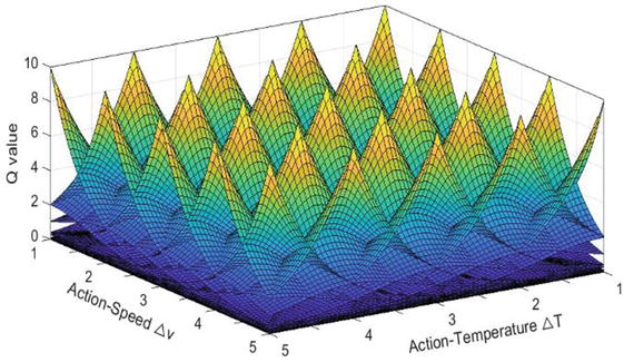
The exponential function distribution used in the determination of Q-values in the three-dimensional space is represented as follows:

$$Q_0\left(w_1,w_2\right)=A·exp\left(-k\Vert \mathrm{w}-\mathrm{r}\Vert \right)$$E29

where ||w-r|| is the Euclidean Square Norm of feature vectors defined as follows:

$$\Vert \mathrm{w}-\mathrm{r}\Vert ={\left(\sum _l^n\left({\left|w_l-r_l\right|}^2\right)\right)}^{1/2}$$E30

Since n = 2, the function for initializing Q-value is represented as follows:

$$Q_0\left(w_1,w_2\right)=A·exp\left(-k{\left({\left(w_1-r_{1i}\right)}^2+{\left(w_2-r_{2j}\right)}^2\right)}^{1/2}\right),\left(w_1,w_2\right)\in W$$E31

where actions w₁ and w₂ have the values of Δv and ΔT, respectively, W is the action set and i = j = 1, 2, …, 5. r_1i and r_2j are respectively the centres of the ith and jth action range. A is the initial constant value and k is the growth constant. In this study, A = 10 and k = 1.6, respectively.

The function plotted in MATLAB is shown in Figure 7.

Figure 7.

Assignment of Q-value in 5 × 5 action space.

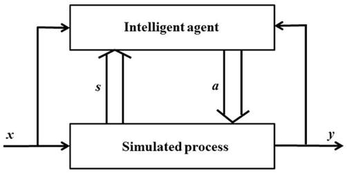
Figure 8 shows the architecture of the simulation system, which is used to evaluate the performance of the agent for the heating zone under the assumption that the direct control layer in Figure 2 performs well enough.

Figure 8.

Architecture of simulation system.

The reward for the agent is calculated by Eq. (24) and the reward signal is simulated by the following luminance prediction model corresponding to the color of product obtained using the process data:

$$y=170.34+5.97x_1+2.87x_2-0.894x_3$$E32

where x₁, x₂, x₃ and y denote the quantity of material d, the speed v, the temperature T and the product luminance Y, respectively. Thus, the agent observes the states of the process through x₁, x₂ and x₃, and takes the actions through Δx₂, Δx₃, and estimates the reward by y. During simulation, the Q-table and parameters for the real process are utilized (Table 6).

Parameter	Variable	Value	unit
Learning rate	α	0.1
Discount factor	γ	0.9
Material quantity	d	10 ∼ 50	%
Belt speed	v	3 ∼ 7	m/min
Temperature	T	180 ∼ 340	°C
Luminance	Cp	155 ∼ 195

Table 6.

Parameters for simulation.

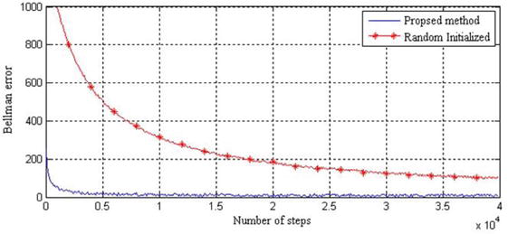
The simulation and experiment results are shown in Figures 9–11.

Figure 9.

Comparison of Q-learning convergence.

Figure 10.

Simulation results of quality characteristics. (a) Input quantity change. (b) Initialized method arbitrarily. (c) Proposed method.

Figure 11.

Comparison of average reward.

Figure 9 compares the Q-learning convergence of the proposed method to the traditional one in regard to the Bellman error [23].

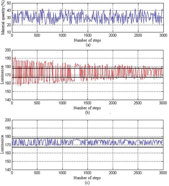
Figure 10 demonstrates the operating characteristic during simulation.

In Figure 10(a), the virtual input x₁ changes randomly and the variables x₂, x₃ are given as certain values according to the process.

In Figure 10(b) and (c), the upper and lower limit of the luminance corresponding to the product quality is shown as the thick line.

The luminance is calculated by Eq. (32) and the reward is predicted by Eq. (24).

The deviation of luminance is V = 5.66% for the traditional method, whereas V = 0 during learning iterations for the proposed method.

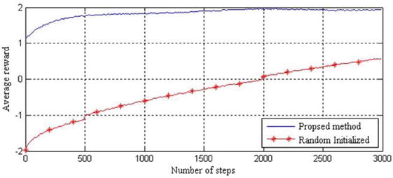
Figure 11 shows the comparative result of the proposed method with the random initialized one by the average reward method [14].

Simulation results show that the proposed method satisfies the Q-learning convergence and the function optimality in the initial learning phases.

References

1.Fekri S, Assadian F. Fast model predictive control and its application to energy Management of Hybrid Electric Vehicles. In: Zheng T, editor. Advanced Model Predictive Control. London, UK: IntechOpen; 2011. pp. 3-28 ch1
2.Ocampo-Martinez C. Model Predictive Control of Wastewater Systems. Springer-Verlag London Limited; 2010. p. 216. DOI: 10.1007/978-1-84996-353-4
3.Wang L. Model Predictive Control System Design and Implementation Using MATLAB®. Springer-Verlag London Limited; 2009. p. 374. DOI: 10.1007/978-1-84882-331-0
4.Qin SJ, Badgwell TA. A survey of industrial model predictive control technology. Control Engineering Practice. 2003;11(7):733-764
5.Arellano-Garcia H, Barz T, Dorneanu B, Vassiliadis VS. Real-time feasibility of nonlinear model predictive control for semi-batch reactors subject to uncertainty and disturbances. Computers and Chemical Engineering. 2020;133:1-18. DOI: 10.1016/j.compchemeng.2019.106529
6.Patil BV et al. Decentralized nonlinear model predictive control of a multi-machine power system. Electrical Power and Energy Systems. 2019;106:358-372. DOI: 10.1016/j.ijepes.2018.10.018
7.Zhang A, Yin X, Liu S, Zeng J, Liu J. Distributed economic model predictive control of wastewater treatment plants. Chemical Engineering Research and Design. 2019;141:144-155. DOI: 10.1016/j.cherd.2018.10.039
8.Brdys M, Tatjewski P. Iterative Algorithms for Multilayer Optimizing Control. London, UK: Imperial College Press; 2005. p. 370
9.Marusak P, Tatjewski P. Actuator fault toleration in control systems with predictive constrained set-point optimizers. International Journal of Applied Mathematics and Computer Science. 2008;18(4):539-551. DOI: 10.2478/v10006-008-0047-2
10.Tatjewski P. Supervisory predictive control and on-line set-point optimization. International Journal of Applied Mathematics and Computer Science. 2010;20(3):483-495. DOI: 10.2478/v10006-010-0035-1
11.Li H, Swartz CLE. Dynamic real-time optimization of distributed MPC systems using rigorous closed-loop prediction. Computers and Chemical Engineering. 2018;122:356-371
12.Kim SH, Song KR, Kang IY, Hyon CI. On-line set-point optimization for intelligent supervisory control and improvement of Q-learning convergence. Control Engineering Practice. 2021;114:104859. DOI: 10.1016/j.conengprac.2021.104859
13.Watkins CJCH, Dayan P. Technical note: Q-learning. Machine Learning. 1992;8:279-292
14.Montague PR. Reinforcement Learning: An Introduction, by Sutton RS, Barto AG. Trends in Cognitive Science 3, no 9; 1999. p. 360
15.Zarrabian S, Belkacemi R, Babalola AA. Reinforcement learning approach for congestion management and cascading failure prevention with experimental application. Electric Power Systems Research. 2016;141:179-190. DOI: 10.1016/j.epsr.2016.06.041
16.Chen X, Chen G, Cao W, Wu M. Cooperative learning with joint state value approximation for multi-agent systems. Journal of Control Theory and Applications. 2013;11(2):149-155. DOI: 10.1007/s11768-013-1141-z
17.Wang H, Wang X, Hu X, Zhang X, Gu M. A multi-agent reinforcement learning approach to dynamic service composition. Information Sciences. 2016;363:96-119. DOI: 10.1016/j.ins.2016.05.002
18.Zemzem W, Tagina M. Cooperative multi-agent systems using distributed reinforcement learning techniques. Procedia Computer Science. 2018;126:517-526. DOI: 10.1016/j.procs.2018.07.286
19.Girgis MR, Mahmoud TM, Abd-El-Hafeez T. An approach to image extraction and accurate skin detection from web pages. International Journal of Electrical and Electronics Engineering. 2007;1(6):353-361
20.Codd EF. The Relational Model for Database Management: Version 2. Menlo Park: Addison-Wesley Publishing Company; 1990. p. 538
21.Quinlan JR. C4.5: Programs for Machine Learning. San Francisco: Morgan Kaufmann Publishers; 1993
22.Quinlan JR. Induction of decision trees. Machine Learning. 1986;1(1):81-106
23.Buşoniu L, Babuška R, Schutter B, Ernst D. Reinforcement Learning and Dynamic Programming Using Function Approximators. Boca Raton: CRC Press; 2010. p. 267
Written By
Song Ho Kim and Kwang Rim Song
Submitted: 03 January 2023Reviewed: 10 January 2023Published: 12 July 2023
Open access peer-reviewed chapter