Review of Model Predictive Control and Other Methodologies for Lateral Control of an Autonomous Vehicle

Abstract

This chapter summarizes controller methodologies for lateral control of a standard passenger vehicle, with front-wheel steering and fixed rear wheels. Comparisons are made to elucidate benefits and drawbacks of the application of a model predictive controller. Select widely used system models are described, and a general problem formulation for the model predictive controller is given. Two publicly available examples of this application are reviewed and compared, and the results are discussed.

1. Introduction

Automatic navigation and control of terrestrial vehicles are a rapidly growing and developing field, with a wide range of applications. From meal-serving robots in restaurants to GPS-localized tractors that can till fields without human interaction, the potential for this domain of research and application in industry is only recently being expanded. Recent advances in computational, sensory, and battery technologies have enabled the automation of perhaps the most popular domain, automotive systems. The automotive industry has a long history of utilizing feedback control systems, in functions such as cruise control for longitudinal control and lane-keeping assistance for lateral control. In fact, control of an autonomous vehicle has historically been decomposed into these two categories – longitudinal and lateral control. However, in order to achieve higher levels of autonomy, it is vital to develop a control framework that generates a high-quality coordinated response between both vehicle states. In this chapter, a comparison between the various control schema will be illustrated to weigh the pros and cons of a model predictive controller in this application. For the use of an MPC system in simulation, it will be necessary to compare several models, MPC formulations, and optimization methods. At the end of this chapter, one example of such a controller will be presented for both a linear and nonlinear case to illustrate the performance and capabilities of such a controller, as well as the advantages and disadvantages, which come with its implementation.

2. Controller review

In the application of automotive controllers, virtually all inputs can be described as a combination of a yaw steering input produced by the steering wheel, and a velocity target input produced by the accelerator pedal. There do exist some controllers that can utilize torque vectoring or incorporate additional actuators to the system to add an additional degree of freedom, but these will not be addressed in this chapter as they require equipment not found on the vast majority of passenger vehicles. Controllers can be categorized in several ways, and for simplicity’s sake will be compared within three major categories: geometric, frequency domain, and state-space formulated controllers. Controllers in the latter two categories have some overlap, in that linear controllers can almost always be described in both a state-space and frequency domain representation; the distinction in this section is made to provide a concise description of the different methodologies. This chapter will focus on the lateral control of a standard passenger vehicle but will include consideration for longitudinal control where relevant and applicable. Controllers are usually given a reference trajectory, which is the desired path for the vehicle to take and must extract the useful information from this path and the vehicle’s relative pose to generate the controller outputs.

2.1 Geometric controllers

Geometric controllers simply use the geometric and kinematic relations of the vehicle to generate an output. In lateral control, the most popular formulations are the pure-pursuit and Stanley controllers.

2.2 Pure-pursuit

Perhaps the most simple controller that sees real-world use, a pure pursuit controller uses some look-ahead distance to generate a steering output. In the most simple application, a fixed distance is selected, and a point on the target trajectory path at this distance from the car is used to determine the steering output. The output steering is directly proportional to the yaw angle of this geometric link. Additional complexity can be added by having this look-ahead distance vary as vehicle speed changes. This works well in simple, low-curvature environments but has no claims of optimality or robustness. Furthermore, as the vehicle approaches a path, such as a straight line or slight curve, it will asymptotically approach the line even in ideal circumstances. Additional logic needs to be included to improve target following and account for situations where the car is further away from the path than the look-ahead distance.

2.3 Stanley

The Stanley controller is a more advanced geometric controller, which uses a function that is shown to be stable within a vehicle’s operating range. The most basic form of the Stanley function uses the current vehicle yaw ψ(t), lateral error e(t), and velocity v(t) along with a gain k to generate a steering output δ(t) [1].

$$\delta \left(t\right)=\psi \left(t\right)+\mathit{arctan}\frac{\mathit{ke}\left(t\right)}{v\left(t\right)}$$E1

This controller is able to operate within a wider operating range than a pure pursuit controller, similar computational requirement, and ease of implementation. Additionally, only one gain is required to be tuned, although the formulation can be modified with other gains and considerations in practice. However, this controller is highly dependent on a well-tuned yaw sensor as beyond a certain threshold noise can significantly impede performance. Furthermore, this controller suffers in its ability to provide adequate robustness.

2.4 Frequency domain

Controllers developed using frequency domain analysis have a rich history of use due to their ability to produce optimal and robust linear controllers, as well as the ease of implementation in computationally constrained environments.

2.5 PID

$$u\left(t\right)=K_{p}e\left(t\right)+K_i\int e\left(\tau \right)\mathit{d\tau }+K_d\frac{\mathit{de}\left(t\right)}{\mathit{dt}}$$E2

PID controllers are the most popular general controller, due to their performance on a wide variety of systems, simple formulation as a second-order low pass filter, and procedural tuning methodology. The proportional, integral, and derivative gains are able to correct the input based on the current error, sum of previous errors, and rate of change of the error. For many systems, this is sufficient to produce the desired performance. This method can be tuned directly without a system model, or the controller gains could be derived utilizing an appropriate system model.

2.6 Youla-Kucera or Q parametrization

Youla or Q parametrization is a technique that uses a plant model, linearized if necessary and converted to the frequency domain, to generate a stabilizing controller. The additional knowledge of the system can allow the Youla controller to accommodate more complex dynamics, and even allow the designer to choose between under-damped, over-damped, and critically-damped response behavior depending on their desired application [2]. Additionally, this method can be applied to multiple-input-multiple-output (MIMO) systems and, with some constraints in the formulation, generates a controller, which accommodates complex behavior between the inputs and outputs of a system.

2.7 H₂ and H_∞

The H₂ and H_∞ controllers use the concept of norm minimization in the frequency domain to develop a controller that guarantees performance of a linear system [3]. H₂ controllers minimize a quadratic cost function or 2-norm of a system, which can be shown to guarantee performance even with Gaussian noise interference to the system. H_∞ controllers use a multiplicative gain to shape the closed-loop transfer function and serve to mitigate worst-case scenarios and guarantee stability.

2.8 State space

State-space controller formulations use a time-based approach, as opposed to frequency domain. The differential equations governing the system are more intuitive for an engineer to comprehend the modeled behavior of the system, and for linear systems, this model can be described in matrix form, which allows for efficient controller computation. The drawback to this approach is that the frequency response is not directly considered, and the controller performance depends on the quality of the model in question.

2.9 LQR and LQG

LQR or linear quadratic regulator design uses a state-space formulation, with a quadratic cost function, to produce a set of fixed feedback gains K, which produce an optimal response. This requires the system to be linear time-invariant, but given these conditions can produce linear optimal controllers for both SISO and MIMO systems. An LQG or linear quadratic Gaussian controller expands upon this formulation and produces an optimal controller, which considers Gaussian noise of a known or estimated distribution by the addition of a Kalman filter. However, in order for a system without full-state feedback to be guaranteed robustly stable, loop transfer recovery methods must be employed.

2.10 Control-Lyapunov function

A control Lyapunov function is a function that can prove mathematically that a system is asymptotically stabilizable, and can be used to generate a controller, which is guaranteed to perform within the state-space. These functions do not have specific methods to find and can prove difficult to determine in complex systems. However, Lyapunov functions for linear systems can always be written as quadratic functions, and there is a significant overlap with LQR controllers in this sense. Lyapunov functions add the ability to generate a provable stabilizing controller for nonlinear systems in all state-space if they can satisfy the criterion, which makes this method attractive in the domain of nonlinear control [4]. Unfortunately, Lyapunov functions are very difficult to find, which satisfy the criterion, and it is possible that for a given system this function may not exist. For this reason, this style of controller has seen limited use.

2.11 MPC

Model predictive controllers have recently experienced a renaissance in research due to the rapid development of computational technology to the point that real-time MPC has become feasible in a wide set of applications, one such use being automotive control. MPC controllers discretize the state-space and forward project the systems state up to a time horizon and then optimize a fixed response within each time step to produce an optimal output. This method is, therefore, able to forward simulate and incorporate physical actuator limits. In the case of these nonlinear systems, convergence becomes more challenging to guarantee. Convergence will be discussed in a later section. The primary drawback of MPC controllers is the massive computational cost, which has become less difficult to overcome with each passing year. Additionally, a significant amount of effort has been and is being done to create highly computationally efficient controllers that are designed for their respective applications.

2.12 Why MPC?

Due to the wide variety of controllers applicable to the problem of vehicle control, one must weigh the benefits and drawbacks of any controller to be implemented against all others to determine which best fits the vehicle’s intended function. For this reason, it is useful to describe the specific utility provided by MPC and justify the cost of including more powerful computational equipment onboard a vehicle. Model predictive control methods are able to approximate an optimal solution to the control problem, which incorporates realistic actuator and state constraints. Additionally, these controllers are able to forward-project, which is highly useful in automotive applications as the controller can account for path constraints and obstacles.

Model predictive controllers, while difficult to prove as robust, are nonetheless able to generate optimal outputs that are updated in response to the actual dynamics of the system. They also introduce a critical consideration in optimization that controller actuators are constrained not only within minimum and maximum bounds but within transition speed limits as well. Since controllers use a constrained optimization technique at each time step, the capabilities of the actuators can always be included in the problem and produce outputs that are both optimal and feasible.

3. Modeling

Perhaps the most popular model format used in the control of cars and car-like robots is the bicycle model. The widespread use of this modeling style can be attributed to its ability to accurately describe the motion of a vehicle across a variety of maneuvers, using a minimal set of states. The general assumption of this model is that there is no weight transfer or roll in the vehicle and that both front and rear sets of wheels can be effectively reduced to a single wheel in the front and rear of the vehicle for control purposes. In this section, controllers of increasing complexity will be described, which are based on these original assumptions.

3.1 Kinematic bicycle model

In a kinematic bicycle model, dynamic interactions between the tires and the road are ignored, and perfect traction is assumed. For a standard passenger vehicle, the vehicle is assumed to have a front wheel that is free to rotate, and a fixed rear wheel. Essentially, the vehicle is modeled as a two-dimensional bicycle, which is graphically represented in Figure 1.

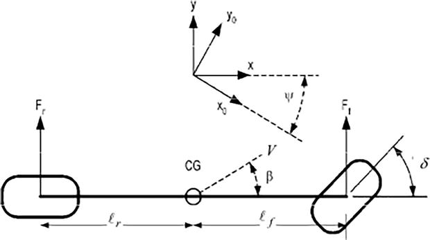
Figure 1.

Diagram of bicycle model [5].

$$\begin{array}{c}\dot{x}=\mathit{\text{vcos}}\left(\psi +\beta \right)\\ \dot{y}=\mathit{\text{vsin}}\left(\psi +\beta \right)\\ \dot{\psi }=\frac{v}{l_r}\mathit{sin}\left(\beta \right)\\ \dot{v}=a\\ \dot{\beta }=\mathit{arctan}\left(\frac{l_r}{l_f+l_r}\mathit{tan}\left({\delta }_f\right)\right)\end{array}$$E3

This model is inherently nonlinear due to the rotation of the front tire as an input and its corresponding impact on the system as a whole. As such, it is sometimes useful to linearize this system about a zero steering angle in order to develop the linearized kinematic bicycle model. This model describes the kinematic motion of a front-steered vehicle well but makes one assumption that greatly limits its performance. The kinematic model’s assumptions imply that the vehicle’s front and rear wheels will drive forward in exactly the direction they are aimed, which is not true, especially at larger steering angles. In reality, tires flex and the contact patch where the tire meets the road can distort, leading to behavior that does not fit this model. At higher lateral accelerations, tire dynamics become one of the most significant parameters in lateral control.

3.2 Dynamic bicycle model

The dynamic model is an expanded form of the kinematic model, in that tire forces are now included. Tire behavior is nonlinear and does saturate beyond a certain threshold. The most famous model used in both academia and industry is the Pacejka Magic Tire formula, which was empirically derived from a series of experiments designed to capture pure cornering motion [6]. Though there is not a direct link to known physical phenomena within the tire, the Magic Formula accurately captures tire behavior over a wide range of conditions.

$$F_y\left({\alpha }_y\right)=D_y\mathit{sin}\left(C_y\mathit{arctan}\left(B_y\ast {\alpha }_y-E_y\left(B_y{\alpha }_y-\mathit{arctan}\left(B_y{\alpha }_y\right)\right)\right)\right)+S_{V_y}\text{where}{\alpha }_y=\alpha +S_{H_{y.}}$$E4

In this model, coefficients A, B, C, D, and E are curve fit to a set of experimental observations, while the S parameters are linear shifts. These parameters remain valid for a vehicle so long as tire load F_z and camber remain constant. For a bicycle model, this does not add any additional assumptions. This model can be directly incorporated as the lateral tire force, or if desired linearized about the origin to produce the more simple relation.

$$F_y=C_y{\alpha }_y$$E5

This assumption simplifies the model but loses the ability to model tire saturation, and therefore, only performs adequately within a near-linear range. Below a lateral acceleration of 4–5 m/s², this model is sufficient for most applications. When incorporated into the linear bicycle model, the state space notation for lateral motion of a bicycle model becomes

$$\left[\begin{array}{c}\dot{v}\\ \dot{r}\end{array}\right]=\left[\begin{array}{cc}-\frac{C_r+C_f}{\mathit{mu}}& -u-\frac{C_f{a}_1-C_r{a}_2}{\mathit{mu}}\\ \frac{-C_f{a}_1+c_r{a}_2}{u{I}_z}& \frac{-C_f{a}_1^2-C_r{a}_2^2}{I_{z}u}\end{array}\right]\left[\begin{array}{c}v\\ r\end{array}\right]+\left[\begin{array}{c}\frac{C_1}{m}\\ \frac{C_f{a}_1}{I_z}\end{array}\right]{\delta }_f$$E6

$$y_e=\left[01\right]\left[\begin{array}{c}v\\ r\end{array}\right].$$

3.3 Additional higher complexity models

Additional higher-order models of note include the planar and double bicycle models, which model each tire with a fixed track width between two linked bicycle models, and the full model, which can consider roll and weight transfer. There are a limitless number of considerations that can be made, but each additional required state exponentially increases the computation time required for an MPC controller to generate the optimal solution, and as of yet are not feasible without a significant investment into the computational platform. The following examples will use more simple models for ease of explanation as well as viability for use without heavy resource commitments.

4. Model predictive control of an autonomous vehicle

In recent years, model predictive control has become of great interest in autonomous vehicle engineering, as it is able to formulate an optimal control law given realistic vehicle constraints, and adjust in real-time to a change in target trajectory as well as vehicle dynamic conditions. It is adaptable to a wide variety of applications and provides a great deal of flexibility to the control designer. However, the greatest limiting factor is the computation time required to achieve an optimal solution. In practical applications, significant time must be given to ensure that the controller will achieve good performance and provide commands quickly enough to function in a real-world environment. A rule of thumb in this application is the outermost loop of the controller should iterate at roughly 10 Hz frequency, which has been used several times in academic studies [7, 8]. Currently, computing technology has advanced to the degree that both linear and nonlinear MPC controllers are beginning to see use. In this section, the MPC formulation of a vehicle controller will be elucidated, and considerations will be noted with regard to realistic functional development (Figure 2).

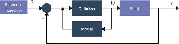
Figure 2.

MPC loop structure.

4.1 MPC general problem—Structure

The general formulation of a model predictive controller in the sense of automotive control is to solve a constrained optimization problem to generate optimal steering and velocity commands, which can reliably follow a reference trajectory. This optimization is performed by minimizing a cost function, which enables the designer to tune the system’s response intuitively by weighing the significance of different states, as well as state transition speeds and a variety of other factors. The general formulation of a continuous-time optimal control problem is as follows:

$$\begin{array}{c}\underset{x,u}{\mathit{minimize}}\int l_c\left(x\left(t\right),u\left(t\right)\right)\mathit{dt}+V_{f}x\left(T\right)\\ \begin{array}{ccc}\text{subject to}:& x\left(0\right)=x_0& \\ & \dot{x}\left(t\right)=f\left(x,u\right)& t\in \left[0,T\right]\\ & \left(x\left(t\right),u\left(t\right)\right)\in \mathbb{Z}& t\in \left[0,T\right]\\ & x\left(T\right)\in {\mathbb{X}}_f& \end{array}\end{array}$$E7

In this formulation, l_c is a cost function of the states and inputs, while V_f is a terminal constraint associated with the final state in the time horizon. This general formulation assumes that the states are defined only as a function of states and inputs, as well as that the states and inputs are bounded in some finite space, as is the terminal state.

This problem in its current state is unwieldy, as in continuous time, there are an infinite set of states x and u in the considered time range to be optimized. There are two main classes of methods, known as direct and indirect methods. While both methods have merits in their own right, direct methods tend to produce a solution more quickly (by sacrificing the guarantee of optimality). The primary difference is that indirect methods will optimize some approximate results in continuous time, then convert this solution to a set of discrete commands, while direct methods discretize the system first before solving the optimization problem. Since speed is critical, this chapter will focus primarily on direct methods. To begin, the system must be discretized to become solvable within a meaningful length of time. Discretization methods vary slightly depending on the choice of optimization variables, but there are a few requirements for all discrete systems used in MPC.

Time step—The most basic component of a discrete system, the continuous system is subdivided by an equal time step. Smaller time steps imply a larger computational cost but also a corresponding increase in resolution of the control output.

Time horizon—MPC employs a receding horizon, that is to say that each iteration of the outer loop minimizes within a fixed time horizon. In simple terms, if the receding horizon is 10 seconds, the algorithm will minimize the cost function for the set of all time steps within the next 10 seconds from the current time. The time horizon should at minimum be selected to be sufficiently long that the controller can project a trajectory that converges to the path where possible, as a shorter horizon time can result in a non-stabilizing controller.

Input assumption—For practical MPC controllers, the input u is considered to be piecewise constant within each time step, sometimes referred to as the step input condition. In some cases, this can be relaxed but for the purposes of this chapter, other conditions will not be considered as they require a different approach to optimization.

4.2 Formulation and transcription

For reasons that will be clear to those with experience using cost functions, and that will be explained later in the section, it is practical and many times ideal to use a quadratic cost function similar to an LQR formulation. In the example below, there is a quadratic cost for the states, inputs, derivative of inputs, and final value.

$$J=x^T\mathit{Qx}+u^T\mathit{Ru}+{\dot{u}}^T{R}_{\Delta }\dot{u}+\Phi \left(x_f\right)$$E8

This cost function is a specific implementation of the general formulation described earlier, in that Q describes a quadratic state cost, R describes a quadratic input cost, R_Δ describes a quadratic cost to a change in input, and ɸ describes a scalar terminal cost. In comparison to the general form, J replaces l_c and V_f in the optimization problem.

Using the assumption that inputs within a time step are piecewise constant, with such a cost function, it is possible to convert the boundary value problem to an initial value problem; that is to say that an optimizer needs to solve for a constant input that minimizes the cost function across its specific time step. This is referred to as a shooting method and has the greatest potential for real-time applications.

4.3 Direct shooting methods

Direct shooting methods are the simplest methods that can be applied to produce a performant output, and exploit the formulation described in previous sections. Since the boundary problem has been converted to an initial value problem, an optimizer can, within each time step, guess and check the input value and observe the output, moving closer to the optimal value with each iteration. The solving method by which this is guaranteed to approach an optimal solution will be described in the next section, as well as the constraints imposed on the initial value optimization method. Once an optimal solution is found, its final state values are used to generate the next initial value problem in the set. This process is repeated until the time horizon is reached.

Direct multiple shooting is an extension of direct single shooting [9]. Instead of solving the first time step, then continuing forward in time to reach a solution, direct multiple shooting methods solve each time step in parallel, allowing a discontinuity between the time steps to appear—this is called a defect. The defect is then included in the optimization problem as a term to be minimized, and thus after iteration becomes negligible. If an optimal solution is reached, the absolute sum of defects should approach zero. Now that the transcription method and optimization problem have been formulated, the only remaining component is how the optimization problem is actually solved.

5. Solving the optimization problem

Direct methods require the use of an iterative solver, which approaches the final result in finite time. In this section, a few selected solver methodologies will be described and compared, starting with a basic solver to describe their fundamental behavior, before moving on to more complex methods. An important clarification is to be made with regard to optimization and its degree of difficulty. While distinction is generally made between linear and nonlinear MPC, the more significant factor determining the difficulty of optimization is whether the system is convex or non-convex. This is the primary reason that quadratic cost functions are preferred, which was referenced earlier in the chapter. Quadratic cost functions maintain convexity in the solution space. Linear MPC with a quadratic cost function will always be a convex optimization problem, while nonlinear MPC may or may not be convex. Convexity in this context assumes that all points between two points in the set are also points in the set. This enables the use of interior point methods to generate a solution, which comprises the driving functions behind most popular optimization solvers used in MPC. Additionally, a convex set provides a guarantee that the solution will be globally optimal [10]. Optimization for non-convex problems introduces the risk that the solution will only be locally optimal, but there are techniques to mitigate this issue without making the computation time unrealistic for use in real-time applications like autonomous vehicle control.

One popular method for optimization is the Newton–Raphson method. This gradient descent method is a simple implementation that provides a good basis for understanding other optimization techniques. The formula for selecting the next iterative point is shown below:

$$x_{k+1}=x_k-{\left({\nabla }^{2}f\left(x_k\right)\right)}^{-1}\nabla f\left(x_k\right).$$E9

This method uses the Hessian of a function to approximate the global minima, as this in a sense minimizes a quadratic cost function. One benefit of this method is that it works very well for linear systems without a large number of states, with low relative computational cost. However, significant nonlinear behavior or a large number of states may require more advanced methods. Optimization is a large field with a wide breadth of literature so will not be covered in depth here, but the Newton–Raphson method provides a good intuitive sense of the general idea of how optimization is performed in a model predictive controller.

6. Simulations

In order to provide a more concrete and understandable model, two MPC simulations were selected to present their performance. There will not be a one-to-one comparison as each controller has a different application, but a curious reader will be able to use the available GitHub repositories to investigate beyond the phenomena and commentary provided here.

6.1 Linear MPC

A simple example of linear MPC using a kinematic bicycle model is available at the PythonRobotics GitHub repository [11]. The available model predictive speed and steering control utilizes a cubic spline planner to produce a set of ordered waypoints, which include an x, y, and yaw pose as well as velocity target. The simulation uses the direct single-shooting method based on the same cost function described earlier in this chapter. The map used in this example is derived from the nonlinear example presented next in this section (Figure 3).

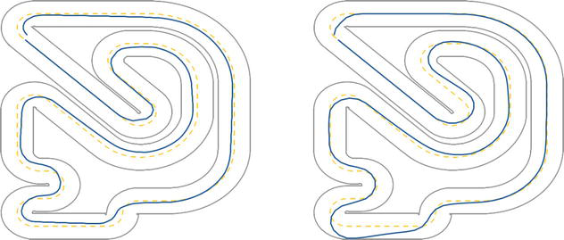
Figure 3.

PythonRobotics linear kinematic model (5 m/s and 10 m/s, respectively).

In this example, the MPC controller was modified to have a fixed longitudinal velocity, in order to accentuate the lateral behavior of the vehicle. In this linear example, which was simulated with a kinematic system, the vehicle is able to track the target path, however, performance is hindered at higher speeds. The most significant overshoot is observed in the lower left section of the track, where the linear model is unable to generate an ideal trajectory for a high curvature. Additionally, this model is able to effectively control for cross-track error and yaw rate but is limited in practical scope as it cannot make use of additional road information.

A much more advanced example from ETH Zurich presents a nonlinear model predictive control scheme, which incorporates a set of realistic constraints to the vehicle and path, and simulates a higher-order model, a dynamic bicycle model with Pacejka tire coefficients [12]. Again, this simulation was restricted to only allow for lateral control and was operated at a fixed speed of 5 and 10 meters per second. However, this example has a more developed cost function, and as such select weights are compared to differentiate between a forward-progression optimization and path-tracking optimization.

$$\begin{array}{c}J=e_c^T{q}_c{e}_c+e_l^T{q}_l{e}_l+\Delta u^T{R}_{\Delta }\mathit{\Delta u}\\ \begin{array}{ccc}\text{Subject to}:& x\left(0\right)=x_0& \\ & \dot{x}\left(t\right)=f\left(x,u\right)& \\ & e_l\left(x\right)=\mathit{sin}\left({\varphi }_{\mathit{ref}}\right)\left(X-X_{\mathit{ref}}\right)-\mathit{cos}\left({\varphi }_{\mathit{ref}}\right)\left(Y-Y_{\mathit{ref}}\right)& \\ & e_c\left(x\right)=-\mathit{cos}\left({\varphi }_{\mathit{ref}}\right)\left(X-X_{\mathit{ref}}\right)-\mathit{sin}\left({\varphi }_{\mathit{ref}}\right)\left(Y-Y_{\mathit{ref}}\right)& \\ & x\in {\mathbb{X}}_{\mathit{\text{track}}}& \end{array}\end{array}$$E10

This formulation is still quadratic but uses a lag cost term q_c as well as state, input, and terminal cost. The state costs are also bounded within a track, which constrains the optimization such that the vehicle cannot predict a path that leaves the track (Figure 4).

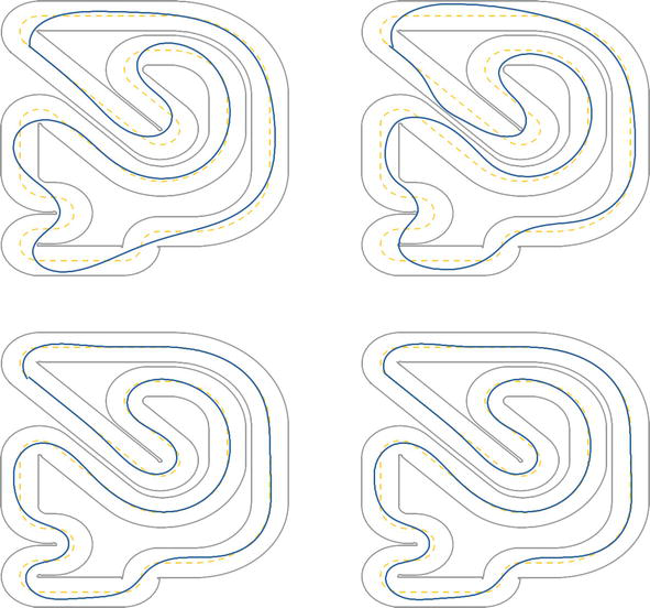
Figure 4.

Modified MPCC controller simulation at select speeds and optimization weights.

Tracking optimization is performed by increasing relative weight to both of the error states e_l and e_c, while progression optimization is made by increasing the relative weight of the lag cost parameter e_l included in this cost function. This presents a functional means to tailor the cost function to the specific vehicle application. For an average passenger vehicle, the performance of the tracking optimized cost functions would serve as more useful while a race car would benefit from the increased emphasis on forward progress over strict path tracking. Additionally, the nonlinear model is able to benefit from the characteristics of the tire to achieve very precise motion around the tight lower left bend, while avoiding collision with the side of the road due to the constraints placed on the controller. The PythonRobotics method, using single shooting without an optimization library, has a controller frequency of about 10 Hz, while the MPCC (model predictive contouring control) method was able to provide commands at nearly 200 Hz on the same platform. This is due to the implementation of multiple shooting as well as the inclusion of a performance-based optimization library.

7. Conclusions

The comparison presented in this chapter illustrates the importance of implementation when designing an MPC controller. Though the PythonRobotics model is simpler and possesses fewer states, it runs significantly slower than the MPCC controller. This is primarily due to two key factors—coding language and optimization style. Direct multiple shooting converges faster than single shooting due to the increased dimensionality of slack parameters between each time step. Furthermore, Python is inherently a slower language than C++ because is it not a compiled language. In the application of autonomous vehicles, where fast control response is essential, it is of the utmost importance to formulate the problem and design using languages that reduce the computational time wherever possible.

The benefits of model predictive control are additionally shown in the simulated examples above, especially the MPCC controller, which utilizes bounded optimization to navigate the track near the edge of the drivable terrain. Without an intelligent path planner, it is difficult to design a controller through any other means that is able to use information about the drivable space and optimize the control response to take advantage of it. While this effect is achievable with more complex path planning and replanning, model predictive control is able to provide a collision-free output whose performance is dependent upon the model itself rather than an external planning algorithm. More advanced autonomous systems are additionally able to forward-project moving objects, and a model predictive controller can take these projections and generate an online output that navigates around such objects.

In existing real-world applications, longitudinal control is additionally incorporated in order to have the vehicle achieve a form of full-optimized piloting. This provides a significant advantage in some cases as many other controllers require either a decoupling of the longitudinal and lateral control or some modification to the control law to achieve good performance. The increased computational cost of this controller is quickly becoming a smaller and smaller price to pay for this performance, and the nonlinear model predictive control of a passenger vehicle is becoming increasingly feasible to implement. Collision avoidance, behavioral prediction models, and stochastic prediction are just a few of the many possible improvements that can be incorporated to achieve control with a well-defined set of safety considerations. This will ultimately provide an extra layer of safety and performance in the computational stack of a self-driving vehicle, beyond just following a dictated path.

Code GitHub Repositories

https://github.com/AtsushiSakai/PythonRobotics

https://github.com/alexliniger/MPCC

References

- 1.
Hoffmann GM et al. Autonomous automobile trajectory tracking for off-road driving: Controller design, experimental validation and racing. In: American Control Conference, New York, NY. 2007. DOI: 10.1109/acc.2007.4282788 - 2.
Assadian F, Mallon KR. Robust Control: Youla Parameterization Approach. Hoboken, New Jersey: John Wiley & Sons Ltd; 2022 - 3.
Rafaila RC, Livint G. H-Infinity Control of Automatic Vehicle Steering. In: 2016 International Conference and Exposition on Electrical and Power Engineering (EPE), Iaşi, Romania. 2016. DOI: 10.1109/icepe.2016.7781297 - 4.
Khalil HK. Nonlinear Systems. 3rd Edition. Upper Saddle River: Prentice Hall; 2002 - 5.
Rajamani R. Vehicle Dynamics and Control. 2nd Edition. Berlin: Springer; 2012. DOI: 10.1007/978-1-4614-1433-9 - 6.
Pacejka HB, Bert CW. Tyre models for vehicle dynamics analysis. Journal of Applied Mechanics. 1995; 62 (1):268-268. DOI: 10.1115/1.2895925 - 7.
Zeng J et al. Safety-Critical Model Predictive Control with Discrete-Time Control Barrier Function. In: American Control Conference (ACC), New Orleans, LA. 2021. DOI: 10.23919/acc50511.2021.9483029 - 8.
A Predictive Path-Following Controller for Multi-Steered Articulated ... https://arxiv.org/pdf/1912.06259v4 - 9.
Bock HG, Plitt KJ. A multiple shooting algorithm for direct solution of optimal control problems *. IFAC Proceedings Volumes. 1984; 17 (2):1603-1608. DOI: 10.1016/s1474-6670(17)61205-9 - 10.
Schwenzer M et al. Review on model predictive control: An engineering perspective. The International Journal of Advanced Manufacturing Technology. 2021; 117 (5–6):1327-1349. DOI: 10.1007/s00170-021-07682-3 - 11.
Sakai A et al. PythonRobotics: A Python Code Collection of Robotics Algorithms - 12.
Liniger A et al. Optimization-Based Autonomous Racing of 1:43 Scale RC Cars. Optimal Control Applications and Methods. 2014; 36 (5):628-647. DOI: 10.1002/oca.2123