Stereo-Measurement of 3D Poses of a Walking Person with a Puppet Model and Low-Rank Filter

Abstract

In order to achieve safety and security in public places by recognizing people’s behavior, we have to measure a person’s pose and capture his or her movement. Conventionally, it was hard to recognize the person itself before capturing the pose, and research has been carried out based on the silhouette of the person obtained by performing such as background subtraction. Efficient recognition was difficult in using silhouettes because they were greatly affected by the observation direction. Since the difficulty disappears if we adopt three-dimensional processing, some methods using Kinect have been proposed. Unfortunately, their performance was limited in the usage environment. Here OpenPose is applied to the stereo-pair images for getting the two-dimensional coordinates of the joint points. The coordinates may fluctuate depending on the lighting. Assuming the fluctuation follows a Gaussian distribution, the three-dimensional coordinates will be mixed with a larger noise component following a Cauchy distribution. Since the Cauchy distribution does not have a defined mean and variance, we can not achieve the desired smoothing even with averaging. The method described here provides stable poses that can withstand subsequent use by applying a low-rank filter and a puppet model in which the distance between joint points is invariant.

1. Introduction

Recognizing the behaviors of people in public spaces such as train stations is very important to ensure our safety and security. For example, even if a person feels sick, falls, or has trouble with another person while walking, we can automatically recognize it and can help the person immediately. A person’s behavior can be defined as a time trace pattern of poses of the person. In other words, if the pose can be quantified, it is possible to recognize the behavior as a pattern of temporal change. For the quantification, it is first essential to be able to measure the pose with high precision. There have been many methods for recognizing human poses [1, 2, 3]. They can be divided into two groups: silhouette-based methods and joint-based ones. In the former group, human silhouettes were obtained, for example, by a background subtraction or by calculating optical flow [4], and were used to analyze the behavior. In the latter, joint positions measured by Kinect were used [5, 6, 7, 8]. The silhouette-based methods, however, had difficulties in estimating the poses. It was not easy to find some feature points to describe the pose from the silhouette. On the other hand, the joint-based methods easily described the pose as the placing of the joint points. In particular, Kinect gave us three-dimensional positions of them and made the analysis easier. Unfortunately, Kinect projected a dot pattern to obtain the distance to a target, so there were some problems such as limitations in measurable distance and outdoor environment. OpenPose [9] was also one of the solutions. It gave us 25 keypoints, including human joints on an image. The two-dimensional coordinates were useful in describing poses in a walk perpendicularly crossing the optical axis [10]. The OpenPose-based method had similar problems to the silhouette-based one. The size change of the pose with the distance made the analysis more complicated. Some solutions have been required.

In this paper, we propose a measurement method for obtaining three-dimensional joint coordinates of a human pose by applying OpenPose to a sequence of stereo-pair images. We obtain the three-dimensional joint coordinates from the two-dimensional coordinate pair of the same joint extracted by OpenPose in each of the stereo-pair images. This means that we quantify the pose of a person in the three-dimensional space with a small number of joints. Recently, OpenPose provided the three-dimensional keypoint features with a demo. It, however, requires a specific multi-camera system and has some barriers to use for general motion measurements. Here we construct a software system for obtaining three-dimensional joint coordinates using a single general-purpose stereo camera. The stereo-measurement also has the feature of being able to acquire a person’s pose from a distance. Therefore, we can measure the poses of multiple persons simultaneously in a wide area. The joint coordinates reconstructed from stereo-pair two-dimensional ones are severely affected by missing values and/or some fluctuations contained in OpenPose output. Therefore, noise reduction is essential in the proposed method. When we obtain the three-dimensional coordinates, a parallax on stereo-pair images is included in the denominator of the stereo-vision formula. Therefore, Gaussian fluctuation in the stereo-pair images appears as a larger noise component following a Cauchy distribution on the three-dimensional coordinates. Since the mean and the variance of the Cauchy distribution are undefined, simple averaging against Gaussian noise does not achieve an expected smoothing. We need another approach for the noise reduction in the three-dimensional coordinates. We regard walking as being consisted of a kind of periodical movement with a spatial correlation structure among all joints. Therefore, we focus on the dominant mode of them as the signal component to be measured. We realize the noise reduction by extracting the low-rank component [11] of the time sequence of joint coordinates recognized by OpenPose. We call It a low-rank filter (LRF). Applying LRF separately to each joint data may destroy the spatial structure. Therefore, we compensate the joint coordinates using a puppet model [12] introduced from the fact that every bone length, that is distance between two joints, is invariant for any pose. Severe noise included in measured coordinates of the joints yields many candidates of the pose to be obtained. Those poses include meaningless ones as the human posture. The puppet model enables us to eliminate the meaningless poses by fixing the length of the upper and lower limbs without restricting the angle between the limbs. The length fixing acts as some kind of constraint. Thus, knowledge about the object makes meaningful measurement and recognition even in adverse conditions. In the following sections, we describe the principle and the procedure of the method. Application results of an actual person walking are also shown.

2. Principle

In order to realize direction-free analysis for human walking, we consider a remotely joint-based measurement using stereo-vision. In the conversion from the joint coordinates in both stereo-pair images to three-dimensional ones, Gaussian noise expands to a terrible one following the Cauchy distribution. Therefore, the main task of this research is to reduce the severe noise and to get accurate three-dimensional joint coordinates. We consider that human joints do not move randomly but move with a mutual spatial correlation structure. From this fact, we introduce a puppet model that acts to restrict the joint position in an area.

2.1 World and camera coordinate system

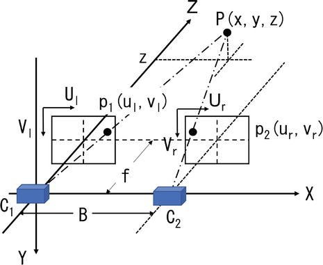
Figure 1 shows world and camera coordinate systems used here. A set of stereo-camera $C_1$ and $C_2$ are calibrated (distortion correction and collimation are performed) so that their optical axes are parallel and have the same focal length with distance $B$. They are installed so that the center of the camera $C_1$ coincides with the origin of the world coordinate system.

Figure 1.

World and camera coordinate systems.

A point $P\left(x,y,z\right)$ on the world coordinate system is observed as image points $p_1\left(u_l,v_l\right)$ and $p_2\left(u_r.v_r\right)$ on cameras $C_1$ and $C_2$, respectively. The coordinates $x,y,z$ are obtained as

$$x=\frac{u_{l}B}{u_l-u_r},y=\frac{v_{l}B}{u_l-u_r},z=\frac{\mathit{fB}}{u_l-u_r},$$E1

where, $f$ is the focal length and $B$ baseline length. The camera coordinates $u_l,v_l$ and $u_r,v_r$ are also calculated from the coordinates $x,y,z$ as

$$u_l=f\frac{x}{z},u_r=f\frac{x-B}{z},v_l=v_r=f\frac{y}{z}.$$E2

Gaussian noise contained in joint coordinates $u_l$, $v_l$, $u_r$_, and $v_r$ observed on both stereo-pair images appear in each of the numerator and the denominator of Eq.(1). Since the ratio of two random normal distributed variables with mean 0 and different variances follows the Cauchy distribution [13], obtained three-dimensional joint coordinates $x$, $y$, and $z$ are severely affected by noise following a Cauchy distribution. The first and second moments of the Cauchy distribution diverge to infinity, its mean and variance are not defined. This means a simple averaging does not achieve the expected smoothing.

2.2 OpenPose and keypoint coordinates

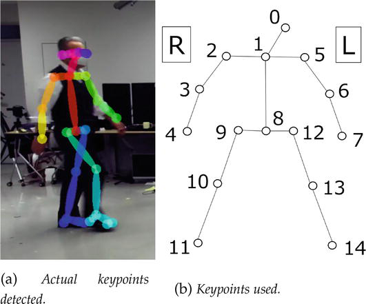
OpenPose is the first real-time multi-person system to jointly detect human body, hand, facial, and foot keypoints [9]. Here we use it as a human joint detector and adopt 15 keypoints for human walking analysis among the output format BODY_25, as shown in Figure 2. OpenPose provides the keypoint with detection confidence in a JSON file. The confidence takes a value between 0 and 1, and the higher the value the more confident it is. When a joint is hidden by the body, its confidence takes 0, and the coordinates are also 0. Therefore, the missing coordinates such as due to joint occlusion yield larger noise. We have to complete the missing values first. OpenPose may also cause incorrect detections, such as leg swapping, arm swapping, leg duplication, and arm duplication, due to poor lighting conditions in image capturing. In those cases, the confidence takes lower but non-zero values, so it is hard to detect them using confidence. Both the swapping and the duplication also cause larger noise, so we need some algorithms to detect and correct them.

Figure 2.

OpenPose keypoints in BODY_25.

2.2.1 Missing value interpolation

Our strategy for interpolating the missing values is to fill them in a simple way, then smooth them with preserving features. Let $\left\{s_1,\dots ,s_i,\dots ,s_j,\dots ,s_n\right\}$ be a sequence of measured coordinates with some missing values as

$$s_k\left\{\begin{array}{ll}=0& \left(i\le k\le j\right)\\ \ne 0& \left(\mathit{\text{others}}\right)\end{array}\right..$$E3

Those missing values are interpolated by using internal division points of both ends of non-zero-confidence observations as

$$s_k=\frac{s_{i-1}\left(j-k+1\right)+s_{j+1}\left(k-i+1\right)}{j-i+2}\left(i\le k\le j\right).$$E4

When $j=n$, we use $s_k=s_{i-1}\left(i\le k\le n\right)$, and $i=1$ we use $s_k=s_{j+1}\left(1\le k\le j\right)$.

2.2.2 Keypoint swapping and duplication

In wrong recognitions, left and right legs are duplicated as one leg, and leg swapping also occurs more frequently. In normal walking, one of the legs is swung to the front and fixed on the floor, and the other is also swung and fixed alternately. The left and right ankles draw continuous trajectories that accurately reflect these movements. When the leg swapping and/or duplication occur, some discontinuities are yielded in the trajectories. Therefore, we detect them by finding the discontinuities. We detect the swapping by finding the discontinuity at the same position on both left and right ankle trajectories, and the duplication by finding it on one of them. For simplicity, consider a person walking parallel to the x-axis as shown in Figure 2. Let x-coordinate vectors of left and right ankles be ${\mathit{s}}_L={\left(s_{L1}{s}_{L2}\dots s_{\mathit{Ln}}\right)}^T$ and ${\mathit{s}}_R={\left(s_{R1}{s}_{R2}\dots s_{\mathit{Rn}}\right)}^T$ for $n$ observations. Their elements $s_{\mathit{Li}}$ and $s_{\mathit{Ri}}\left(i=1,\dots ,n\right)$ are relative position to a keypoint mid-hip. The swapping is detected at the i-th element when ${\delta }_{\mathit{Li}}/w>\mathit{\text{threshold}}$ and ${\delta }_{\mathit{Ri}}/w>\mathit{\text{threshold}}$, where, $w$ means the stride length of the walk as

$$w=min\left(max\left({\mathit{s}}_L\right)-min\left({\mathit{s}}_L\right),max\left({\mathit{s}}_R\right)-min\left({\mathit{s}}_R\right)\right),$$E5

$${\delta }_{\mathit{Li}}=\mid s_{\mathit{Li}}-s_{\mathit{Li}-1}\mid ,$$E6

$${\delta }_{\mathit{Ri}}=\mid s_{\mathit{Ri}}-s_{\mathit{Ri}-1}\mid .$$E7

2.2.3 Vertical averaging

As already mentioned, stereo-cameras are also parallelized by the calibration. Therefore, there should be no difference in vertical coordinates between corresponding joints on the stereo-pair images. If the difference exists, it is considered to be due to noise, and we replace those vertical coordinates with their average values. Thus, OpenPose joint data are completed.

2.3 Pose vector and behavior matrix

In this study, we define behavior as the temporal change of the poses. Therefore, it is necessary to quantify each pose for describing the behavior. We define keypoint vector ${\mathit{q}}_{\mathit{t}}$ and the pose vector ${\mathit{p}}_{\mathit{t}}$ independently of the dimension. The former is described as

$${\mathit{q}}_t=\left(u_0^t{v}_0^t{u}_1^t{v}_1^t\cdots u_{m-1}^t{v}_{m-1}^t\right),$$E8

on an image or

$${\mathit{q}}_t=\left(\begin{array}{cccccccccc}{x}_0^t& y_0^t& z_0^t& x_1^t& y_1^t& z_1^t& \cdots & x_{m-1}^t& y_{m-1}^t& z_{m-1}^t\end{array}\right),$$E9

in the world coordinate system, where, $\left(u_i,v_i\right)$ and $\left(x_i,y_i,z_i\right)\left(i=0,\cdots ,m-1\right)$ are two- and three-dimensional coordinates of the keypoints, respectively, and $m=15$. Of course, since the 2D pose strongly depends on the direction of observation, the 3D pose vector without such dependence is valid. Therefore, when we simply refer to the pose vector, we mean the 3-D one. Using their relative coordinates, the latter is represented as

$${\mathit{p}}_t=\left(\begin{array}{cccccc}{u}_0^t-u_8^t& v_0^t-v_8^t& \cdots & \cdots & u_{m-1}^t-u_8^t& v_{m-1}^t-v_8^t\end{array}\right),$$E10

on an image or

$${\mathit{p}}_t=\left(\begin{array}{ccccccc}{x}_0^t-x_8^t& y_0^t-y_8^t& z_0^t-z_8^t& \cdots & x_{m-1}^t-x_8^t& y_{m-1}^t-y_8^t& z_{m-1}^t-z_8^t\end{array}\right),$$E11

in the world coordinate system, where, $\left(u_8,v_8\right)$ and $\left(x_8,y_8,z_8\right)$ are coordinates of the keypoint mid-hip at time $t$, and ${\mathit{p}}_t$ does not include it while ${\mathit{q}}_t$ does. We consider that the keypoint mid-hip is located near the true centroid of a human body, so we use it instead of the centroid. Thus, the pose vector is useful to represent relative pose regardless of the position. Finally, we define keypoint matrix $Q_n$ and behavior matrix $P_n$ for $n$ observations as

$$Q_n=\left(\begin{array}{c}{\mathit{p}}_0\\ {\mathit{p}}_1\\ ⋮\\ {\mathit{p}}_{n-1}\end{array}\right),P_n=\left(\begin{array}{c}{\mathit{p}}_0-\mathit{\mu }\\ {\mathit{p}}_1-\mathit{\mu }\\ ⋮\\ {\mathit{p}}_{n-1}-\mathit{\mu }\end{array}\right),\mathit{\mu }=\frac{1}{n}\sum _{i=0}^{n-1}{\mathit{p}}_i.$$E12

The covariance matrix of the behavior matrix is also obtained as

$$\mathrm{\Sigma }=\frac{1}{n-1}{P}_n^T{P}_n.$$E13

Since the elements within the covariance matrix represent the degree of correlation between corresponding coordinates, we consider that it includes important information about the spatial correlation structure of joint movements.

2.4 Auto-regression model and low-rank filter

OpenPose may yield some fluctuations in its recognitions, and pose vectors still have noise due to the fluctuation. Since they severely affect the three-dimensional coordinates, we have to reduce the noise in the pose vectors. On the other hand, the coordinates have some correlation structures, such that they do not change abruptly in time while keeping their relative positions. Therefore, we realize the noise reduction by extracting low-rank components from the observed time sequential joint coordinates. The one-dimensional coordinate sequence is once converted to a two-dimensional matrix shape to extract the low-rank components. After we apply a rank reduction operation to that matrix, the resultant matrix is converted back to the original one-dimensional sequence. To perform the process, we need an interconversion algorithm between a one-dimensional signal and a two-dimensional matrix. Let ${\mathit{U}}_k$ be a temporal observation vector of positions of the k-th joint of a moving person on the image as

$${\mathit{U}}_k=\left(\begin{array}{cccc}{u}_k^0& u_k^1& \cdots & u_k^n\end{array}\right),$$E14

where, the superscripts show time, that is, frame. Since the movement is not so fast and not random, they have some correlation with each other. This means that they fit into an auto-regressive (AR) model with length of $m$ as

$$\left\{\begin{array}{l}{u}_k^m=a_0{u}_k^0+a_1{u}_k^1+\cdots +a_{m-1}{u}_k^{m-1}\\ u_k^{m+1}=a_0{u}_k^1+a_1{u}_k^2+\cdots +a_{m-1}{u}_k^m\\ ⋮\\ u_k^n=a_0{u}_k^{n-m}+a_1{u}_k^{n-m+1}+\cdots +a_{m-1}{u}_k^{n-1}\end{array}\right..$$E15

These equations show that the current value of a one-dimensional signal is determined by the values of the $m$ signals preceding it. Using matrix format, we rewrite Eq. (15) as

$$\left(\begin{array}{cccc}{u}_k^0& u_k^1& \cdots & u_k^{m-1}\\ u_k^1& u_k^2& \cdots & u_k^m\\ ⋮& ⋮& \ddots & ⋮\\ u_k^{n-m}& u_k^{n-m+1}& \cdots & u_k^{n-1}\end{array}\right)\left(\begin{array}{c}{a}_0\\ a_1\\ ⋮\\ a_{m-1}\end{array}\right)=\left(\begin{array}{c}{u}_k^m\\ u_k^{m+1}\\ ⋮\\ u_k^n\end{array}\right),$$E16

and for short as

$$X\mathit{A}=\mathit{Y},$$E17

where matrix $X$ is called the Hankel matrix. The vector $\mathit{Y}$ is calculated from the matrix $X$, and also $X$ is reconstructed from $\mathit{Y}$. Considering that the observations consist of dominant signal component with some correlation structure and some noise, Eq. (17) can be described as

$$\left(X_s+X_n\right)\mathit{A}=\left({\mathit{Y}}_s+{\mathit{Y}}_n\right).$$E18

Here we realize the low-rank filter for the vector ${\mathit{Y}}_s$ by separating $X_s$ with rank $r$ from $X_n$ as

$$X_s{\mathit{A}}_s={\mathit{Y}}_s{\left({\mathit{\text{rankX}}}_s=r_f\right)}_{.}$$E19

Since the coefficient vector $\mathit{A}$ in Eq. (19) is different from that in Eq. (17), an iterative algorithm is needed for the calculation [11].

2.5 Spatial AR model and filtering

As we have already defined, human behavior is a multi-temporal set of poses. We have focused on the temporal correlation structure of each joint in human behavior, and constructed the low-rank filter. Here as an analogy from temporal correlation to spatial one, we propose a spatial AR model. The model is based on the fact that we can estimate the pose of the whole body even if some joints are hidden and cannot be observed. We consider that the linear form of the matrix $X$ in Eq. (17) and its reproducibility from the coordinate vector $\mathit{Y}$ are essential in the low-rank filtering. Therefore, we introduce a matrix and a coordinate vector in the same manner. Let ${\mathit{x}}_j^t$ be the j-th joint coordinates at time t, $\mathbf{0}$ zero coordinates, and ${\mathit{a}}_{\mathit{k}}$ the k-th coefficient vector as

$${\mathit{x}}_j^t=\left(\begin{array}{lll}{x}_j^t& y_j^t& z_j^t\end{array}\right),\mathbf{0}=\left(\begin{array}{ccc}0& 0& 0\end{array}\right),{\mathit{a}}_k=\left(\begin{array}{ccc}{a}_k^x& a_k^y& a_k^z\end{array}\right).$$E20

By analogy to the description of Eq.(16), we propose a new linear matrix equation as

$$\left(\begin{array}{cccc}\mathbf{0}& {\mathit{x}}_1^{t-2}& \cdots & {\mathit{x}}_{m-1}^{t-2}\\ {\mathit{x}}_0^{t-2}& \mathbf{0}& \cdots & {\mathit{x}}_{m-1}^{t-2}\\ ⋮& ⋮& \ddots & ⋮\\ {\mathit{x}}_0^{t-2}& {\mathit{x}}_1^{t-2}& \cdots & \mathbf{0}\\ \mathbf{0}& {\mathit{x}}_1^{t-1}& \cdots & {\mathit{x}}_{m-1}^{t-1}\\ {\mathit{x}}_0^{t-1}& \mathbf{0}& \cdots & {\mathit{x}}_{m-1}^{t-1}\\ ⋮& ⋮& \ddots & ⋮\\ {\mathit{x}}_0^{t-1}& {\mathit{x}}_1^{t-1}& \cdots & \mathbf{0}\\ \mathbf{0}& {\mathit{x}}_1^t& \cdots & {\mathit{x}}_{m-1}^t\\ {\mathit{x}}_0^t& \mathbf{0}& \cdots & {\mathit{x}}_{m-1}^t\\ ⋮& ⋮& \ddots & ⋮\\ {\mathit{x}}_0^t& {\mathit{x}}_1^t& \cdots & \mathbf{0}\end{array}\right)\left(\begin{array}{c}{\mathit{a}}_0\\ {\mathit{a}}_1\\ ⋮\\ {\mathit{a}}_{3m-1}\end{array}\right)=\left(\begin{array}{c}{\mathit{x}}_0^{t-2}\\ ⋮\\ {\mathit{x}}_{m-1}^{t-2}\\ {\mathit{x}}_0^{t-1}\\ ⋮\\ {\mathit{x}}_{m-1}^{t-1}\\ {\mathit{x}}_0^t\\ ⋮\\ {\mathit{x}}_{m-1}^t\end{array}\right).$$E21

The model is characterized by symmetrical calculation such that each joint coordinates x, y, and z on the right side are obtained from all non-zero coordinates on the left side. We believe the symmetrical calculation enables us to realize stable analysis independently of the walking direction. Since the number of unknowns increases threefold, we need at least sequential three poses for the calculation. We use more poses to get the smoothing effect. The filtering is achieved by decreasing the rank of the left-side matrix.

2.6 Puppet models

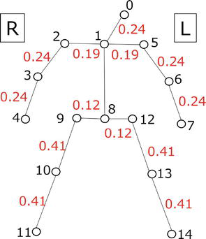
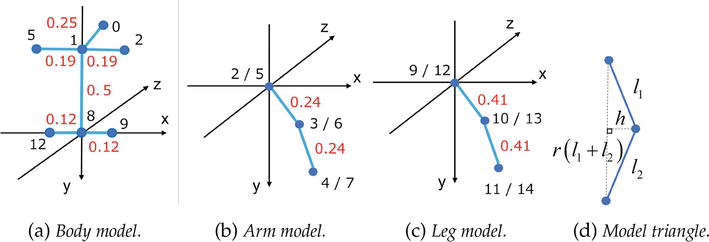
Eq. (1) tells us that fluctuations in observed two-dimensional coordinates ${\mathit{u}}_l$ and ${\mathit{u}}_r$ are expanded and yield severe noise in the three-dimensional ones. Since the noise reduction by using the low-rank filter above is independently applied to each joint observation, it is not enough to reconstruct the meaningful three-dimensional pose. Some constraints are required. Here we propose two types of puppet models as pose stabilizers. The model is based on the fact that the distance between the neighboring joints is invariant of the pose. Figure 3 shows the puppet with the joint number (black) and limb length in [m] (red). The puppet has a symmetrical structure with a predetermined length limb and freely moving joints in any direction. We determined their lengths based on roughly measuring the length of the limbs of a person with a height of 1.7 [m]. We introduce two types of models with different constraint methods: the flexible type and the rigid one. We call the former Puppet-I [12] and the latter Puppet-II. In both models, we regard the keypoint 8 (mid-hip) as the reference joint.

Figure 3.

Puppet model with joint number (black) and limb lengths (red) [m].

2.6.1 Puppet-I

In this model, we evaluate the limb length between a neighboring joint pair whose positions are calculated by using Eq. (1). If the length does not match that of the model, we regard that there is an error in the position of the joint $u_r$ on the right camera image, and adjust the parallax $u_l-u_r$ so that they match. This process is started from the reference joint. Let the position of the i-th neighboring joint $P_i\left(x_i,y_i,z_i\right)$ be calculated from the stereo-pair image points $Q_i^l\left(u_i^l,v_i^l\right)$ and $Q_i^r\left(u_i^r,v_i^r\right)$, and $P_k\left(x_k,y_k,z_k\right)$ be the reference. The parallax adjustment is performed as

$$\mathrm{\Delta }{u}_{\mathit{opt}}^r\leftarrow \underset{\mathrm{\Delta }{u}^r}{argmin}\mid \sqrt{{\left(x_i-x_k\right)}^2+{\left(y_i-y_k\right)}^2+{\left(z_i-z_k\right)}^2}-L_{\mathit{ik}}\mid ,$$E22

where,

$$x_i=\frac{{\mathit{Bu}}_i^l}{u_i^l-u_i^r+\mathrm{\Delta }{u}^r},$$E23

$$y_i=\frac{{\mathit{Bv}}_i^l}{u_i^l-u_i^r+\mathrm{\Delta }{u}^r},$$E24

$$z_i=\frac{\mathit{Bf}}{u_i^l-u_i^r+\mathrm{\Delta }{u}^r},$$E25

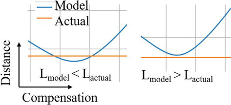
and $L_{\mathit{ik}}$ is the predetermined distance from the reference to the i-th joint. The adjustment is repeatedly applied to successive joint pairs, such as mid-hip to hip, hip to knee, and knee to ankle for legs, and mid-hip to neck, neck to shoulder, shoulder to elbow, and elbow to wrist for arms. The optimization process in Eq. (22) is similar to the finding solution for a quadratic-like curve as shown in Figure 4. Figure 4 indicates that we may have two solutions (left) and have nothing (right). In the former case, we select the best combination so that, for example, both shoulders have the longest distance. Arms and legs are also compensated so that they have the largest angle at the elbow and knee, respectively. In the latter case, the compensation is performed so that the difference becomes the minimum. Substituting the optimal adjuster $\mathrm{\Delta }{u}_{\mathit{opt}}^r$ for the i-th joint into Eqs. (23)–(25), we obtain the three-dimensional coordinate of the joints.

Figure 4.

Model limb length and solutions.

2.6.2 Puppet-II

In this model, we regard that relative positions among body joints, that is, mid hip, left hip, right hip, neck, left shoulder, and right shoulder, are fixed independently of poses. Assuming the rotation angles $\alpha$, $\beta$, $\gamma$ and the shift $x_s$, $y_s$, $z_s$, we transfer the model shown in Figure 5a into the world coordinate system. Then, we predict the position of their joints in both camera coordinate systems. We regard that the measurement was made when the squared sum of the difference among predicted positions $\left(u_l^p,v_l^p\right),\left(u_r^p,v_r^p\right)$ and observed ones $\left(u_l^o,v_l^o\right),\left(u_r^o,v_r^o\right)$ on the camera coordinates for six joints within the part body falls to the minimum and that we obtain the optimum angles and shifts as.

Figure 5.

Rigid body model, upper limb model, and lower one with limb lengths.

$${\mathbf{E}}_{\mathit{opt}}^{\mathit{\text{body}}}\leftarrow \underset{\alpha ,\beta ,\gamma ,x_s,y_s,z_s}{argmin}\sum _{j\in \mathit{\text{body}}}\left\{{\left(u_{l,j}^o-u_{l,j}^p\right)}^2+{\left(v_{l,j}^o-v_{l,j}^p\right)}^2+{\left(u_{r,j}^o-u_{r,j}^p\right)}^2+{\left(v_{r,j}^o-v_{r,j}^p\right)}^2\right\},$$E26

where, ${\mathbf{E}}_{\mathit{opt}}^{\mathit{\text{body}}}$ is the optimized angles and shifts as

$${\mathbf{E}}_{\mathit{opt}}^{\mathit{\text{body}}}=\left(\begin{array}{cccccc}{\alpha }_{\mathit{opt}}& {\beta }_{\mathit{opt}}& {\gamma }_{\mathit{opt}}& x_{\mathit{opt}}& y_{\mathit{opt}}& z_{\mathit{opt}}\end{array}\right),$$E27

and the summation means sum over six joints in the body model (nose is not used), and camera image coordinates are calculated from the initial position of body joints $\left(x_j^{\mathit{\text{init}}},y_j^{\mathit{\text{init}}},z_j^{\mathit{\text{init}}}\right)\left(j\in \mathit{\text{body}}\right)$ as

$$\left(\begin{array}{c}{x}_j^p\\ y_j^p\\ z_j^p\end{array}\right)=R\left(\alpha ,\beta ,\gamma \right)\left(\begin{array}{c}{x}_j^{\mathit{\text{init}}}\\ y_j^{\mathit{\text{init}}}\\ z_j^{\mathit{\text{init}}}\end{array}\right)+\left(\begin{array}{c}{x}_s\\ y_s\\ z_s\end{array}\right)\left(j\in \mathit{\text{body}}\right),$$E28

$$R\left(\alpha ,\beta ,\gamma \right)=\left(\begin{array}{ccc}1& 0& 0\\ 0& \cos \mathit{\alpha }& -sin\alpha \\ 0& \sin \alpha & \cos \alpha \end{array}\right)\left(\begin{array}{ccc}\cos \beta & 0& -sin\beta \\ 0& 1& 0\\ -sin\beta & 0& \cos \beta \end{array}\right)\left(\begin{array}{ccc}\cos \gamma & -sin\gamma & 0\\ sin\gamma & \cos \gamma & 0\\ 0& 0& 1\end{array}\right),$$E29

$$u_{l,j}^p=f\frac{x_j^p}{z_j^p},u_{r,j}^p=f\frac{\left(x_j^p-B\right)}{z_j^p},v_{l,j}^p=v_{r,j}^p=f\frac{y_j^p}{z_j^p}.$$E30

The three-dimensional coordinates of joints in the body are obtained by substituting the optimum angles and shifts into Eq. (28). After body joints measurement, those in the arms and legs are processed. As shown in Figure 5b and c, arm and leg models have the same structure. Therefore, we can apply the same process to both arm and leg joint measurements. We modify the processes described in Eq. (26)-(30) to, for example, that for left the arm l_arm, including joints 6 and 7 as

$${\mathbf{E}}_{\mathit{opt}}^{l\_\mathit{arm}}\leftarrow \underset{\alpha ,\beta ,\gamma ,r}{argmin}\sum _{j\in l\_\mathit{arm}}\left\{{\left(u_{l,j}^o-u_{l,j}^p\right)}^2+{\left(v_{l,j}^o-v_{l,j}^p\right)}^2+{\left(u_{r,j}^o-u_{r,j}^p\right)}^2+{\left(v_{r,j}^o-v_{r,j}^p\right)}^2\right\},$$E31

where, $r$ is a bending coefficient $\left(0\le r\le 1\right)$ between the upper limb $l_1$ and the lower one $l_2$ in the triangle shown in Figure 5d, and

$$h=\frac{2S}{r\left(l_1+l_2\right)}.$$E32

The area $S$ of the triangle is calculated using Heron’s formula. After initial coordinates setting, the rotation matrix $R\left(\alpha ,\beta ,\gamma \right)$ is applied to them, then they are shifted to the corresponding body joint, that is, the left shoulder in this case as.

$$\left(\begin{array}{c}{x}_j^p\\ y_j^p\\ z_j^p\end{array}\right)=R\left(\alpha ,\beta ,\gamma \right)\left(\begin{array}{c}{x}_j^{\mathit{\text{init}}}\\ y_j^{\mathit{\text{init}}}\\ z_j^{\mathit{\text{init}}}\end{array}\right)+\left(\begin{array}{c}{x}_5\\ y_5\\ z_5\end{array}\right)\left(j\in l\_\mathit{arm}\right).$$E33

After the optimization processing, elements of the vector ${\mathit{E}}_{\mathit{opt}}^{l\_\mathit{arm}}$ are substituted into Eq. (33) for obtaining the three-dimensional coordinates of joints 6 and 7, that is, left elbow and left wrist. Those of other parts, right arm, left leg, and right leg, are also determined using the same manner. Table 1 shows the initial coordinates of joints in each part optimization. Thus, three-dimensional coordinates of all the joints are measured.

Joint	X	y	z
2	0	0	0
3	-h	$-\sqrt{l_1^2-h^2}$	0
4	0	$-r\left(l_1+l_2\right)$	0
	0	0	0
6	h	$-\sqrt{l_1^2-h^2}$	0
7	0	$-r\left(l_1+l_2\right)$	0
	0	0	0
10	-h	$-\sqrt{l_1^2-h^2}$	0
11	0	$-r\left(l_1+l_2\right)$	0
	0	0	0
13	h	$-\sqrt{l_1^2-h^2}$	0
14	0	$-r\left(l_1+l_2\right)$	0

Table 1.

Initial coordinates for arm and leg models.

3. Procedures

The followings are the procedures of the proposed method. We measure the three-dimensional position of 15 joints in model Body_25. The main process is noise reduction in the two-dimensional joint coordinates recognized by OpenPose on stereo-pair images.

Step 1: Reading keypoint data from a JSON file and checking their consistencies.

The keypoint data for a person in the image may be divided into a few portions and be output as a few persons’ data. Mis-recognitions such as ghost keypoints also appear due to the very high sensitivity. The portion collection is made by using keypoint consistency between the stereo-pair images.

Step 2: Interpolating the coordinates of missing keypoints.

Using the confidence in the JSON file, we determine whether there is a missing keypoint or not. Then, the missing values are interpolated.

Step 3: Correcting the leg swapping and duplication.

They are detected by using the normalized speed of both ankles and are corrected. Arm swapping and duplication are also completed.

Step 4: Applying the low-rank filter (LRF-2D).

The LRF-2D is applied to the time sequence of each two-dimensional coordinate of each joint on both stereo-pair images.

Step 5: Constructing three-dimensional poses.

Three-dimensional poses are constructed by applying puppet-I or puppet-II.

Step 6: Applying LRF-3D.

LRF-3D is applied to the time sequence of each three-dimensional coordinate of each joint in the constructed poses.

Step 7: Applying the spatial AR model filtering (SARF).

SARF is applied to a three-dimensional pose in all frames.

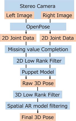
Figure 6 shows the processing flow of the proposed method in which devices or functions are blue-backed and resultant data orange-backed.

Figure 6.

Processing flow of the proposed method.

4. Experiments and discussion

Here we show the stereo camera used and its calibration result, observed joint data, and some preprocessing results for them. Performances of the low-rank filter, spatial AR model, and puppet models are also discussed with the implementation.

4.1 Stereo camera and its calibration

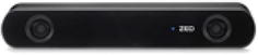
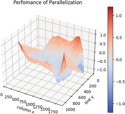
Figure 7 shows the stereo camera we used in the experiments below, and Table 2 shows its specification. The camera was stereo-calibrated so that parallelization was made. We evaluated the performance of the calibration by showing the difference in vertical coordinates between both the stereo-pair images of corner points of a chess board sheet used for the camera calibration as shown in Figure 8. The difference was within plus or minus 0.5 pixels except around the four corners of the image, and we found that the parallelization was achieved with high accuracy.

Figure 7.

A stereo camera Zed2 was used.

Parameter	Value
Number of pixels	3840 × 1080
Format	Side by side
Frames per second	30 fps
Baseline length	120 mm
Field of view	120 degrees

Table 2.

Specification of the stereo camera. *Zed2 originally has higher performance. We used lower mode for easy recording.

Figure 8.

Vertical coordinate differences among all corresponding points in stereo-pair images.

4.2 Data completion and 2D-filtering

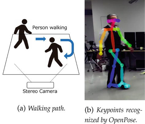
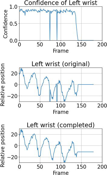
We recorded a person walking in a room illuminated by a ceiling light in a video. He/she walked across the optical axis of the camera at a distance of about 5 [m] in going right and 4 [m] in returning with the same pace as far as possible. We applied OpenPose to get the coordinates of keypoints on the stereo-pair images in each frame as shown in Figure 9. Some of the joint coordinates were missing as we were afraid, so we found the sections having zero confidents and linearly interpolated them by connecting nonzero values at both ends of the sections, as shown in Figure 10. Top of it shows that the confidence falls to zero around 70, 90, and over 140 in frames due to occlusions. The first two of them yield spike-shaped noises and the third zero output in the middle. The bottom shows that the spikes were well interpolated and that the last nonzero value was kept to the end of the data.

Figure 9.

Walking path and an example of recognized keypoints.

Figure 10.

Performance in completing missing data; confidence (top), missing data (middle), and completion result (bottom).

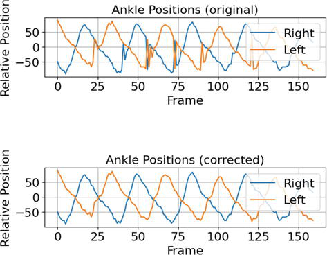
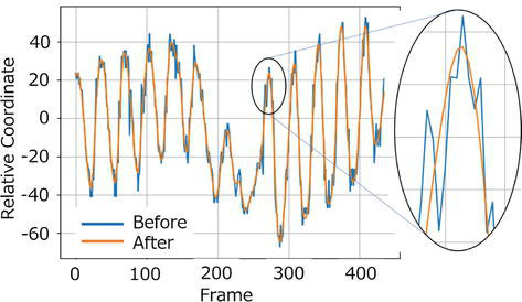
Figure 11 shows an example of the original trajectories of ankles (upper) after the missing value completion and their correction result (lower). The original trajectories included the leg duplications at frames 23–25, 41, 58, 90, and 121, and leg swappings at 56 and 73, respectively. We experimentally determined the threshold as 0.3 and got the best performance. Figure 12 shows the performance of the low-rank filter applied to the time sequence of the right ankle horizontal coordinate. The resultant coordinates were compared with the original ones. After some trials, we set the AR model length as 12 and the rank as unity ($r_f=1$). The low-rank filter provided us the excellent performance in reducing severe noise. The result was smooth and well reproduced the original shape, which cannot be obtained with a simple low-pass filter. Expecting to get something personal feature, we repeated the experiments by increasing the rank up to three. Unfortunately, larger ranks yielded only instability in the pose.

Figure 11.

Correction results for the swappings and duplications; original (upper) and correcting result (lower).

Figure 12.

Performance of 2D low-rank filter applied to the time sequence of the right ankle horizontal coordinates.

4.3 Puppet model fitting

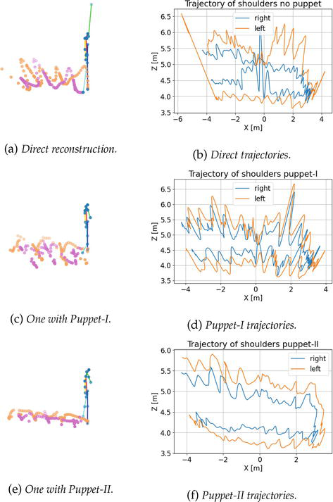
Figure 13 shows the performances of the puppet model fitting for stabilizing the three-dimensional poses reconstructed from the joints on the stereo-pair images. The left row indicates the reconstructed pose with footprints, and the right trajectories of both shoulders are projected on the x-z plane.

Figure 13.

Reconstructions of 3D-pose and shoulder trajectories.

In Figure 13a, although some joints were shifted from their original positions, their overall shape has preserved a human shape. Such discrepancies are considered to be the result of the low-rank filter in the previous stage being independently applied to each joint regardless of the mutual position of the joints. This can also be seen from the fact that the gaps between the two-dimensional trajectories of both shoulders shown in Figure 13b were not constant. The distortion was somewhat compensated by applying puppet-I model as shown in Figure 13c. The model puppet-I acted as a kind of constraint and gave the reconstructed pose a possible positional relationship among the joints as a human. You can see that the shoulder width was corrected to a constant though their positions included larger fluctuation as shown in Figure 13d. The fluctuation indicates that some systematic noise remains in the parallax after fitting the model puppet-I. Although the shoulder width alone is not enough, the puppet-I enabled us to reproduce relative poses from the measured joint coordinates with smoothing by the low-rank filter. We consider that the fluctuations can be reduced by applying a normal low-pass filter, such as a moving average one.

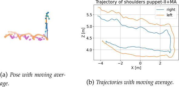
The model puppet-II was developed as the improved version of the puppet-I. This is because puppet-I rarely produces larger distortions that stretch the upper body (shoulders and arms) from the lower body (hips and legs), particularly in an area far from the camera. We speculate that this phenomenon is related to decreasing the precision in OpenPose recognition of joint positions as the object becomes smaller. Therefore, we adopted the rigid body in the puppet-II with some pose stabilizing techniques. Whereas the puppet poses are optimized in the three-dimensional world coordinate system in puppet-I, it is done on the two-dimensional image coordinate system in puppet-II. When a person crosses the optical axis and both shoulders are on it, they appear at the same point on the reference image, and the difference in their parallax is slight. Therefore, noise in the stereo-pair images prevents us to distinguish whether the front of the model is fitted to the front of the object or inverted to fit the back. Since the optimization strongly depended on the initial values, we suppressed the model flip by stabilizing them. The stabilization was performed by fitting the body model in Figure 5a to joint coordinates on not only the target frame but also multiple frames before and after the target frame. The multi-frame fitting was based on the fact that the corresponding point translation on the stereo-pair images with keeping the parallax just produced the translation in the world coordinate system without changing the distance. We translated the body joints on all the frames in the window so that the mid-point between the neck and the mid-hip of them matched that of the target. We set a window w with a width of 24 and used the optimization result for all frames in it as the initial values for optimization in a frame in the central small window containing 12 frames. After finishing the optimization of them, we shifted the window so that the central small window covered frames without gaps. We repeated those procedures until all frames were processed. Before performing the optimization for legs and arms, we applied an inverted test. When the direction from neck to nose in the optimized model did not match that in the measured pose, we flipped the body model. Figure 13e shows one of the resultant poses with footprints and Figure 13f shoulder trajectories. The procedures above were for adjusting the positional relationship among the joints and did not affect smoothing the distance from the camera. Figure 14 shows the result of suppressing the variation in the distance by applying a moving average filter and their shoulder trajectories. We consider that walking human does not make sudden changes in posture for 1/3 of a second and determined the window width as 21.

Figure 14.

Processed 3D-pose and shoulder trajectories with moving average.

4.4 Posterial 3D-filterings

The final processings were three-dimensional low-rank filtering as a smoother in the time domain and spatial AR model filtering as one in the spatial domain. Those filters were applied to the moving average data.

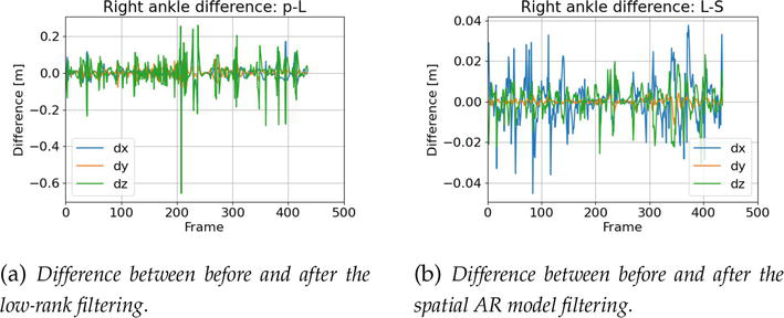
Figure 15a indicates the performance of the low-rank filter LRF-3D separately applied to the time sequence of three-dimensional coordinates of the right ankle, and Figure 15b that of the spatial AR model filter SARF with the rank reduction from 45 to 16 using sequential 7 poses at a time applied to each pose coordinates. Both figures show the differences $\mathit{dx},\mathit{dy},$ and $\mathit{dz}$ in coordinates $x,y,$ and $z$ between before and after applying the filters, respectively. Pulse-shaped noises mainly in the z-coordinates were removed by applying the former filter, and those slightly remaining in the x-coordinates were cut by applying the latter one. The values on the vertical axis in Figure 15b were one digit smaller than those in Figure 15a. This indicates that the previously applied LRF-3D has removed most of the spike-shaped noise. Since the mean value of the difference did not contain a larger bias component, it is suggested that both filters worked to smooth the poses. Figure 16 shows the final results using the models puppet-I and puppet-II, respectively. We applied the same post-processing after the puppet model fitting. In those figures, we also add the footprints and a virtual plane for recognizing the walking trajectory and for comparing their performances.

Figure 15.

Performance of the low-rank filter and the spatial AR model filter.

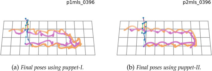
Figure 16.

Final poses with footprints.

In Figure 16a, we see that the puppet-I produced almost the same shape in the pose itself, but slightly disturbed footprints with distorted trajectories from the U-shape. On the other hand, we see that footprints in Figure 16b had a more precise U-shaped trajectory and a regular pattern. These features indicate rhythmic movement of the legs in actual walking was captured well by using the model puppet-II. Therefore, we regard that the model puppet-II has higher performance as a sensing tool, especially in predicting joint positions, in the person walking measurement.

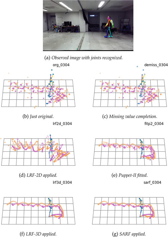
Figure 17 shows intermediate results corresponding to procedures listed in Figure 6. Joints reconstructed from the original data themselves were severely affected by intensive noise and gave us impossible shapes and widely scattered footprints as shown in Figure 17b. Applying the missing value completion did not change the situation as shown in Figure 17c. The impossibilities in joints’ location and scattered footprints were dramatically improved by the low-rank filter LRF-2D, although some unnaturalness remained as shown in Figure 17d. The unnaturalness was removed almost perfectly by predicting and correcting body position with fitting the model puppet-II as shown in Figure 17e. Following the low-rank filter, LRF-3D provided smoothness in joint movements as shown in Figure 17f. The last spatial AR model filter SARF also gave spatial smoothness as shown in Figure 17g, although LRF-3D was so powerful that the effect of SARF was almost invisible. The result indicates that the proposed method measured the person walking almost perfectly in not only its pose but also its position. We also provide the whole scene of the person walking by a video at https://youtube.com/shorts/gvqF3m9xPjk. As can be seen from Figure 16 (and the video), LRF and the puppet-II model performed very well in the walking measurements conducted in this study. The former extracts the dominant mode in the signal, so from the standpoint of the behavior measurement, the longer the same movement lasts (in this case, the more steps taken), the more stable the results will be. On the other hand, if the pose changes significantly in a short period, the dominant mode itself may become unstable and the performance may not be sufficient. We believe that such poor performance may be improved by using a stereo camera with a high frame rate for recording poses. The latter was introduced on the fact that the joint positioning in a person’s upper body (shoulders and hips) does not change significantly with a pose. The good performance of this model can be interpreted as the effect of incorporating already existing knowledge into the measurement. In this case, we believe that the fixed joint positioning as a correlation structure narrows the search area in the optimizing process and thereby improves total accuracy.

Figure 17.

Intermediate results after the main processing steps have been completed.

Now, we consider the applicability of the model puppet-II used here to persons with different heights and body types. Based on the followings, we think the body type is not so much larger problem, and the height difference can be compensated by expanding or shrinking the length of each limb correspondingly to the height. The reasons are that roughly measured limb lengths already gave us almost the perfect results, the model had a very simple structure, and the position and the direction of body parts were determined by an optimization process, not a matching one.

Conventionally, to recognize human behavior, we have to measure poses and analyze the behavior as the temporal change of the poses. In this process, recognizing the human itself was an extremely hard task. Recent advances in deep learning have enabled software systems such as OpenPose to quantitatively extract human joints independently of the observation direction. Analysis with two-dimensional data, however, still depended on the observing direction, and one with three-dimensional data was attractive but some problems also remained in acquiring the three-dimensional human joint coordinates. In this study, we have established a technical basis for quantitatively handling three-dimensional poses and their temporal changes, that is, behavior, by removing the extreme noise in the three-dimensional joint coordinates converted from OpenPose extracting stereo-pair joint coordinates.

5. Conclusions

Based on the fact that human joints did not move at random but moved together with having a kind of spatial correlation structure in each action, a joint-based method was proposed to measure three-dimensional human pose with position in walking as the first step for obtaining the correlation structure. The joint positions were obtained by applying OpenPose to both left and right images acquired with a general-purpose stereo camera. The original three-dimensional joint coordinates were severely affected by missing values and/or positional fluctuation included in two-dimensional coordinates on the stereo-pair images. Since noise in tree-dimensional coordinates caused by Gaussian assumed fluctuation followed a Cauchy distribution, a simple averaging did not smooth the noise well. Focusing on the dominant mode, we succeeded in separating severe noise by lowering the rank of time-series data of the joint coordinates. We called it a two-dimensional low-rank filter LRF-2D. Independent application of LRF-2D to the time series of each joint coordinate yielded some positional distortions in joint locations. Those distortions were corrected by introducing the puppet model. The puppet model was introduced as a kind of restraint from the fact that lengths of the backbone, upper limbs, and lower ones were invariant in actions. Two types of model, flexible puppet and rigid one, were proposed and the rigid puppet model gave us better performance than the flexible one. In the rigid model, locations of both shoulders and hips to the backbone were fixed in the body part of the puppet, and their three-dimensional positions were determined so that the squared sum of differences among their two-dimensional joint coordinates back-projected and observed ones on stereo-pair images fell down the minimum. This meant that the optimum position of the body part was determined from observed two-dimensional joint coordinates while predicting its possible three-dimensional positions using known knowledge. Following the application of LRF-3D to time-series data of joint coordinates and application of the spatial AR model filter SARF to joints in each frame achieved almost the perfect smoothing of the joint movements in walking. The final result represented rhythmic footsteps well. Thus, the model predictive measurement derived us to the success of person walking measurement. In addition, we found that OpenPose had high precision in detecting human joints and high directional reproducibility in recognizing their positions for performing a stereo-vision measurement.

In this study, we have established a technological basis that enables a quantitative understanding of human posture and its temporal changes, that is, positioned behavior, by optical measurement from a remote location. This is expected to advance research on the recognition of human behavior and its application to gait recognition. However, although we evaluated the measurement performance of the pedestrian system qualitatively here, more quantitative evaluation is needed to use the system for applied research. At the same time, a rigorous evaluation is also needed to determine the performance of OpenPose as a human joint recognition tool, including the adoption of another recognition system with higher performance. Another future task is to extract and analyze the spatial correlation structure among all joints in movements such as walking.

Abbreviations

AR	Auto-Regression
JSON	JavaScript Object Notation
LRF	Low-rank filter
LRF-2D	Two-dimensional low-rank filter
LRF-3D	Three-dimensional low-rank filter
SARF