Design of an Adaptive Neuro-Fuzzy Inference System (ANFIS) for Tractor-Implement Tillage Depth Control

Abstract

During ploughing operations, variations in soil conditions cause ploughing depth errors. This chapter presents the designed of a neuro-fuzzy controller to decrease tractors ploughing depth errors. The tractor’s electrohydraulic lifting system consisting of pump, valves and cylinders, position and force sensors, and the neuro-fuzzy controller, is modeled using MATLAB software. The aim of this study is to control the draft force and the position of the lifting mechanism using a controller based on the Adaptive Neuro-fuzzy Inference System (ANFIS). After several simulations, the performance of the proposed controller is analysed and compared with that of a Proportional Integral Derivative (PID) controller and a fuzzy logic controller. The performance index based on the Integral Time Absolute value Error (ITAE) criterion indicates a value of 0.32 in the case of the neuro-fuzzy controller; this is almost half the value of the PID controller, which is 0.76. In addition, the values of the standard deviations on the desired depth for the proposed controller are lower than those obtained by the PID controller and those of the fuzzy controller. The results obtained show that the neuro-fuzzy controller adapts perfectly to the dynamics of the system with rejection of disturbances.

1. Introduction

From the very beginning of our existence, human beings have worked the land and produced their own food to sustain life. Good soil preparation helps crops get off to a good start, improves water infiltration and facilitates root penetration. There is generally a correlation between ploughing depth and crop yield gain. Tractors are the main source of power for ploughing implements. For optimum tractor performance during soil preparation, the tractor’s electro-hydraulic lifting system is used to control ploughing depth [1]. The tractor’s electro-hydraulic lifting system consists of three main parts, namely the three-point hitch mechanism, a hitch control valve, and an electronic control unit. The tractor’s three-point hitch mechanism was invented by Harry Fergusson in 1925 to lift, lower and transport hitched implements. When ploughing, the system remains in a floating position so that the plough operates at a constant working depth and can follow the soil surface even in undulating conditions [2].

On an agricultural tractor, the following operating modes are possible, position control and draft control [1]. Draft control adjusts the depth of the implement under the soil according to the force value from the ground during the tillage process. The force applied from equipment to the tractor depends on the equipment depth, soil characteristics, and vehicle velocity. In the position control, the control system arranges the height of the mechanism according to the given angle input. To improve the control accuracy of a tractor’s electro-hydraulic lifting systems, P. Suomi et al. [2] designed a Proportional Integral Derivative (PID) controller to adjust the seeding depth of a tractor mounted seed drill. However, variations in soil structure were the main cause of system disturbances and errors during seeding. Moreover, the tractor’s electro-hydraulic system is strongly non-linear and time-lag and the PID controller which is linear control, cannot solve the problems. Han et al. [3] designed a fuzzy logic controller to adjust the tillage depth of the implement. This controller made it possible to decrement variations in ploughing depth while increasing the tractor’s tractive efficiency. Subsequently, Shafaei et al. [4] developed a fuzzy controller for ploughing depth as a function of draft force for various agricultural implements. The results indicated that the application of fuzzy controller rather than the standard controller available on the tractor resulted in an increase in tractive efficiency and overall energy efficiency. In addition, ploughing depth error, drive wheel slip and fuel consumption were reduced.

Although the fuzzy controller achieve good control accuracy, there are still some short-comings to overcome, including the designing of fuzzy inference system. The design of fuzzy inference system is based on knowledge acquired by expert operators. However, operators may not be able to translate their knowledge and experience into the form of a fuzzy logic controller. In addition, sometimes the area of expertise is not available. So it would be interesting to have algorithms for automatically learning fuzzy parameters (sets and fuzzy rules). One method for meeting these requirements is the Adaptive Neuro-fuzzy Inference System (ANFIS). This study uses the simulation software to design a neuro-fuzzy controller for tractor’s electro-hydraulic lifting system based on ANFIS.

Indeed, Adaptive Neuro-Fuzzy Inference System (ANFIS) have been widely employed in control engineering with satisfactory in terms of high robustness, easy settling time, zero peaks overflow [5, 6, 7, 8]. The remainder of the chapter is organised as follows. The second section presents the hitch-implement model. The third section describes the electro-hydraulic actuator model. The fourth section presents the control strategy. The fifth section present the MATLAB/Simulink simulation and the obtained results are commented. The last section conclude the chapter.

2. Modelling of hitch-implement mechanism

2.1 Kinematic and dynamic analysis

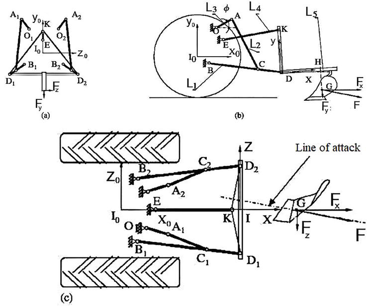
Modelling begins with a kinematic and dynamic analysis of the hitch-implement system. In the study proposed by Bentaher et al. [9], the coordinates of each joint are calculated in the Cartesian reference frame (x_o, y_o, z_o) with I_o, the center of the shaft connecting the rear wheels, as the point of origin. G is the tillage application point. Figure 1 shows the different views of the system to be modelled. In this figure, the lower links are identified by B₁D₁ and B₂D₂ of identical length L₁, the lift rods are identified by A₁C₁ and A₂C₂ of identical length L₂, the lift arms are identified by O₁A₁ and O₂B₂ of identical length L₃, and the upper link is identified by EK of length L₄, rock shaft angular position. The longitudinal component of the (tillage force) draft load is F_x, the vertical component of the draft load is F_y, and the lateral component is F_z.

Figure 1.

Rear view (a), side view (b) and upper view (c) of the hitch-implement system.

To simplify the calculation of forces, the three-point hitch system is modelled by ties and pin joints. The position of the implement on the ground is determined by the following equations:

$$x_G=x_D+\mathit{IH}\left(\frac{y_K-y_D}{\mathit{IK}}\right)+\mathit{HG}\left(\frac{x_K-x_D}{\mathit{IK}}\right)$$E1

$$y_G=y_D-\mathit{HG}\left(\frac{y_K-y_D}{\mathit{IK}}\right)+\mathit{IH}\left(\frac{x_D-x_K}{\mathit{IK}}\right)$$E2

A calculation program is then developed to determine these coordinates. The inputs to this program are the characteristics of the tractor taking into account the Cartesian coordinates of O, B, E, and the parameters L₁, L₂, L₃, L₄, IK, IH, HG.

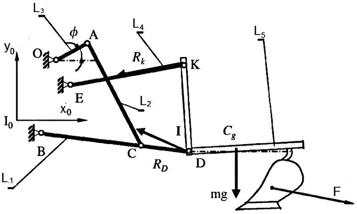
Figure 2 shows the forces acting on the system, Cg and mg are respectively the centre of gravity and the weight of the implement frame, and Ri is the reaction at point i.

Figure 2.

Force diagram of the hitch-implement system.

The equilibrium of the lower left link is determined by the system of equations below:

$${{}^{g}R}_{\mathit{Dx}}+{{}^{g}R}_{\mathit{Bx}}+{{}^{g}R}_{\mathit{Cx}}=0$$

$${{}^{g}R}_{\mathit{Cy}}\left(z_C-z_B\right)-{{}^{g}R}_{\mathit{Cz}}\left(y_C-y_B\right)+{{}^{g}R}_{\mathit{Dy}}\left(z_D-z_B\right)-{{}^{g}R}_{\mathit{Dz}}\left(y_D-y_B\right)=0$$

$${{}^{g}R}_{\mathit{Cx}}\left(y_C-y_B\right)-{{}^{g}R}_{\mathit{Cy}}\left(x_C-x_B\right)+{{}^{g}R}_{\mathit{Dx}}\left(y_D-y_B\right)-{{}^{g}R}_{\mathit{Dy}}\left(x_D-x_B\right)=0$$

$${{}^{g}R}_{\mathit{Cy}}\left(x_C-x_B\right)-{{}^{g}R}_{\mathit{Cx}}\left(z_C-z_B\right)+{{}^{g}R}_{\mathit{Dz}}\left(x_D-x_B\right)-{{}^{g}R}_{\mathit{Dx}}\left(z_D-z_B\right)=0$$

$$\frac{{{}^{g}R}_{\mathit{Cx}}}{\left(x_A-x_C\right)}=\frac{{{}^{g}R}_{\mathit{Cy}}}{\left(y_A-y_C\right)}=\frac{{{}^{g}R}_{\mathit{Cz}}}{\left(z_A-z_C\right)}=\frac{{{}^{g}R}_C}{L_2}$$E3

here, Rij is the reaction at point “i” along the direction “j”, x_i, y_i and z_i are the Cartesian coordinates of point “i” and “g” indicates the left side of the hitch-implement system [9]. The balance of the lower right-hand link is similar (with d for the right-hand side). The system of equations below is derived from the equilibrium position of the implement (Figure 2):

$$\left\{\begin{array}{l}{F}_x={{}^{g}R}_{\mathit{Dx}}+{{}^{d}R}_{\mathit{Dx}}+R_K\left(\frac{x_K-x_E}{L_4}\right)\\ F_z={{}^{g}R}_{\mathit{Dz}}+{{}^{d}R}_{\mathit{Dz}}\\ F_y={{}^{g}R}_{\mathit{Dy}}+{{}^{d}R}_{\mathit{Dy}}+R_K\left(\frac{y_K-y_E}{L_4}\right)+\mathit{mg}\\ z_D\left({{}^{d}R}_{\mathit{Dy}}-{{}^{g}R}_{\mathit{Dy}}\right)=F_z\left(y_G-y_D\right)+\mathit{mg}\left(z_{\mathit{Cg}}\right)\\ \left[\left(y_K-y_D\right)\left(x_K-x_E\right)-\left(x_K-x_D\right)\left(y_K-y_E\right)\right]\frac{R_K}{L_4}=F_x\left(y_G-y_D\right)-F_x\left(x_G-x_D\right)+\mathit{mg}\left(x_{\mathit{Cg}}-x_I\right)\\ F_z=\frac{\left({{}^{d}R}_{\mathit{Dx}}-{{}^{g}R}_{\mathit{Dx}}\right)}{\left(x_G-x_D\right)}{z}_D\end{array}\right.$$E4

Here, F_x, F_y and F_z are the orthogonal components of the draft load at point G. The solutions of these equations give the three orthogonal components of the draft load.

$$\begin{array}{l}{F}_x=\left[\frac{\left(x_K-x_E\right)\left(x_D-x_B\right)\left(y_K-y_D\right)+\left(x_G-x_K\right)\left(x_D-x_B\right)\left(y_K-y_E\right)-\left(x_K-x_E\right)\left(x_G-x_D\right)\left(y_D-y_B\right)}{\left(x_D-x_B\right)\left(y_G-y_D\right)-\left(x_G-x_D\right)\left(y_D-y_B\right)}\right]\\ \times \frac{R_K}{L_4}+\left[\frac{\left(x_C-x_B\right)\left(y_A-y_C\right)-\left(x_A-x_C\right)\left(y_C-y_B\right)}{\left(x_D-x_B\right)\left(y_G-y_D\right)-\left(x_G-x_D\right)\left(y_D-y_B\right)}\right]\frac{\left(x_D-x_G\right)}{L_2}\left[{{}^{g}R}_C+{{}^{d}R}_C\right]\\ +\frac{\left(x_D-x_B\right)\left(x_G-x_{\mathit{Cg}}\right)}{\left(x_D-x_B\right)\left(y_G-y_D\right)-\left(x_G-x_D\right)\left(y_D-y_B\right)}\mathit{mg}\end{array}$$E5

$$\begin{array}{l}{F}_z=\left[\frac{\left(x_C-x_B\right)\left(y_A-y_C\right)-\left(x_A-x_C\right)\left(y_C-y_B\right)}{\left(x_D-x_B\right)\left(y_G-y_D\right)-\left(x_G-x_D\right)\left(y_D-y_B\right)}\right]\frac{z_D}{L_2}\left[{{}^{g}R}_C+{{}^{d}R}_C\right]\\ +\frac{\left(x_B-x_D\right)z_{\mathit{Cg}}}{\left(x_D-x_B\right)\left(y_G-y_D\right)-\left(x_G-x_D\right)\left(y_D-y_B\right)}\mathit{mg}\end{array}$$E6

$$\begin{array}{l}{F}_y=\left[\frac{\left(x_K-x_E\right)\left(y_K-y_G\right)\left(y_D-y_B\right)+\left(x_D-x_K\right)\left(y_K-y_E\right)\left(y_D-y_B\right)+\left(x_D-x_B\right)\left(y_K-y_E\right)\left(y_G-y_D\right)}{\left(x_D-x_B\right)\left(y_G-y_D\right)-\left(x_G-x_D\right)\left(y_D-y_B\right)}\right]\\ \times \frac{R_K}{L_4}+\left[\frac{\left(x_C-x_B\right)\left(y_A-y_C\right)-\left(x_A-x_C\right)\left(y_C-y_B\right)}{\left(x_D-x_B\right)\left(y_G-y_D\right)-\left(x_G-x_D\right)\left(y_D-y_B\right)}\right]\frac{\left(y_D-y_G\right)}{L_2}\left[{{}^{g}R}_C+{{}^{d}R}_C\right]\\ +\frac{\left(x_D-x_B\right)\left(y_G-y_D\right)-\left(x_{\mathit{Cg}}-x_D\right)\left(y_D-y_B\right)}{\left(x_D-x_B\right)\left(y_G-y_D\right)-\left(x_G-x_D\right)\left(y_D-y_B\right)}\mathit{mg}\end{array}$$E7

These equations allow the hitch-implement mechanism to be sized according to the category of tractor. As there is a wide variety of implements, the three-point linkage must be designed taking into account the standards for agricultural machinery, in order to connect each implement smoothly to the tractor [10, 11]. Tractors are divided into four main categories (Table 1), and the design constraints for the three-point hitch mechanism are established according to the tractor category.

Category	Engine Power (kw)
1	Up to 48
2	Up to 92
3	80 to 185
4	150 to 350

Table 1.

Tractor categories [10].

2.2 Computer-aided design

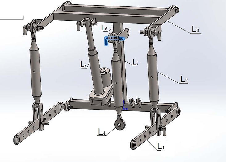
The tractor three-point hitch mechanism was modelled in SolidWorks. The mechanical assembly of the system is shown in Figure 3. The tractor used is a Category 2, with a maximum lifting capacity of 3546 kg and 90 horsepower [10, 12].

Figure 3.

Computer aided design (CAD) of a tractor three-point hitch mechanism.

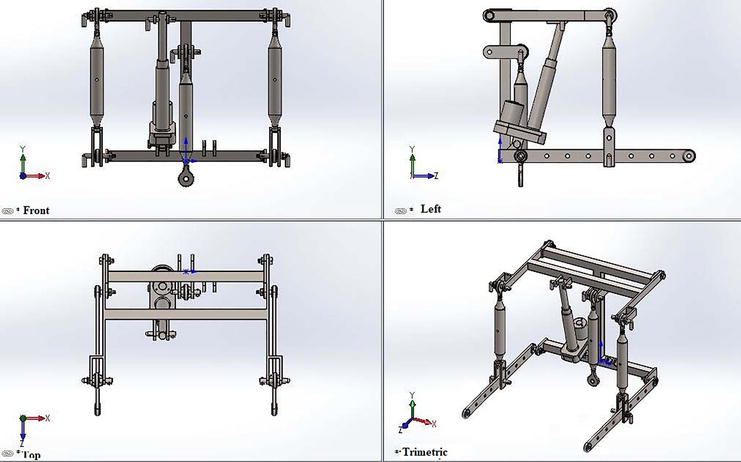
The base of the cylinder is fixed to the main frame of the tractor, its rod to the lifting arm, and it has a total stroke of 180 mm. In the remainder of this work, we use data supplied by the Nebraska Tractor Test Laboratory to design the three-point hitch mechanism [12]. The dimensions of the model are given in Table 2. Figure 4 shows different views of the modelled three-point hitch mechanism.

Part name	Measure
Lower link length (L1)	946 mm
Lift rod length (L2)	765 mm
Lift arm length (L3)	295 mm
Upper link length (L4)	650 mm
Vertical length from upper link pivot point to lower link pivot point (L5)	460 mm
Vertical length from lift arm pivot point to upper link pivot point (L6)	130 mm
External lift cylinder length (L7)	380–560 mm
Stroke of the cylinder	180 mm
Mast Height	610 mm

Table 2.

Three-point linkage parameters [12].

Figure 4.

Front view, left view, top view and trimetric view of the three-point hitch mechanism in SolidWorks.

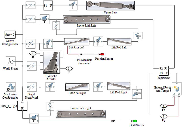
The necessary connections such as cylindrical, revolute and spherical joints are defined in SolidWorks. The CAD model is then exported to MATLAB/Simscape Multibody. This is an XML data file of the Solidworks model. This is done using the “smimport” function. The data in this file contains the block parameters for MATLAB/Simscape Multibody. Since the entire mechanism is exported from SolidWorks, all moments of inertia and masses are taken into account. Once in MATLAB, the implement properties are defined. The MATLAB model of the hitch-implement mechanism is shown in Figure 5.

Figure 5.

Hitch-implement mechanism in MATLAB.

In this work, two implements were used: a chisel plough and a moldboard plough. The parameters of the implement and the soil resistance (draft load) corresponding to each type of soil are provided by ASABE (American Society of Agricultural and Biological Engineers) [13]. The draft load is expressed by:

$$F=T_s\times \left[a+b\times V+c\times V^2\right]\times W_e\times H_d$$E8

with, F the implement draft load (N), T_s the soil texture for a category s. a, b and c are parameters of the second order polynomial fit. a is in N/cm per unit, b is in N/cm per unit per m/s, c is in N/cm per unit per m²/s². V is the tractor speed (m/s). We is the width of the implement (m) or the number of tines. H_d is the ploughing depth (cm).

The Simulink model of the hitch-implement mechanism has four inputs as shown in Figure 5. Ports B and R are the inlets through which the oil supplied by the hydraulic valve drives the cylinder. The other two inputs are the components of the draft load (F_x and F_y), its represent the disturbances due to the structure of the ground, acting on the implement (Table 3). As lateral forces are neglected, the z axis is not taken into account. The Simulink model has two outputs. The red block represents the signal from the lifting arm and the green block represents the signal from the lower links. The resistance of the soil imposes a significant draft load on the tractor. This draft force is measured using sensors located on the lower links. The position of the implement is measured using sensors located on the lifting arms. The hitch-implement mechanism is controlled by interpreting the values measured by these sensors. Table 3 shows the parameters of the implement used; details of the variables can be found in [13].

Parameters	Chisel plough	Moldboard plough
ploughing depth(cm)	30	10
Weight (kg)	380	200
A	107	116
B	6.3	0
C	0	2.3
Soil type	clay	Fine
Working width (m)	2.1	1.04
Tractor speed(km/h)	7	5
Draft force (N)	8095	2429
Draft range (%)	50	40

Table 3.

Implement and field parameters [13].

3. Modelling the electro-hydraulic system

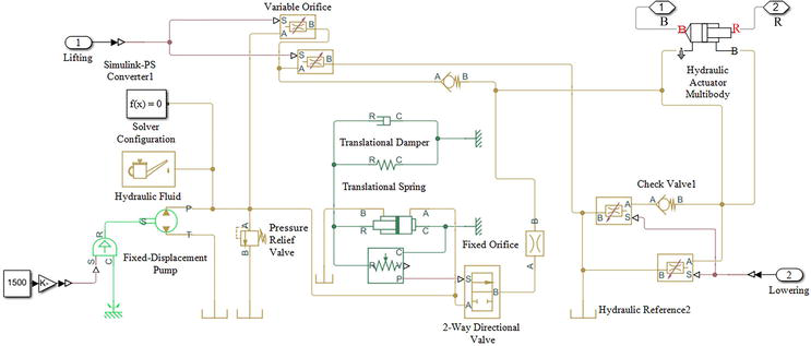
The actuator of the hitch-implement mechanism is the tractor’s electrohydraulic system (Figure 6). It comprises three main parts: a hydraulic pump, a servo-valve and a cylinder. Two signals act on the valve coils to open and close the servo-valve ports. Ports B and R are the outputs from the actuator to the hitch-implement mechanism.

Figure 6.

Tractor’s electrohydraulic hitch system.

3.1 Pump modelling

The tractor engine drive the pump at 1500 rpm. It supplies a flow rate of 60 l/min. The pressure is limited to 194 bar with a pressure limiter fitted to the main distribution block limits. Table 4 gives the parameters of the pump used.

Description	Symbol	Value	Unit
Pump displacement	Cyl	25,4	cm^3/tr
Maximum system pressure	pm	194	bar
Maximum engine speed	ωm	2300	tr/min
Pump/motor ratio	K	1,08

Table 4.

Hydraulic pump parameters.

The flow rate of the hydraulic circuit (Q) is expressed as follows:

$$\mathrm{Q}\left(\mathrm{l}/min\right)={\mathrm{C}}_{\mathrm{yl}}\left({\mathrm{cm}}^3/\mathrm{tr}\right)\times \omega \left(\mathrm{rpm}\right)/1000$$E9

Oil is one of the most critical parameters in a hydraulic system. Depending on the specification of the oil, the characteristics of the system could be radically altered. Most tractor manufacturers recommend Opet Fulltrac Fluid X 10 W-30 hydraulic oil [14]. Since the specifications of SAE30 oil are very similar to those of Opet Fulltrac Fluid X 10 W-30 oil, SAE30 oil is chosen as the system oil in Simulink.

Once the hydraulic flow has been pressurised using the pump, it is routed to the servo-valve along a line. To control the hydraulic flow, a servo-valve is used in the system. On the tractor, the servo-valve controls are electrics.

3.2 Modelling the lift valve

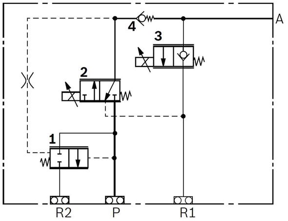
The BOSCH EHR5 type, two-module servo-valve is used to direct the flow of oil from the pump to the cylinder [15]. Figure 7 shows the hydraulic circuit of the valve. The pressure compensator (1), the lifting module (2), the lowering module (3) and the non-return valve (4) are the valve components. With A the oil line from the valve to the cylinder, P the line from the pump to the valve, R₁ the line allowing the return of oil from the cylinder to the tank, R₂ the line allowing the return of valve oil from the compensator to the tank.

Figure 7.

Hydraulic circuit of the BOSCH EHR5 valve [15].

3.2.1 Modelling the pressure compensator

The compensator (1) is a 2-position 2-way hydraulic operation actuator spring-actuated directional control valve. It is usually closed with the help of the spring. When the pressurised oil passing line A and reaches the compensator (1), without any signal, the compensator valve (1) is closed with the help of the spring. Then, pressurised fluid cannot pass the valve and cannot reach the tank [15]. The compensator only acts on the lifting module. The lowering module has no compensator. In fact, the lifting mechanism moves downwards using the weight of the implement and/or external forces such as the draft load. This system is modelled in MATLAB/Simulink. The maximum travel of the valve is 10 mm. The orifice opening are is computed as follows:

$$\mathrm{h}={\mathrm{x}}_0+\mathrm{x}$$E10

Where h is the orifice opening, x₀ the initial opening, x control member displacement from initial position.

3.2.2 Modelling the lifting module

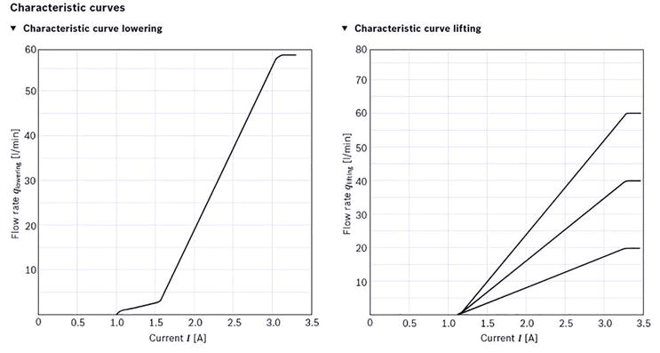
Lifting module (2) is a 2-position 3-way solenoid actuator spring-actuated direction a control valve. Typically, if an electrical signal is not given to the solenoid of the valve, pressurised fluid does not pass through the lifting module. If the electrical input is given to the solenoid, then the solenoid opens gradually according to the value of the given electrical signal current [15]. Meanwhile, lifting module solenoid takes the electrical signal only from lifting the current signal, which comes through controller. The characteristic curves of the lifting and lowering module are shown in Figure 8. The solenoid valve of the lifting module is initially closed with a stroke of 1 mm, and its maximum opening is 3.5 mm.

Figure 8.

Characteristic curves of the lifting and lowering modules [15].

The orifice openings are computed separately for each flow path in terms of the respective opening offset:

$${\mathrm{h}}_{\mathrm{PA}}={\mathrm{h}}_{{\mathrm{PA}}_0}+\mathrm{x}$$E11

$${\mathrm{h}}_{\mathrm{AT}}={\mathrm{h}}_{{\mathrm{AT}}_0}‐\mathrm{x}$$E12

where h_PA and h_AT are the orifice openings of the P-A and A-T flow paths. h_PA0 and h_AT0 are the opening offsets of the P-A and A-T flow paths. x is the spool displacement relative to what in the zero-offset case is a fully closed valve.

3.2.3 Modelling the lowering module

The logic of the lowering module (3) is almost similar to that of the lifting module. It is initially closed with a stroke of 1 mm, and its maximum opening is 3.5 mm.

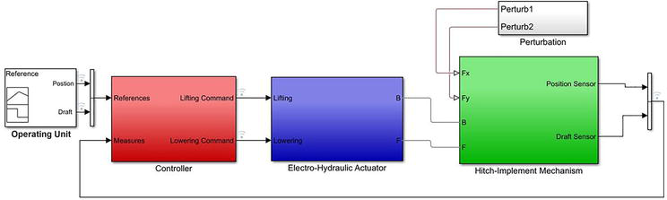
The schematic diagram of a tractor’s electrohydraulic lifting system is a closed-loop system (Figure 9). The first block is the operating unit, where control values are recorded. The red block is the tractor’s electronic control unit. The control deviation resulting from the target/actual comparison is processed in the control unit and transmitted to the hitch control valve. The blue block contains the electrohydraulic actuator, where the hydraulic pump delivers a flow of oil to the hitch control valve, which in turn actuates the hitch cylinder. In the green block, the hitch cylinder acts on the lift arm so that implements can be lifted, held or lowered. The position sensor signal and the draft sensor are the feedback elements of the mechanism.

Figure 9.

Block diagram of the tillage depth control system.

4. Controller design

4.1 Mixed position-force control strategy

Position control involves adjusting the height of the implement above the ground, according to Eq. (13):

$$e=H_d-H_m$$E13

with e the depth deviation, H_d the desired depth and H_m the measured depth.

Force control consists of adjusting the height of the implement as a function of the draft load, using Eq. (13):

$$H_d=\frac{F}{T_s\times \left[a+b\times V+c\times V^2\right]\times W_e}$$E14

The depth deviation can be expressed using Eq. (13):

$$e=\frac{F_d-F_m}{T_s\times \left[a+b\times V+c\times V^2\right]\times W_e}$$E15

with e the depth deviation, F_d the desired force and F_m the measured force.

Here, the participation ratio of desired position and force is adjusted according to the mixing coefficient (M). The deviation in ploughing depth in mixed control can be written as follows:

$$e=\left(\frac{F_d-F_m}{T_s\times \left[a+b\times V+c\times V^2\right]\times W_e}\right)M+\left(H_d-H_m\right)\left(1-M\right)$$E16

When the mixing coefficient M = 0, the system is in “position control” mode; when M = 1, the system is in “draft control” mode; when 0 < M < 1, the control mode is mixed.

4.2 Design of the neuro-fuzzy adaptive controller

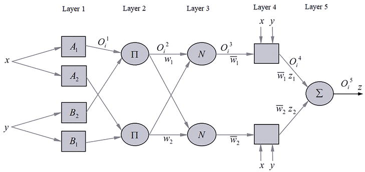
The general architecture of the Adaptive Neuro-Fuzzy Inference System (ANFIS) comprises 5-layer neural network, where each layer corresponds to the realisation of a step in a Takagi Sugeno-type fuzzy inference system [16]. For simplicity, we assume that the fuzzy inference system has two inputs x and y, and z as its output (Figure 10).

Figure 10.

ANFIS system architecture [16].

The first layer enables the fuzzification of inputs x and y. Each neuron i in this layer corresponds to a linguistic variable. The inputs x and y are fuzzified using the membership functions of the linguistic variables A_i and B_i, (generally of triangular, trapezoidal or Gaussian form). Gaussian membership functions are defined by:

$${\mu }_{A_i}\left(x\right)=exp\left(-\frac{{\left(x-c_i\right)}^2}{2{a_i}^2}\right)\mathit{\text{for}}i=1,2$$E17

where c_i is the center and a_i the width of the membership function. These parameters are called “premises”. The outputs of the first layer are as follows:

$$O_i^1={\mu }_{A_i}\left(x\right)$$E18

with ${\mu }_{A_i}\left(x\right)$ the degree of membership of the value x.

The second layer receives the output of each fuzzification node and calculates its output value using the product operator. This operator uses the derivability constraint to deploy the learning algorithm, with each node performing a fuzzy T-norm. The outputs of this layer are the rule weights, obtained by:

$$O_i^2=w_i=min\left\{{\mu }_{A_i}\left(x\right),{\mu }_{B_i}\left(y\right)\right\}\mathit{\text{for}}i=1,2$$E19

The third layer normalises the results provided by the previous layer. The results obtained represent the degree of involvement of the value in the final result.

$$O_i^3=\overline{w_i}=\frac{w_i}{{\sum }_{i=1}^2{w}_i}$$E20

The fourth layer is linked to the initial inputs. The result is calculated as a function of its input and a first-order linear combination of the initial inputs (Takagi - Sugeno approach). This is the defuzzification phase.

$$O_i^4=\overline{w_i}{z}_i=\overline{w_i}\times \left(p_{i}x+q_{i}y+r_i\right)$$E21

where $\overline{w_i}$ is the output of the third layer, $p_i,q_i\mathit{et}{r}_i$ and are parameters referred to as: consequents.

The output layer consists of a single neuron that calculates the sum of the signals from the previous layer, so:

$$O_i^5=\sum _{i=1}^2\overline{w_i}{z}_i$$E22

From the proposed architecture, we can see that there are two layers with adaptive parameters. Initially, the non-linear premises parameters (a_i, c_i) in layer 1, decide on the shape and position of the membership functions, and finally, the consequent parameters (p_i, q_i, r_i) realise a first-order linear combination of the initial inputs. These parameters are updated to minimise errors, using various learning algorithms like gradient descent only, Gradient descent and least-squares estimation (hybrid algorithm). In fact, the hybrid learning approach converges much faster than others. For this reason, it is this approach that we develop in the remainder of this work.

The MATLAB/Simulink environment was used to create, train and test the ANFIS model. First of all, the data for training and testing had to be loaded into the anfis editor. To this end, a PID controller is designed and applied to the system in order to obtain a set of input and output data for training. The parameters of the designed PID controller when the implement is lifted and when the implement is lowered are summarised in Table 5.

Parameters	lifting	lowering
kp	1,22	0,612
Ki	0	0
Kd	0	0,174

Table 5.

PID controller parameters.

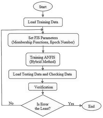
Before training in MATLAB/neurofuzzy, the data are divided into a three-dimensional vector, with 15% of the data set used for testing, 15% are used for verification, and 70% for training. Then, for the two inputs (e and ce), the initial membership functions are chosen. We then define the number of iterations and the desired learning error. Once these parameters have been defined, training can begin. Using a hybrid least-squares and back-propagation gradient descent algorithm method, MATLAB constructs a suitable Fuzzy Inference System (FIS). Figure 11 shown he flowchart for the ANFIS method.

Figure 11.

Flowchart of the ANFIS method.

The hybrid algorithm performs a number of loops to minimise the error on the training data. A series of tests are carried out until an optimal architecture is obtained. The test results are summarised in Table 6.

Membership function	Learning square error	Test square error	Number of iterations
Triangular	3.9%	4.4%	56
Trapezoidal	1.2%	1.9%	37
Gaussian	0.28%	0,31%	20
Gaussian2	0,28%	0,30%	80

Table 6.

Architectures obtained after various trials.

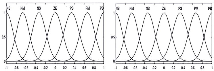
After several trials and 20 iterations, a suitable neuro-fuzzy controller was obtained. The neuro-fuzzy controller obtained has seven Gaussian combination membership functions for the two inputs. After training, the error tolerance is close to zero. The membership functions obtained are shown in Figure 12.

Figure 12.

Membership functions after learning.

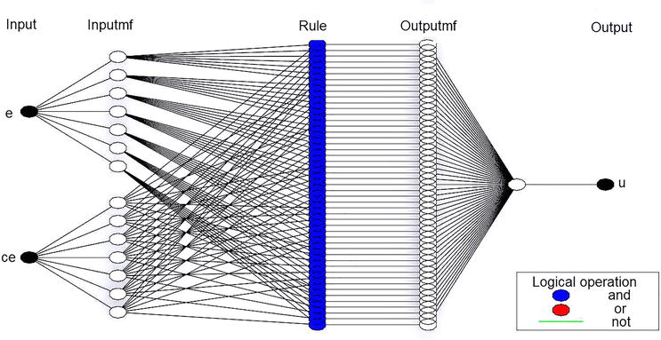
The structure of the resulting neuro-fuzzy controller is shown in Figure 13 with:

• input: representing the two input variables (e) and (ce);

• inputmf: representing the membership functions of seven fuzzy sets for each input;

• rule: evokes and normalises the weights of the rules;

• outputmf: representing the defuzzification stage and the last layer gives the sum of all the data.

Figure 13.

Structure of the developed neuro-fuzzy controller.

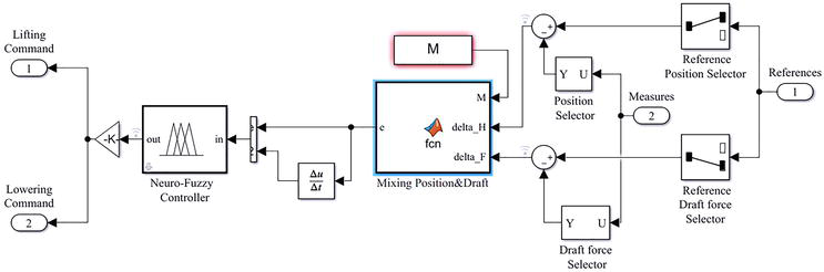
Figure 14 illustrates the principle of the proposed controller. The user enters the parameters of the desired depth Hd, the mixing coefficient M and the desired draft force Fd, from the operating unit. The signals from the force sensor and the position sensor are measured on the hitch mechanism and compared with the desired parameters. The ‘mixing position and draft’ module collects the above signals and uses Eq. (16), to calculate the deviation in depth e. From the deviation in depth e and its derivative ce, the ‘neuro-fuzzy’ module then sends the corresponding command value to the electrohydraulic valve which adjusts the working depth. To lift the implement, a positive signal is sent to the solenoid of the valve and the lifting valve control signal must be within an operating range of 1 to 3.35 A. A negative signal is sent to the solenoid of the valve to lower the implement, and the lowering valve control signal must be within an operating range of −1 to −3.35 A.

Figure 14.

Schematic diagram of the controller.

5. Analysis and interpretation of results

In this section, simulation tests are provided to show the effectiveness of the proposed neuro-fuzzy controller. The working depth errors during tillage operations with chisel and moldboard ploughs are examined. Chisel ploughs are designed for primary tillage with working depths of up to 45 cm. Moldboard ploughs are designed for soil tilth and seedbed preparation. Using the data in Table 3, the disturbance forces due to soil structure are of the order of $\pm 4048N$ for chisel plough, and for moldboard plough.

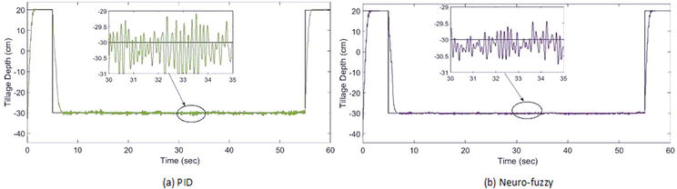
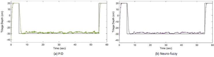
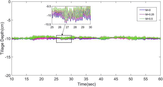
Simulation scenarios are carried out (Figures 15–17) on the chisel plough for different values of mix coefficient M, when the desired ploughing depth is 30 cm. Figure 15 illustrates the variations around the desired working depth under PID and neuro-fuzzy control for M = 0. Between the instants t = 5 s and t = 55 s, the implement shows more variation around the desired working depth under PID control than under neuro-fuzzy control. This is due to the faster response of the neuro-fuzzy controller. Comparisons of the performance of the different controllers are summarised in Table 7. As shown in Table 7, ploughing depth error under neuro-fuzzy control has a maximum value of 0.85 cm. this value is significantly reduced compare to the PID controller, which indicate a maximum ploughing depth error value of 1.61 cm.

Figure 15.

Position of chisel plough for M = 0.

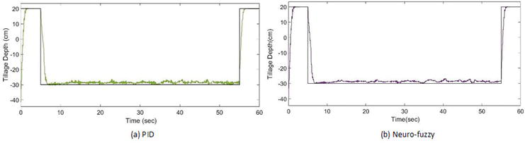
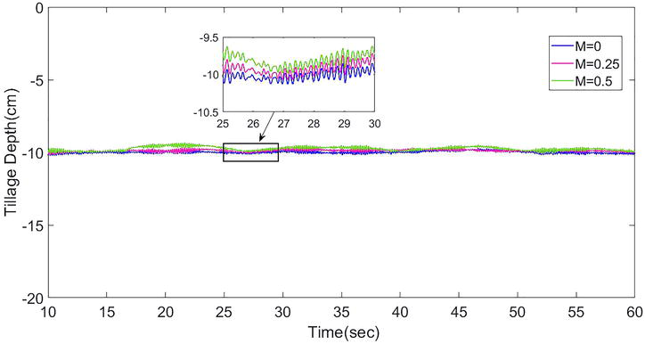
Figure 16.

Position of chisel plough for M = 0.25.

Figure 17.

Position of chisel plough for M = 0.5.

Implement	Controller	M value	Depth mean	min	max	Standard deviation	ITAE
Chisel plough	Neuro-fuzzy	M = 0	29.88	29.07	30.85	0.25	0.32
		M = 0.25	28.68	27.01	30.23	0.54	2.02
		M = 0.5	28.29	26.43	30.28	0.64	2.45
	PID	M = 0	29.47	28.92	31.61	0.45	0.76
		M = 0.25	27.96	26.9	30.70	0.77	2.27
		M = 0.5	27.67	26.22	30.96	0.78	2.71
Moldboard plough	Neuro-fuzzy	M = 0	9.94	9.66	10.18	0.09	0.11
		M = 0.25	9.84	9.51	10.23	0.11	0.41
		M = 0.5	9.69	9.23	10.08	0.17	0.65
	PID	M = 0	9.93	9.28	10.52	0.20	0.23
		M = 0.25	9.83	9.15	10.52	0.21	0.63
		M = 0.5	9.68	8.95	10.34	0.25	0.86

Table 7.

Performances of the different controllers.

Figure 16 shows the position of the chisel plough for M = 0.25. It can be seen that the ploughing depth errors increase. This is confirmed in the illustrations of Figure 17, where the ploughing errors are considerably greater. This can be justified by the fact that when the coefficient M increases, the controller takes into account the draft load as shown in Eq. (16), so the implement becomes more sensitive to soil resistance. This sensitivity is beneficial in limiting wheel slip, but the implement moves away from the desired depth when M > 0.5.

Figure 18 shows the variations around the desired working depth (10 cm) of the mouldboard plough under PID control, for M = 0, M = 0.25, and M = 0.5. We note that there is no significant variation as the M coefficient increases. This is due to the fact that, at shallow ploughing depths, soil resistances are reduced. Figure 19 illustrates the positions of the mouldboard plough under neuro-fuzzy control. With reference to Table 7, for moldboard plough, the minimal standard deviation in ploughing depth was obtained in the cases of the neuro-fuzzy control. This leads to the conclusion that, whatever the type of implement used, the neuro-fuzzy controller offers a faster response and enables the implement to follow the desired working depth more accurately.

Figure 18.

Moldboard plough position under PID control.

Figure 19.

Moldboard plough position under neuro-fuzzy control.

In this work, we use the Integral Time Absolute value Error (ITAE) criterion, to evaluate the proposed neuro-fuzzy controller. We consider the ITAE criterion defined by:

$$\mathit{\text{ITAE}}=\underset{0}{\overset{\infty }{\int }}t\left|e\left(t\right)\right|\mathit{dt}$$E23

As shown in Table 7 the ITAE values of the neuro-fuzzy controller are lower than those obtained by the PID controller. The average working depth values reported in Table 7 indicate that the neuro fuzzy controller considerably reduced ploughing errors. From the observations below, we can conclude that the system offers a great robustness against perturbations and a better stability using the neuro-fuzzy controller rather than the PID controller.

The results obtained in this work are compared with those obtained in the literature. Indeed, this problem is addressed by the authors using a fuzzy logic controller on the tractor’s electro-hydraulic lifting system. These results are reproduced here and compared with the results found by the Neuro-fuzzy controller (Table 8).

Reference	Controller	Implement	Depth mean	Standard deviation
Han et al. [3]	Fuzzy	—	99,33%	0,66
Shafaei et al. [4]	Fuzzy	Moldboard plough	85,05%	0,78
		Chisel plough	89,17%	0,87
Current study	Neuro-fuzzy	Moldboard plough	99,6%	0,25
		Chisel plough	99,4%	0,11

Table 8.

Comparison with previous works.

6. Conclusion

This chapter gives detailed information about the design of an adaptive neuro-fuzzy controller for the tractor’s electro-hydraulic lifting system. Mainly, it focusses on the modelling and analysis of the hitch-implement mechanism, modelling of the hydraulic system, controller design, and simulations of the overall system. On the tractor’s electro-hydraulic lifting system, changes in hydraulic cylinder thrust impose changes in working depth values. The results of the selected scenarios showed that the proposed neuro-fuzzy controller can achieve the desired working depth even under disturbing effects with different ploughing depths and implements. However, the effect of applying the neuro-fuzzy controller for ploughing operations on fuel consumption, drive wheel slip, energy efficiency and forward speed was not analysed in this work. These parameters should be taken into account in future work. In addition, to improve the accuracy of the tractor’s electrohydraulic lifting system, control of hydraulic pump pressure and flow rate should become a future trend.

Conflict of interest

The authors declare that there is no conflict of interests regarding the publication of this chapter.

References

1.Bhondave B, Ganesan T, Varma N, Renu R, Sabarinath N. Design and development of electro hydraulics hitch control for agricultural tractor. SAE International Journal of Commercial Vehicles. 2017;10:405-410
2.Suomi P, Oksanen T. Automatic working depth control for seed drill using ISO 11783 remote control messages. Computers and Electronic in Agriculture. 2015;116:30-35
3.Han J, Xia C, Shang G, Gao X. In-field experiment of electro-hydraulic tillage depth draft-position mixed control on tractor. IOP Conference Series: Materials Science and Engineering. 2017;274
4.Shafaei SM, Loghavi M, Kamgar S. A practical effort to equip tractor-implement with fuzzy depth and draft control system. Engineering in Agriculture Environment and Food. 2019;12:191-203
5.Subha S, Nagalakshmi S. Design of ANFIS controller for intelligent energy management in smart grid applications. Journal of Ambient Intelligence and Humanized Computing. 2020;11(n 6):1-11
6.Shanthi R, Kalyani S, Devie et PM . Design and performance analysis of adaptive neuro-fuzzy controller for speed control of permanent magnet synchronous motor drive. Soft Computing. 2021;25(n 2):1519-1533
7.Saadat SA et al. Adaptive neuro-fuzzy inference systems (ANFIS) controller design on single-phase full-bridge inverter with a cascade fractional-order PID voltage controller. IET Power Electronics. 2021;14:1960-1972
8.Oladipo S, Sun Y. Enhanced adaptive neuro-fuzzy inference system using genetic algorithm: A case study in predicting electricity consumption. SN Applied Sciences. 2023;5:186
9.Bentaher H, Hamza E, Kantchev G, Maalej A, Arnold W. Three point hitch mechanism instrumentation for tillage power optimization. Biosystems Engineering. 2008;100:24-30
10.International Organization for Standardization. GOST ISO 730-2019 Agricultural Wheeled Tractors-Rear Mounted Three-Point Linkage - Categories 1N, 1, 2, 3N, 3, 4N and 4. Geneva; 2020
11.Attachment TF, Implements H, Tractors AW. ASAE S217.12 three-point free-link attachment for hitching implements to agricultural wheel tractors. Power. 2001;1
12.University of Nebraska. Nebraska Tractor Test Laboratory, Nebraska Summary: S706 Massey Ferguson 5460. Lincoln, Nebraska: University of Nebraska; 2009
14.Cad FKG, Plaza EC. Fulltrac Fluid X10W-30 High Protection for Transmissions of Tractor and Agricultural Machines. Istanbul; 2021. Available from: https: //www.opetfuchs.com.tr/content/pdf/tds_fulltrac_X_10w30
15.Bosch Rexroth AG. Hitch Control Valves EHR5-OC, EHR5-LS, EHR23-EM2 RE. 2020. Available from: https://www.naptechniek.nl/images/catalogus/pdf/EHR23_re66125_2013-07.pdf
16.Jang JS. ANFIS: Adaptive-network-based fuzzy inference system. IEEE Transactions on Systems, Man, and Cybernetics. 1993;23(3):665-685
Written By
Aristide Timene, Ndjiya Ngasop and Haman Djalo
Submitted: 18 September 2023Reviewed: 01 October 2023Published: 13 February 2024
Open access peer-reviewed chapter