Evaluating Satellite Image Classification: Exploring Methods and Techniques

Abstract

Satellite image classification serves a critical function across various applications, from land cover mapping and urban planning to environmental monitoring and disaster management. In recent years, significant advancements in machine learning and computer vision, coupled with increased accessibility to satellite imagery, have driven considerable progress in this field. Classification techniques for satellite imagery can be primarily divided into three key approaches: automatic, manual, and hybrid. Each approach offers unique advantages but also comes with its own set of limitations. While most methodologies gravitate toward automatic techniques, choosing an appropriate method should be a carefully considered decision based on specific needs. This paper provides an exhaustive review of cutting-edge classification algorithms, including Artificial Neural Networks (ANNs), Classification Trees (CTs), and Support Vector Machines (SVMs). It also offers a comparative analysis between these modern methods and traditional techniques, focusing on their respective performance metrics when applied to satellite data. This study examines key factors affecting remote sensing data classification, including classifier parameter adjustments and combining multiple classifiers. It reviews existing literature to enhance feature selection and classifier optimization for better accuracy. However, it also points out the continuous need for research in image processing to improve classification accuracy.

1. Introduction

Satellite image classification is a crucial element in the fields of remote sensing and Earth observation. It has a wide array of applications, including but not limited to land cover mapping, environmental monitoring, disaster management, urban planning, and agricultural assessment [1]. Essentially, the classification process categorizes pixels or regions within satellite images into predefined classes or land cover types. This enables the extraction of vital information about the Earth’s ever-changing features [2], serving as a foundation for data-driven decisions across various sectors—from climate change mitigation and resource management to humanitarian efforts [1]. Recent advancements in technology have dramatically transformed the landscape of satellite image classification. The introduction of high-resolution satellites and the increasing availability of multispectral and hyperspectral data have set the stage for a new era in this field [3]. These advances allow for the incorporation of sophisticated machine learning and deep learning algorithms, which substantially enhance feature extraction and enable more context-sensitive classifications [3]. In this evolving context, the critical evaluation of classification methodologies has gained heightened importance. Robust and reliable evaluation frameworks are indispensable for assessing the performance of various classification models, ensuring that the insights garnered are both accurate and actionable [3]. This paper aims to offer a thorough analysis of the evaluation methodologies and techniques currently prevalent in the field. It also provides an overview of contemporary trends, challenges, and innovations in satellite image classification [4]. By examining existing studies, we aim to present a comprehensive perspective on cutting-edge methods, unresolved challenges, and emerging directions in evaluation techniques within this domain. The primary goal of this review is to assist analysts, especially those new to the dynamic world of remote sensing, in making well-informed choices when selecting appropriate classification methods. This will, in turn, lead to more accurate satellite image classifications and the generation of precise Land Use and Land Cover (LULC) maps [3]. In particular, this review focuses on groundbreaking advances in classification algorithms, especially Artificial Neural Networks (ANNs), Classification Trees (CTs), and Support Vector Machines (SVMs). These state-of-the-art techniques have shown considerable promise in the realm of satellite image classification, opening new pathways for enhancing both accuracy and robustness.

1.1 Setting the context for satellite image classification

Satellite image classification sits at the intersection of remote-sensing technology, artificial intelligence, and Geographic Information Systems (GIS). With Earth-monitoring satellites generating vast quantities of data daily, the need for automated techniques to extract valuable insights from this imagery has never been more pressing. These images encompass a range of spectral bands—including optical, infrared, and radar—all of which provide unique and comprehensive data on Earth’s terrestrial and aquatic features. The primary objective of satellite image classification is to transform raw satellite data into actionable intelligence. This involves the identification and categorization of various objects or land cover types, such as forests, urban areas, water bodies, and agricultural fields. This categorization serves as a vital foundation for numerous applications in diverse fields. Whether the focus is on urban planning, precision agriculture, emergency response, or environmental monitoring, the insights derived from accurate satellite image classification are invaluable.

1.2 Satellite image classification techniques

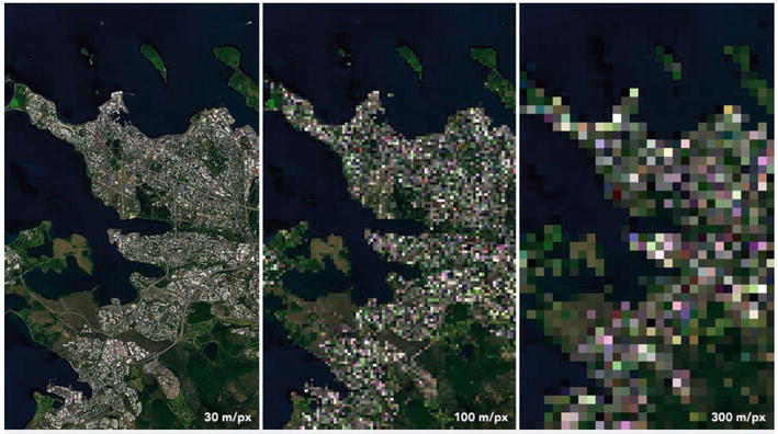
Satellite images can typically be classified into three main categories based on spatial resolution: low-, medium-, and high-resolution. These categories are determined by the pixel size or granularity of the images, which directly influences both the level of detail captured and the suitability of the images for various applications (see Figure 1). Low-resolution images feature coarser pixels and, as a result, cover extensive geographic areas but provide limited detail. Medium-resolution images offer a middle ground, capturing a moderate level of detail while still encompassing relatively large areas. In contrast, high-resolution images are characterized by fine pixels that capture intricate details, making them ideal for specialized and precise analyses. Understanding these distinctions is crucial for selecting the most appropriate type of satellite imagery to meet specific remote-sensing goals and geospatial analysis requirements.

Figure 1.

High, medium and low spatial resolution satellite images.

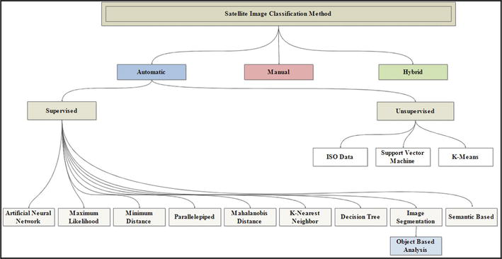
The classification of satellite images is organized into a diverse array of methods and techniques, offering a structured approach to data analysis (refer to Figure 2). Typically, these methods fall under three major categories, each with its own distinctive features and use cases: A. Manual classification, B. Automatic classification, and C. Hybrid classification.

Figure 2.

Hierarchy of satellite image classification techniques [5].

1.2.1 Manual classification

Manual classification techniques are esteemed for their reliability, efficiency, and effectiveness. They rely heavily on the interpretative skills of analysts who leverage their extensive knowledge of local conditions and the unique characteristics of the study area. However, it is crucial to recognize that manual classification can be resource-intensive, often requiring the expertise of field specialists for optimal accuracy. In this approach, the quality and reliability of the classified data are intrinsically linked to the analyst’s skill set and familiarity with the specific area of study.

1.2.2 Automatic classification

While manual classification is closely tied to the expertise of the analyst, automatic classification methods offer an alternative that mitigates this variable. These techniques categorize pixels based on quantifiable metrics like similarity and dissimilarity. Depending on the spatial resolution of the images, automatic classification can be broken down into three distinct categories: (a) pixel-based classification, which focuses on individual pixels; (b) sub-pixel-based classification, which examines fractions of a pixel; and (c) object-based classification, which considers groups of pixels as single entities.

1.2.2.1 Pixel-based classification

Pixel-based techniques form the bedrock of remote-sensing image analysis. These methods operate under the assumption that each pixel in an image corresponds to a uniform land use or land cover type [6]. Within this framework, remote-sensing data are treated as an array of unique pixels, each defined by specific spectral features and associated variables. Generally speaking, pixel-based classification can be divided into two principal groups:

1.2.2.1.1 Unsupervised classification

Unsupervised classification techniques segment an image into distinct classes based on the natural clustering of pixel values, without requiring prior knowledge or training data. Notable algorithms in this category include K-Means and its variant, ISODATA (Iterative Self-Organizing Data Analysis Technique). More recent developments have adapted algorithms like Support Vector Machines (SVMs) and hierarchical clustering methods for unsupervised purposes [7]. However, these methods come with their own set of challenges, such as computational intensity, particularly when handling large datasets. Another limitation is the often-limited accuracy in generating meaningful and specific class distinctions, which may require additional post-processing or user intervention.

1.2.2.1.2 Supervised classification

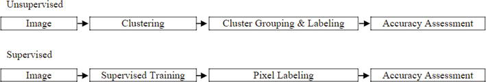
In supervised classification, as illustrated in Figure 3, satellite images are classified using predefined input or training data. An analyst carefully selects representative areas with known class types, commonly referred to as training samples or signatures. The spectral characteristics of individual pixels within the image are then compared against these training samples. Based on predefined decision rules, the analyst categorizes each pixel into the most appropriate class [8]. Over the years, a diverse array of supervised classification techniques have emerged, enriching the framework for satellite image classification, as further detailed in Figure 3.

Figure 3.

The major steps of supervised and unsupervised image classification.

1.2.2.2 Sub-pixel-based classification

Traditional pixel-based methods commonly operate on the premise that each pixel in an image exclusively represents one type of land use or land cover. This assumption becomes less sustainable when working with medium or coarse spatial resolution satellite images due to the inherent heterogeneity of natural landscapes [9]. Sub-pixel-based classification techniques present a more nuanced solution by precisely quantifying the distribution of various land use or land cover types within each pixel [10]. Leading techniques in this category include fuzzy classification, neural networks [11], regression modeling [12], regression tree analysis [13], and spectral mixture analysis [14]. Engineered to address the challenges of heterogeneous pixel compositions, these methods offer a refined way to capture the diversity of land use and land cover types within a single pixel.

1.2.2.3 Object-based classification

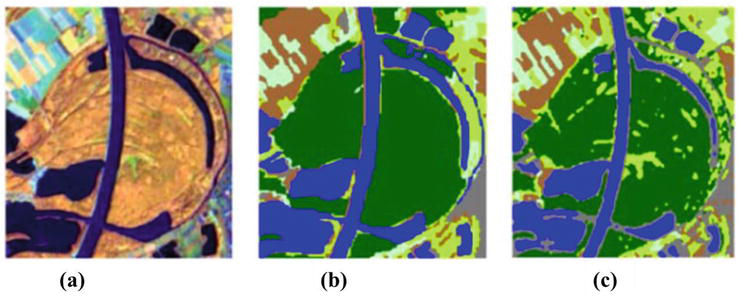
Distinct from pixel-based and sub-pixel-based methods, object-based classification offers a novel paradigm for analyzing remote-sensing imagery [1]. Rather than viewing individual pixels as the elemental units for classification, this approach concentrates on geographical objects—formed through image segmentation [15]—as the foundational units. This methodology is especially advantageous for very high-resolution (VHR) remote-sensing images. Object-based classification integrates spectral, spatial, and contextual information through segmentation techniques, producing more comprehensive image objects for analysis. The central assumption driving this approach is that geographical objects consist of multiple components within an image, thereby enabling a more intricate and accurate representation of complex scenes. Empirical evidence consistently indicates that object-based methods yield substantially higher accuracy rates compared to pixel-based alternatives (Figure 4) [17].

Figure 4.

(a) Satellite image, (b) object-based classification of a satellite image and (c) pixel-based classification of a satellite image [16].

1.2.3 Hybrid classification

The object-based classification approach blends aspects of both manual and automated methods to forge a hybrid system. Analysts can guide the classification process by offering initial input, refining interim results, or injecting domain-specific expertise. At the same time, machine-learning algorithms can be integrated to automate segments of the classification process, enhancing efficiency. This hybrid methodology proves especially beneficial in contexts where the nuanced interpretation provided by human expertise is invaluable, but the speed and scalability offered by automation are also key. Consequently, it is frequently utilized in situations where a mix of manual and automated tactics delivers the best results.

2. Satellite image classification methods

Satellite image classification methods serve as indispensable tools for extracting valuable insights from satellite imagery. They enable the categorization of various features, including land cover and land use, within these images. This section outlines the latest advancements in satellite image classification techniques:

2.1 K-means

K-means clustering, a well-known iterative technique originating from data mining, falls under the category of unsupervised classification known as cluster analysis [18]. In this approach, a set of n observations is divided into k clusters. Each observation is allocated to the cluster to which its mean is the closest. The process starts with the assignment of a random initial cluster vector. Following this, each pixel is classified into the cluster closest to it in terms of distance. The cluster means are then recalculated based on all the pixels contained within each cluster. These latter two steps are repeated until the mean values of the clusters remain stable, effectively minimizing within-cluster variability and leading to cluster convergence. The Sum of Squares Distances function, expressed in Eq. (1), quantifies the relationship between each pixel in the dataset and the centroid (mean) of its designated cluster. This function calculates the squared Euclidean distance between each pixel and the cluster center to which it belongs. This measure is instrumental in determining how closely or loosely each pixel aligns with its cluster centroid, thus shedding light on the level of homogeneity within the clusters as well as the overall efficiency of the clustering process. The ultimate aim of clustering algorithms like K-means is to minimize this Sum of Squares Distances function. By doing so, the algorithm ensures that pixels within the same cluster are as similar as possible while maximizing dissimilarity between distinct clusters. Achieving this goal results in the formation of compact and well-separated clusters, thereby improving the quality of the unsupervised classification outcomes.

$${\mathrm{SS}}_{\text{dist}}={\sum }_{\forall x}{\left[x-c\left(x\right)\right]}^{\mathit{2}}$$E1

where c(x) is the mean of the cluster pixel to which x is assigned.

Minimizing the Mean Squared Error (MSE) is closely linked to minimizing the Sum of Squares Distances (SSdist), as denoted in Eq. (2). The MSE serves as a significant metric for assessing the variability within clusters. It calculates the average of the squared differences between the position of each pixel and the centroid of the cluster to which it belongs. In the context of clustering, a lower MSE value suggests that the pixels within each cluster are tightly grouped around their respective centroids, indicating lower variability and higher internal cohesion. Thus, by aiming to minimize the MSE, one also effectively contributes to the reduction of the SSdist. Achieving this dual minimization helps in creating more compact and well-defined clusters, fulfilling a fundamental goal in both cluster analysis and unsupervised classification methods. This approach enhances the quality of the unsupervised classification output by ensuring that pixels within the same cluster are as similar as possible, thereby also maximizing the dissimilarity between different clusters.

$$\mathrm{MSE}=\frac{{\sum }_{\forall x}{\left[x-C\left(x\right)\right]}^{\mathit{2}}}{{\left(N-c\right)}^b}=\frac{\text{SSdist}}{{\left(N-c\right)}^b}$$E2

2.2 Iterative self organizing data (ISODATA)

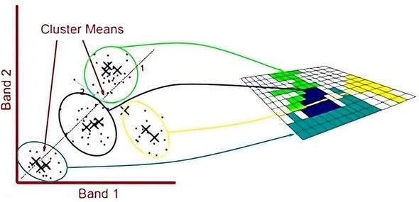
As outlined by [19], the ISODATA algorithm is equipped with a dynamic adjustment mechanism that continually refines the cluster set through a series of iterative calculations. This fine-tuning is achieved primarily through two key processes: cluster assimilation and cluster splitting, visualized in Figure 5. Cluster assimilation is activated under specific conditions: either when the number of pixels within a cluster falls below a predetermined minimum threshold or when the distance between the centroids of two clusters is less than a specified value. In such cases, the algorithm opts to merge or “assimilate” the clusters into a unified group. On the other hand, cluster splitting is initiated when a cluster’s internal standard deviation exceeds a set threshold and when the number of pixels within that cluster is at least double the predetermined minimum. Under these conditions, the algorithm divides or “splits” the existing cluster into two or more separate clusters. These dynamic operations enable the ISODATA algorithm to adjust responsively to the intrinsic variability and complexity present within the dataset. Such adaptability ensures that the resulting clusters are a reliable and precise reflection of the inherent patterns and structures in the data, thereby enhancing the quality of the classification.

Figure 5.

ISODATA classification pixels using cluster means [16].

The ISODATA algorithm stands out for its adaptability in managing datasets that feature a variable number of clusters. Unlike some other clustering algorithms that require a pre-specified number of clusters, ISODATA dynamically adjusts this number during the clustering process. It does so based on the specific traits of the data and the guidelines set for cluster assimilation and splitting, as previously discussed [20]. This feature adds an extra layer of flexibility, making the algorithm well-suited for handling complex datasets where the optimal number of clusters is not easily determinable beforehand.

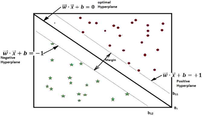
2.3 Support Vector Machine (SVM)

As outlined by [21], the Support Vector Machine (SVM) is grounded in statistical learning theory and is primarily used for classification tasks. It works by partitioning the data into separate classes through a hyperplane designed to maximize the gap, or margin, between these classes. In this context, data points that lie close to the hyperplane are identified as “support vectors,” as illustrated in Figure 6. SVM aims to optimize this margin to reduce the probability of misclassification errors [18]. In achieving this goal, SVM establishes a distinct and unambiguous boundary separating various classes in the dataset.

Figure 6.

Margin of decision boundary in binary SVM classifier [16].

A Binary classification of N training samples and for each instance, consisting of a tuple (x_i, y_i) (i = 1, 2, …, N) where, x i = (x_i1, x_i2, …, x_id) T deals with the attribute set for the ith sample $\in \left\{-\mathit{1},+\mathit{1}\right\}$, and let y_i denote the class labels.

The decision boundary of a linear classifier, in the context of Support Vector Machines (SVM), can be mathematically expressed as:

$$\overrightarrow{\mathrm{W}}\cdot \overrightarrow{\mathrm{X}}+\mathrm{b}=0$$E3

In a binary classification scenario, as is commonly used with Support Vector Machines (SVM), distinct types of data points are given specific class labels for training purposes. For example, if circles are assigned a class label of +1 + 1 and stars are given a class label of −1 − 1, this labeling forms the basis for the classification algorithm. In this context, the class label y for a test sample t can be determined using the following decision rule:

$$\mathrm{y}=\left\{\begin{array}{cc}+\mathit{1}& \text{if}\overrightarrow{W}\cdot \overrightarrow{t}+b>\mathit{0};\\ -\mathit{1}& \text{if}\overrightarrow{W}\cdot \overrightarrow{t}+b<\mathit{0}.\end{array}\right.$$E4

The distance between these two hyperplanes gives the marginal decision boundary (d) (see Eq. (5))

$$\mathrm{d}=\frac{\mathit{2}}{\Vert w\Vert }$$E5

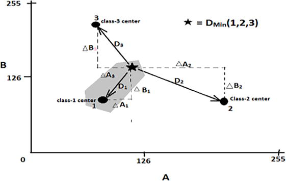
2.4 Minimum Distance Classification

In the Minimum Distance to Means (MDTM) technique, which is a form of supervised classification, a single mean vector that captures its essential spectral characteristics represents each class. For any given pixel in the image, its measurement vector is compared to the mean vectors of each class to calculate spectral distances. Based on these distances, a decision rule, as depicted in Figure 7, is then applied to classify the pixel into one of the predefined classes. The strength of the MDTM classifier lies in its simplicity and computational efficiency, especially when a singular mean vector can adequately represent each class. By directly calculating the spectral distance between a candidate pixel and the mean vectors of each class, the MDTM method ensures that the pixel is classified into the category to which it is most spectrally similar. This approach is particularly useful in scenarios where computational resources are limited but a reasonable level of classification accuracy is still required.

Figure 7.

Calculation of minimum distance between centers of three classes and candidate pixel concerning bands A & B [16].

As specified by Eq. (6), the classifier uses Euclidean distance as the means to calculate the gap between a candidate pixel’s measurement vector and the mean vector of each predefined class. After performing this calculation, the candidate pixel is allocated to the class with the smallest Euclidean distance. This approach leverages the Euclidean distance as a numerical metric for determining the class most spectrally akin to each candidate pixel. By aiming to minimize this distance, the algorithm accurately places the candidate pixel into its most probable class, thereby improving the overall precision of the classification.

$${\mathrm{D}}_{\mathrm{ab}}=\sum _{i=\mathit{0}}^n{\left({\left({\mathrm{a}}_{\mathrm{i}}-{\mathrm{b}}_{\mathrm{i}}\right)}^2\right)}^{1/2}$$E6

where D_ab = distance between class a and pixel b, a_i = mean spectral value of class a in band i, b_i = spectral value of pixel b in band i, and n = number of spectral bands.

2.5 Mahalanobis Distance classifier

As highlighted by [13], the Mahalanobis Distance classifier shares similarities with the Minimum Distance to Means technique, but it adds a key element: the use of a covariance matrix in the classification of satellite images. This matrix captures the statistical interrelationships among various spectral bands, providing a more nuanced and multidimensional metric for measuring the distance between data points than the Euclidean distance used in the Minimum Distance approach. Importantly, the integration of the covariance matrix renders the Mahalanobis Distance classifier particularly effective in situations where the intra-class data distribution exhibits variable levels of variance across different dimensions. As a result, the classifier is more adept at handling the complex spectral interdependencies present in the data, thereby improving the overall accuracy and dependability of the classification.

$$\text{Mahalanobis Distance}\left(\mathrm{Dx}\right)=\frac{{\left(\mathrm{x}-{\mathrm{\mu }}_{\mathrm{i}}\right)}^{\mathrm{T}}}{{\sum }_{\mathrm{i}}}\left(\mathrm{X}-{\mathrm{\mu }}_{\mathrm{i}}\right)$$E7

Where, ∑== pixel covariance matrix for class i, (i = 1,2,........n), μ = average vector of class i

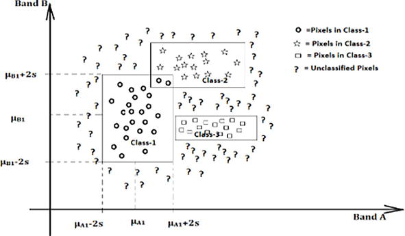
2.6 Parallel Piped classification

As explained by [15], the Parallel Piped classifier divides each axis of the multispectral attribute space into specific regions, often called classes. The limits of these regions are set by the lowest and highest pixel values along each corresponding axis. The success of this classifier in terms of precision and effectiveness largely depends on a thorough analysis of the range for each class, guided by relevant population statistics (as shown in Figure 8). By carefully assessing these ranges, the Parallel Piped classifier strives to accurately allocate pixels to their appropriate classes, thus improving the overall quality and trustworthiness of the image classification process.

Figure 8.

Classification of pixel data based on lowest (μ_A1 − 2s), highest (μ_A1 + 2s), and mean (μ_A1) values on band a and lowest (μ_B1 − 2s), highest (μ_B1 + 2s) and mean (μ_B1) values on band B of class-1 using Parallel Piped approach [16].

In a 2D feature space, the Parallel Piped classifier creates a set of rectangular boxes, each signifying a unique class. Pixels that fall within a particular box are then classified as members of the associated class. This technique is notable for its computational simplicity, as it speeds up the classification process by concentrating on predefined ranges for each class. However, a significant drawback is the possibility of overlapping boxes, which can introduce ambiguity in class assignment. These overlaps occur when the pre-established ranges for various classes intersect, making it challenging to definitively assign pixels in these overlapping areas to a single, distinct class.

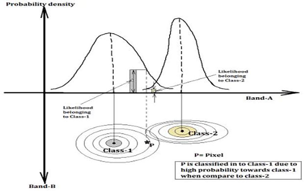
2.7 Maximum Likelihood classification (MLC)

The Maximum Likelihood Classifier (MLC), also known as the Bayesian classifier, is a statistical approach used in supervised classification, as detailed in source [11]. This method classifies pixels into specific classes based on the maximum likelihood estimate that the pixels belong to those classes. The likelihood L_k of a pixel belonging to a particular class k is computed using its posterior probability, as expressed in Eq. (8). The primary goal of this technique is to find the class that maximizes this likelihood, effectively determining the most probable class for the given pixel. Due to its effectiveness in making class assignments grounded in probabilistic logic, the MLC is widely used in the field of remote sensing and various classification tasks.

$${\mathrm{L}}_{\mathrm{k}}=\frac{P\left(k\right)\ast P\left(\frac{K}{x}\right)}{P\left(i\right)\ast P\left(\frac{K}{i}\right)}$$E8

where, P(k) = prior probability of class k, P(k/x) = conditional probability or probability density function of class K.

P(k) and P(i)*P(k/i) are common to all classes. So, L_k depends on the probability density function (Figure 9).

Figure 9.

Concept of Maximum Likelihood classification based on the probability density concerning each class [16].

As demonstrated in Eq. (9), the probability density function (PDF) plays a pivotal role in computing the likelihood of a normal distribution, and its expression is presented as follows [17]. This function serves as a mathematical representation of the probability distribution of data points within a normal distribution, enabling the estimation of the likelihood associated with a specific observation’s membership in this distribution.

$${\mathrm{L}}_{\mathrm{k}}\left(\mathrm{X}\right)=\frac{\mathit{1}}{\sqrt{{\left(\mathit{2}\pi \right)}^{\mathrm{n}}{\gamma }_k}}{\mathrm{e}}^{\frac{-{\left(\mathrm{X}-{\mathrm{x}}_{\mathrm{k}}\right)}^2}{{\mathit{2}}^{\ast }{{\gamma }_k}^2}}$$E9

L_k (X) = likelihood of pixel X belonging to class, k, n = number of satellite image bands, and γ_k = variance-covariance matrix of class k.

2.8 K-Nearest Neighbor Classifier

As elucidated by [14], K-Nearest Neighbors (KNN) is a classification method that primarily relies on majority voting. The algorithm assesses similarity by computing the Euclidean distance between data points in the feature space, as depicted in Eq. (10). KNN employs a predefined parameter, K, to specify the number of nearest neighbors considered in the voting process. Unlike many other classifiers, KNN does not require a specialized training phase. It accomplishes classification by assigning a given data point to the most frequently occurring class among its K-nearest neighbors. This inherent simplicity renders KNN particularly valuable in scenarios where the training dataset may be subject to updates or expansions.

$$\begin{array}{l}\mathrm{Let}\left(\mathrm{x},\mathrm{y}\right)\in \mathrm{D}‐‐>\text{Setoftrainingexamples}\\ \mathrm{k}‐‐>\text{Number of nearest neighbors}\\ \mathrm{z}=\left({\mathrm{x}}^{\prime },{\mathrm{y}}^{\prime }\right)‐‐>\text{Test example}\\ \text{Euclidean Distance}\mathrm{d}\left({\mathrm{x}}^{\prime },\mathrm{x}\right)=\sum _{\mathrm{k}=\mathit{0}}^n{\left({\left({\mathrm{x}}_{\mathrm{k}}^{\prime }-{\mathrm{x}}_{\mathrm{k}}\right)}^2\right)}^{1/2}\end{array}$$E10

In the K-Nearest Neighbors (KNN) algorithm, the classification of a test example is accomplished by identifying its K-nearest neighbors within the feature space, a calculation delineated by the method outlined in Eq. (11). Once the nearest neighbors are determined, the test example is assigned a label based on the majority class within this neighbor list. The underlying principle guiding this approach is that of spatial proximity: the class that appears most frequently among the closest neighbors of the test example is considered the most probable class for the test example itself. This technique harnesses the strength of local information to make global predictions.

$$\begin{array}{l}\text{Majority voting}:{\mathrm{y}}^{\prime }=\text{argmax}{\sum }_{\left(x_i,y_i\right)\in D_z}I\left(v=y_i\right)\\ \mathit{\text{Where}},v‐‐>\mathit{\text{class}}\mathit{\text{label}}\\ y_i‐‐>\mathit{\text{Class}}\mathit{\text{label}}\mathit{\text{for}}\mathit{one}\mathit{\text{of}}\mathit{\text{the}}\mathit{\text{nearest}}\mathit{\text{neighbors}}.\end{array}$$E11

In certain scenarios, the K-Nearest Neighbors (KNN) classifier may encounter challenges when classifying certain test records. Such situations arise when the test records bear limited resemblance to or have little correspondence with the training instances. As KNN heavily relies on the proximity of test records to training data points, if there are no nearby neighbors from the training set within the specified value of K, the classifier may struggle to make confident classifications. This issue is particularly pronounced when dealing with sparse or high-dimensional datasets, where accurately defining the distances between data points becomes a complex task. To address this challenge, various techniques can be employed, including data preprocessing, feature selection, or dimensionality reduction, to enhance the performance of the KNN classifier and bolster its ability to effectively classify diverse test records.

2.9 Artificial Neural Networks (ANN)

Artificial Neural Networks (ANNs) constitute a specialized subset of artificial intelligence designed to emulate certain aspects of the human brain, particularly the capability to assign meaningful labels to individual pixels in images. ANNs employ a nonparametric classification approach and possess inherent adaptability, allowing for the integration of additional data to enhance accuracy, as demonstrated in prior research [5]. Structurally, an ANN is organized into multiple layers, each containing neurons, which are processing units. These neurons are interconnected through weighted connections spanning across adjacent layers. During the training phase, ANNs analyze patterns within the training data to derive actionable insights. These insights aid in the formulation of generalizable rules that can be applied to classify previously unseen data, aligning with the foundational principles proposed by [22]. ANNs prove highly effective in addressing complex classification challenges, consistently outperforming more methods that are rudimentary. Numerous ANN algorithms are specifically tailored for classifying remotely sensed images, including but not limited to:

2.9.1 Multi-layer perceptron (MLP)

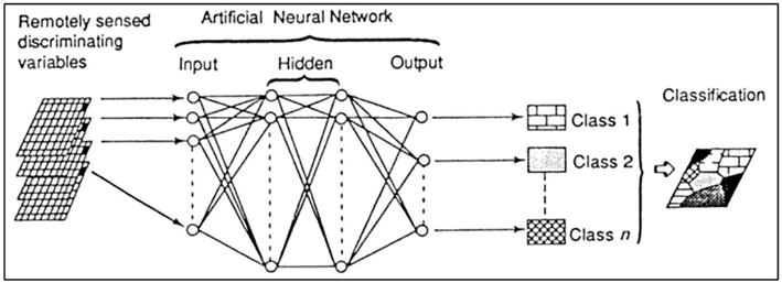
The Multi-layer perceptron (MLP) represents one of the most widely utilized subtypes of Artificial Neural Networks (ANNs). Operating as a feed-forward ANN model, the MLP is designed to establish mappings between sets of input data and their respective outputs, a concept that was initially introduced in prior research [23]. Structurally, the MLP comprises three essential layers: an input layer, an output layer, and one or more hidden layers. These layers are interconnected sequentially, as depicted in Figure 2. Users enjoy the flexibility to determine the number of neurons allocated to each layer. Specifically, the neurons in the input layer represent the input variables, while those in the output layer correspond to the categories defined by the training data. Typically, each input variable is mapped to a single neuron in the input layer, and each class of interest is associated with its own neuron in the output layer. The training process of the MLP employs a supervised learning algorithm commonly known as back-propagation. The mathematical formalism for this process can be expressed as follows:

$$y=\phi \left(\sum _{i=1}^n{w}_i{x}_i+b\right)=\phi \left(w^{T}x+b\right)$$E12

where:

• W = represents the vector of weights.

• x = is the vector of inputs.

• b = stands for the bias.

• φ = denotes the activation function, typically chosen as the sigmoid function, which is expressed as 1/(1 + e-x). As demonstrated by [24], this particular activation function has proven effective in modeling nonlinear mappings.

In the framework of MLP, the weights and activation functions serve as critical elements within the neurons. During the training phase, neurons in both the input and hidden layers are initialized with random weights. Each pixel in the training data is then mapped to a likelihood of activating a specific output neuron, based on its maximum activation value. Subsequent solutions are evaluated in comparison, with the solution yielding the lowest error being retained. This iterative procedure persists until the network achieves an acceptable level of testing error for mapping input variables to the predetermined output classes. Once the network is adequately trained, it is deployed to classify the remaining dataset according to the activation level demonstrated by individual pixels, following the methodology described in [25]. However, one significant challenge associated with MLP is the necessity to retrain the entire network for any required adjustments. Such retraining could alter or nullify previously learned information, thereby prolonging the training duration—even when dealing with relatively modest datasets, as observed by [26]. To augment the efficiency of MLP classifiers without a corresponding substantial increase in computational time [22, 27], researchers have suggested specific parameter values, which are summarized in Table 1. Here, “N” denotes the number of classes (Figure 10).

Number of hidden layers/nodes	Between 2Ni to 3Ni
Learning rate	0.01–0.001
Momentum factor	0.5
Sigmoid constant	1
RMSE	0.0001
Number of iterations	10,000
Accuracy rate percent	100%

Table 1.

The basic architecture to start MLP [28].

Figure 10.

A typical MLP with back-propagation [22] reported by [28].

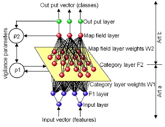
2.9.2 Fuzzy ArtMap classification

Fuzzy ArtMap is a classification technique rooted in Adaptive Resonance Theory (ART), as originally introduced by [29]. This approach employs a clustering methodology designed for vectors with fuzzy inputs, which are represented as real numbers within the range of 0 to 1. Fuzzy ArtMap incorporates an incremental learning mechanism, allowing for continuous learning while preserving previously acquired knowledge, as elaborated upon by [30]. A distinctive feature of Fuzzy ArtMap is its emphasis on retaining only the weights of neurons encoding the class that best matches the input pattern. This characteristic enables it to effectively handle large-scale problems with relatively few training epochs. However, Fuzzy ArtMap is susceptible to noise and outliers, which can lead to an increased number of misclassified data points. The Fuzzy ArtMap architecture consists of four layers of neurons: the input layer (F1), category layer (F2), map field, and output layer. To configure Fuzzy ArtMap effectively, five key parameters must be specified, as outlined in Table 2 by [31]:

Choice parameter α	A small positive constant
Learning rate parameters β1 in ARTa	0 ≤ β1 ≤ 1
Learning rate parameters β2 in ARTb	0 ≤ β2 ≤ 1
Vigilance parameters ρ1 in ARTa	Normally set very close to 1
Vigilance parameters ρ2 in ARTb	Normally set very close to 1

Table 2.

The proposed parameters to start Fuzzy ArtMap [28].

The parameters ρ1 and ρ2 play a pivotal role in both the learning and operational phases of the network, exerting significant influence over the entire process. During the learning phase, the weights of neurons in both the map field and the category layer undergo dynamic adaptation. This adaptability is driven by the spectral characteristics inherent to each observed input pixel in the first input layer (F1). The assignment of an observation from the input layer (F1) to a neuron in the category layer (F2) hinges on the spectral features of the given observation. In instances where none of the existing neurons in F2 satisfies the predefined similarity threshold criteria for a particular observation in F1, a new F2 neuron is created. The generation of new neurons in F2 effectively partitions the dataset into subsets characterized by a user-specified degree of homogeneity (Figure 11). This degree of homogeneity is governed by a “vigilance parameter,” originally conceptualized by [15].

Figure 11.

Fuzzy ArtMap architecture [32] reported by [28].

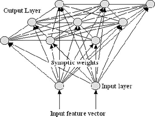
2.9.3 Self-Organized Feature Map (SOM)

SOM, initially proposed by [33], features a single-layer neural network architecture, as depicted in Figure 4. In this setup, the input layer corresponds to the feature vector, with individual neurons representing separate measurement dimensions. According to guidelines from [34], a typical output layer in an SOM is arranged as a 15 x 15 neuron grid. Arrays smaller than this may compromise the granularity needed for distinct class representation, while larger arrays generally improve classification accuracy. The synaptic weights linking the neurons of the output layer to the input layer neurons are initially randomized. These weights are subsequently reorganized through iterative sampling of the input data. This adjustment process leads to the spatial clustering of neurons with similar synaptic weights, as shown in Figure 12. During the training phase, neurons close to the ‘winning’ neuron—determined by the closeness between the input vector and its synaptic weight, as described in [35]—are actively engaged in learning. In this context, X = (x1, x2, x3, …, xn) signifies the SOM’s reflectance vector for a single pixel input. The training process consists of two primary stages:

1. Unsupervised classification phase: neuron weights are regionally structured through competitive learning and lateral interactions, thereby establishing the network’s topology.

2. Refinement phase: the decision boundaries delineating various classes are further refined by integrating training samples via the Learning Vector Quantization (LVQ) algorithm, as elaborated by [36].

Figure 12.

Example of an SOM with a two-neuron input layer and 3 × 3-neuron output layer [28].

In the classification step, each pixel is assigned a class based on the neuron or neurons with weight vectors most similar (in terms of minimal Euclidean distance) to the pixel’s reflectance vector. Unlike other architectures like MLP or Fuzzy ArtMap, SOM takes into account inter-class relationships, facilitating the classification of multimodal classes. A notable drawback, however, is the occasional emergence of unclassified pixels, as highlighted by [37]. To optimize classification accuracy without substantially increasing computational load, recommended parameter settings for SOM classifiers are presented in Table 3.

Course tuning parameters				Fine-tuning parameters
Output neurons	Initial	Min.	Max.	Min.	Max.	Fine-tuning
	γ	α	α	δ^t	δ^t	epoch
225 (15 × 15)	25	0.5	1	0.0001	0.0005	50

Table 3.

The proposed parameters to start SOM [28].

2.9.4 Radial Basis Function Network (RBFN)

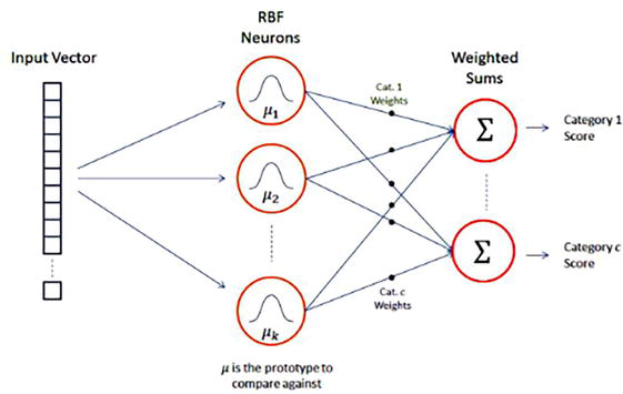
The Radial Basis Function Network (RBFN) is a type of nonlinear neural network designed for classification tasks. This network architecture consists of three primary layers: an n-dimensional input vector, a hidden layer of Radial Basis Function (RBF) neurons, and an output layer with individual nodes corresponding to each data category or class. The central aim of an RBFN is to classify data by evaluating the similarity between incoming inputs and stored prototypes within the RBF layer. Each neuron in the RBF layer contains a prototype, which is essentially a representative example from the training dataset. A commonly used method for selecting these prototypes involves applying k-means clustering to the training data, with the resultant cluster centers serving as the prototypes. During the network’s operation, each RBF neuron calculates the Euclidean distance between its stored prototype and the incoming input vector. This distance is then converted into an activation value that falls between 0 and 1, serving as an indicator of similarity. In this context, an activation value of 1 signifies a perfect match between the input and the prototype, while the activation value decreases exponentially toward zero as the distance between the input and the prototype grows. The output layer’s nodes then compute a score for each potential data category. This score is obtained through a weighted sum of the activation values generated by the RBF neurons in the hidden layer. Before contributing to the final score, each neuron’s activation is multiplied by its corresponding weight. The final classification decision is usually made by allocating the input to the category associated with the highest computed score (Figure 13).

Figure 13.

RBF network architecture [28].

Various similarity functions can be employed in the context of Radial Basis Function Networks (RBFNs), among which the Gaussian function is often favored, particularly for one-dimensional data. For instance, Eq. (13) outlines the form of a typical Gaussian function where ‘x’ is the input, ‘μ’ represents the mean, and ‘σ’ stands for the standard deviation. Notably, the activation function for an RBF neuron does exhibit slight variations, as shown in Eq. (14). The training regimen for an RBFN requires the optimization of three key parameter sets: the prototypes (μ), the β coefficients associated with each RBF neuron, and the output weight matrix connecting the RBF neurons to the nodes in the output layer. To improve classification accuracy, [38] suggests setting the μ and β parameters at specific values, namely 1.05 and 5, respectively.

$$f\left(x\right)=\frac{1}{\sigma \sqrt{2\pi }}{e}^{-\frac{{\left(x-\mu \right)}^2}{2{\sigma }^2}}$$E13

$$\phi \left(x\right)=e^{-\beta {‖x-\mu ‖}^2}$$E14

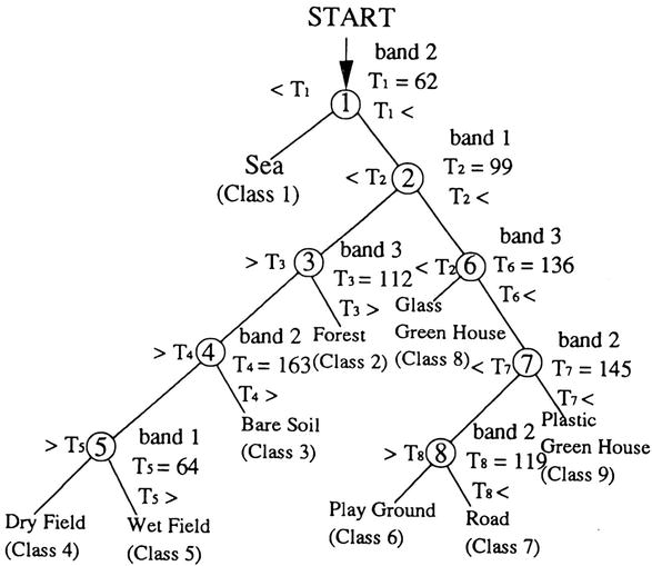
2.10 Classification Trees (CTs)

Classification Trees (CTs) were originally conceptualized by [39] as a non-parametric, iterative, and hierarchical approach to pattern recognition. A Classification Tree consists of multiple essential components: a root node, which serves as the starting point; non-terminal nodes, which are positioned between the root and terminal nodes; and terminal nodes, which group pixels belonging to the same class, as illustrated in Figure 14. One of the key strengths of CTs is their capacity to recursively divide a dataset into increasingly homogeneous subsets, employing binary splitting rules as elaborated by [15]. These splitting rules are informed by the training data and are based on statistical techniques, with the metric of ‘impurity’ playing a crucial role. A node is considered ‘pure’ when it contains pixels exclusively from a single category, leading to an impurity score of zero. As the algorithm traverses the tree, it evaluates a logical condition at each node. Depending on the outcome of this evaluation, it moves to either the left or the right child node. This iterative partitioning persists until a node reaches a state of purity, at which point it is labeled as a terminal node.

Figure 14.

Classification tree. The numbers indicate the variables and their values as thresholds for each node condition [28].

The key splitting rules commonly used in Classification Trees (CTs) include:

1. Entropy: originated by [40], this measure assesses node homogeneity and aims to minimize entropy, ideally driving it to zero for a pure terminal node.

2. Information Gain (IG) or Gain ratio: further developed by [41], IG calculates the entropy reduction resulting from splitting a node N according to rule T. The attribute offering the highest IG is chosen for the split. One limitation is its bias toward variables with greater variances, which may lead to excessive splitting. This is often mitigated by normalizing the Information Gain with respect to the entropy of the created partitions.

3. Gini index: based on methods described by [39], this index measures node impurity and aims to find the most homogenous subsets within the training data. The rule that maximizes impurity reduction—or equivalently minimizes the Gini index—is selected for the split.

The potential for overfitting exists when a CT becomes too tailored to the training data, capturing noise that may affect its generalization capability. Pruning strategies are employed to counter this, often reducing the tree size by up to 25% and enhancing its predictive performance. Among the pruning methods, 10-fold cross-validation has gained recognition for its robustness, necessitating an independent dataset for performance assessment. Typically, pruned trees deliver the best classification accuracy. For a more comprehensive understanding of cross-validation, see [42].

2.11 Fuzzy classifiers

Fuzzy classifiers quantify the degree of fuzzy set membership for each pixel concerning specific classes. This degree is determined by calculating the standardized Euclidean distance from the mean of the class signature through a particular algorithm. In essence, the mean of a class signature symbolizes the optimal point for that class, where fuzzy set membership attains its maximum value of 1. As the distance from this point increases, the membership value diminishes, reaching zero at a user-defined distance threshold. Among the myriad fuzzy classification algorithms, Fuzzy C-Means (FCM) stands out for its effectiveness, especially in tasks involving overlapping clusters. Initially introduced by [43], FCM aims to minimize a fuzzy objective function, denoted as J_m, in an iterative optimization process, as illustrated in Eq. (15).

$$J_m=\sum _{i=1}^c\sum _{k=1}^n{\left({\mu }_{\mathit{ik}}\right)}^m{d}^2\left(x_k,V_i\right)$$E15

where:

• c = number of clusters

• n = total pixel count

• μik = membership value for the i-th cluster of the k-th pixel

• m = fuzziness factor for each fuzzy membership

• xk = vector representing the k-th pixel

• Vi = centroid vector of the i-th cluster

• 2d2(xk,Vi) = squared Euclidean distance between xk and Vi

The membership (μik) is calculated by measuring the distance between the k-th pixel’s vector and the centroid of the i-th cluster. These calculated membership values are subject to the following constraints:

$$\left\{\begin{array}{l}0\le {\mu }_{\mathit{ik}}\le 1\text{for}\mathrm{all}i,k\\ \sum _{i=1}^c{\mu }_{\mathit{ik}}=1\text{for}\mathrm{all}k\\ 0<\sum _{k=1}^n{\mu }_{\mathit{ik}}<n\text{for}\mathrm{all}i\end{array}\right.$$E16

The cluster center (Vi) and the membership value (μik) can be calculated using Eqs. (17) and (18), respectively.

$$V_i=\frac{{\sum }_{k=1}^n{\left({\mu }_{\mathit{ik}}\right)}^m{x}_k}{{\sum }_{k=1}^n{\left({\mu }_{\mathit{ik}}\right)}^m},1\le i\le c$$E17

$$\begin{array}{l}{\mu }_{\mathit{ik}}={\left[\sum _{j=1}^c{\left(\frac{d\left(x_k,V_i\right)}{d\left(x_k,V_j\right)}\right)}^{\frac{2}{m-1}}\right]}^{-1},1\le i\le \\ c,1\le k\le n\end{array}$$E18

To minimize J_m, a repetitive procedure is followed, governed by Eqs. (17) and (18). The process begins by establishing fixed values for c (the number of clusters), the degree of fuzziness m, and a convergence tolerance ϵ, in addition to initializing the starting centers for each cluster. Subsequently, the values of μik and Vi are computed in accordance with Eqs. (17) and (18). The iterative process continues until the variation in Vi between two consecutive iterations falls below the specified threshold ϵ. Eventually, each pixel is assigned a category based on its varying degrees of membership across multiple clusters.

3. Hybrid Classifiers

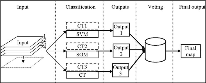
Different classifiers often yield varying class assignments when applied to the same test area, highlighting the fact that no single classifier can deliver optimal performance across all classes. Various classification algorithms exhibit complementary characteristics, as supported by the research presented in [44]. Neural and statistical algorithms, in particular, demonstrate such complementary behavior. These classifiers tend to produce uncorrelated classification errors, which in turn facilitate the attainment of improved classification accuracies when they are combined. In the context of a hybrid classifier-based approach, it is crucial for the individual classifiers to either employ independent sets of features or be trained on distinct training datasets. Essentially, there are two primary strategies for combining classifiers:

1. Classifier ensembles (CE).

2. Multiple classifier systems (MCS), as illustrated in Figure 15.

Figure 15.

Classifier ensemble (dashed) versus multiple classifier systems (solid) [28].

In situations where the classification outcomes from multiple classifiers demonstrate a high degree of similarity, the amalgamation of these classifiers may only sporadically yield improvements in classification accuracy. This underscores the pivotal importance of classifier diversity for the effective implementation of hybrid systems, a point emphasized by the findings reported in [45]. Although not frequently employed or scrutinized in the context of remote-sensing image classification, measures of classifier diversity are indispensable for evaluating the variations among different algorithms. Such metrics encompass Kappa statistics [46], the double fault measure [47], agreement measures [48], similarity indices, measures of non-inferiority and difference [49], weighted counts of errors and correct results (WCEC) [50], entropy-based metrics [51], and the Disagreement-accuracy measure [52].

4. Comparison of satellite image classification methods

Numerous studies have been undertaken to compare unsupervised, supervised, and hybrid methods for satellite image classification, focusing on evaluation criteria such as classification accuracy and various alphanumeric constants. This section offers a comprehensive review of these comparative analyses. Table 4 delineates the merits and demerits of conventional classifiers, as cited in [53], while Table 5 engages in a more detailed discussion concerning the advantages and disadvantages inherent to various classification approaches. The task of selecting the most apt classifier for a given dataset poses a significant challenge, chiefly due to the absence of straightforward guidelines to facilitate this decision-making process. Furthermore, the image classification workflow involves a series of decisions and choices that must be made by the analyst. To elucidate the comparative strengths and limitations of unsupervised, supervised, and hybrid techniques, extensive comparative studies have been conducted. Table 6 synthesizes findings from various researchers concerning the efficacy of different classifiers and the contexts in which they are most effective. It is noteworthy that there exists no universal agreement among researchers as to which classification methodology is unequivocally superior. As a result, the choice of an appropriate classifier is often contingent upon the specific requirements and objectives of the project at hand.

Classifier	Advantages	Disadvantages
ISODATA	Fast and simple to process	Needs several parameters
K-means	Fast and simple to process	Could be influenced by: the number and position of the initial cluster centers specified by the analyst, the geometric properties of the data, and clustering parameters
KNN	Simple to process	Computationally expensive when the training dataset is large
MD	Fast and simple to process	Considers only mean value
MhD	Fast and simple to process	Considers only mean value
PP	Fast and simple to process	Overlap may reduce the accuracy of the results
MXL	Sub-pixel classifier	Time consuming Insufficient ground truth data and/or correlated bands can affect the results Cannot be applied when the dataset is not normally distributed

Table 4.

Comparison of classic classification techniques.

Method	Advantages	Disadvantages
ANN	Non-parametric classifiers High computation rate of very large datasets Efficiently handles noisy inputs	It is difficult to understand how the result was achieved. The training process is slow. Problem of over fitting Difficult to select the type network architecture Dependent on user-defined parameters
CTs	Non-parametric classifiers Does not require an extensive design and training Easy to understand the classification process Accurate, and computational efficiency is good Easy to integrate multi-source data	Calculation becomes complex when various outcomes are correlated.
SVMs	Non-parametric classifiers Provides a good generalization The problem of over fitting is controlled. Computational efficiency is good. Perform well with minimum training set size and high-dimensional data Often outperform other classifiers.	Training is time consuming. Difficult to understand its structure Dependent on user-defined parameters Determination of optimal parameters is not easy.
Fuzzy Classifiers	Efficiently handle overlapping data Minimize computation time and reduce memory requirements	Without priori knowledge output is not good.

Table 5.

Comparison of modern classification techniques [54].

Researcher	Classifier	Datasets	Best performance
Pal and Mather [55]	SVMs MXL ANN	Landsat 7 ETM+ Hyperspectral data	SVMs
Oliveira et al. [30]	MXL CTs MLP SOM ArtMap CTs	Landsat (ETM+)	ArtMap
Lippitt et al. [56]	SOM MLP ArtMap CTs	Landsat 7 (ETM+)	CTs
Li et al. [31]	MXL CTA ArtMap KNN	Landsat 5 TM ALSO PALSAR (L-band HH and HV)	ArtMap
Maryam et al. [57]	SVMs MXL MD PP	Landsat 7 ETM+	SVMs
Shaker et al. [58]	Contextual MXL MD	SPOT	MXL
Mannan et al. [59]	ArtMap MXL MLP	IRS-1B	ArtMap
Gil et al. [60]	SVMs ANN MXL	IKONS	SVMs
Du et al. [52]	MLP ANN CTs MXL SVMs ArtMap	Quick Bird Spectral/textural features	SVMs
Doma et al. [61]	PP MD MXL ANN SVMs	Quick Bird	SVMs
Hamedianfar et al. [62]	OO/fuzzy SVMs	World View-2 (WV-2)	OO/fuzzy
Camps-Valls et al. [63]	SVMs ANN	Hyperspectral data (128 bands)	SVMs
Trinder et al. [64]	SVMs SOM CTs	Aerial images LiDAR data	SVMs
Kanika et al. [65]	ANN MD MLC	IRIS Plants Dataset	ANN
Jamshid et al. [66]	ISODATA MLC HM	Desert Outlay Datasets	HM
Offer and Arnon [67]	MLC MD PP	Landsat 7 ETM+	MLC
Aykut et al. [68]	PP MD CM	Landsat 5 TM	CM
Shila and Ali [69]	Unsupervised Supervised HM	Landsat 7 ETM +	HM
Maryam et al. [57]	SVMs MLC MHD MD SID BCs PP	Landsat 7 ETM +	SVMs
Manoj et al. [14]	KM ISODATA MD MLC PP SRG ESRG	Landsat, SPOT and IRS Datasets	ESRG
Subhash et al. [70]	MLC MD MHD	Landsat 7 ETM +	MLC
Malgorzata et al. [71]	PBC OOC	Multi-spectral Satellite Images	OOC

Table 6.

Performance evaluation of various classification methods against different datasets.

5. Selection and evaluation process of satellite image classification methods

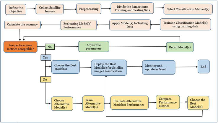
The evaluation process and the selection of methods and techniques for satellite image classification represent a critical phase in any remote-sensing or Earth observation study. This stage involves careful consideration of various factors, including the characteristics of the satellite data, the specific objectives of the classification task, and the computational resources available. Researchers must weigh the strengths and weaknesses of different classification algorithms, such as Artificial Neural Networks, Support Vector Machines, and Classification Trees, in order to make an informed choice. Furthermore, evaluation criteria extend beyond mere accuracy and encompass factors like computational efficiency, ease of implementation, and the ability to handle challenges like overfitting or underfitting. This rigorous process ensures that the selected methods and techniques align with the project’s objectives, providing meaningful insights into the Earth’s dynamics and environmental changes based on satellite imagery, as described in Figure 16.

Figure 16.

Selection and evaluation process of satellite image classification methods and techniques.

This figure provides a comprehensive overview of the systematic process employed in the selection and evaluation of satellite image classification methods and techniques. It guides readers through the intricate steps involved in methodological decision-making, offering a clear depiction of how various algorithms are chosen, assessed, and ultimately applied to satellite image classification tasks. This visual representation enhances the clarity of our research, helping both novice and experienced researchers in the field to grasp the complexity of the decision-making process and its significance in achieving accurate and meaningful results.

6. Summary and discussion

In the classification of remotely sensed images, numerous Artificial Neural Network (ANN) algorithms have been implemented. Multilayer Perceptron (MLP), Self-Organizing Maps (SOM), and Fuzzy ArtMap are some examples. Fuzzy ArtMap has emerged as the most effective, followed closely by MLP. In contrast, SOM has consistently demonstrated the lowest classification accuracy across numerous investigations. Importantly, the performance of these algorithms is extremely dependent on the expertise of the operator in fine-tuning algorithmic parameters. MLP is effective, but it requires a complete reprogramming of the network, which is a disadvantage. This can be a time-consuming operation, particularly for smaller test areas. To mitigate this, pre-trained models could be used as a starting point. Fuzzy ArtMap, on the other hand, is adept at dealing with large-scale problems and requires fewer training iterations. However, it is susceptible to noise and outliers, which may impact classification accuracy negatively. Preprocessing steps to remove noise can help overcome this challenge. SOM, unlike MLP and Fuzzy ArtMap, is capable of distinguishing between multimodal classes but frequently leaves a greater number of pixels unclassified. This can be mitigated by adjusting parameters or using hybrid approaches. Entropy splitting has become the algorithm of preference when it comes to Classification Trees (CTs) for image classification. The 10-fold cross-validation method is also recognized for its dependability and precision. CTs developed for one test area can frequently be successfully transferred to another, provided that the remotely sensed images share similar sensor characteristics and Land Use and Land Cover (LULC) patterns. Support Vector Machines (SVMs) flourish in classification precision and class-specific error balance. The Radial Basis Function (RBF) kernel is frequently the best option among the numerous kernels. However, determining the optimal RBF kernel parameters, specifically C, typically requires a grid search and 10-fold cross-validation. It is essential to recognize that various classifiers provide distinct data perspectives. While some classifiers excel at identifying particular classes, others are better adapted for distinguishing between distinct groups. Consequently, combining classifiers efficiently can result in greater classification accuracy than using a single classifier, even if it is extremely effective. When combined, neural and statistical classifiers frequently generate uncorrelated errors, thereby enhancing the overall classification accuracy. Adding more classifiers does not necessarily enhance performance, though. Diversity is a crucial success factor for hybrid systems. Combinations of classifiers selected based on the Disagreement accuracy metric typically outperform those selected using other diversity metrics. Both Classifier Ensembles (CE) and Multiple Classifier Systems (MCS) are based on aggregating multiple instances of the identical algorithm.

7. Conclusion

In recent decades, significant progress has been made in the field of picture classification, mostly due to the emergence and utilization of sophisticated classification algorithms. This comprehensive review aims to provide invaluable guidance for researchers by dissecting the strengths and limitations of each approach, with special emphasis on their suitability in various contexts. Artificial Neural Networks, particularly Multilayer Perceptrons (MLPs) and Fuzzy ArtMap, present distinct considerations, chiefly revolving around computational complexity and parameter tuning. MLPs often necessitate an extensive network reconfiguration, a time-consuming process, especially for smaller datasets. Nevertheless, their adaptability makes them well-suited for intricate classification tasks. Fuzzy ArtMap excels in managing large-scale problems with fewer training iterations but is sensitive to noise and outliers, demanding meticulous pre-processing for accuracy. In the case of Support Vector Machines, the selection of a kernel function and its associated parameters significantly influence classification outcomes. The Radial Basis Function (RBF) kernel frequently outperforms others in terms of effectiveness, yet pinpointing optimal parameters typically involves computationally intensive grid search and 10-fold cross-validation. SVMs excel at maintaining class-specific error balance but may encounter challenges with excessively large or imbalanced datasets. On the contrary, Classification Trees offer interpretability and ease of use as their primary advantages. They possess the ability to conduct feature selection as an integral part of the model-building process, effectively reducing dimensionality. However, they are susceptible to overfitting, particularly when the tree structure becomes overly complex. Techniques such as pruning and cross-validation can help alleviate this concern. While entropy-based splitting rules have proven effective, the algorithm’s performance may vary depending on the chosen impurity measure. Additionally, this review underscores the vital role of algorithmic optimization, elaborating on the selection and combination of base classifiers to enhance performance. Diversity measures assume a pivotal role in guiding ensemble construction, ensuring more reliable and robust classification results. The review synthesizes these intricate details by drawing upon collective insights from existing studies, enabling researchers to align their methodological preferences with project-specific requirements and constraints. Evaluation criteria encompass not only accuracy but also extend to considerations such as computational cost, ease of implementation, and resilience to overfitting or underfitting, all tailored to the characteristics of each algorithm. This exhaustive study not only aggregates diverse viewpoints but also serves as a pragmatic roadmap for future research endeavors. By comprehensively presenting the advantages and practical challenges associated with each method, along with their specific evaluation criteria, it aims to empower researchers with a nuanced understanding, enabling them to make well-informed decisions within the realm of satellite image classification.

Acknowledgments

This chapter was supported by the project TKP2021-NVA-13 (BorderEye) which has been implemented with the support provided by the Ministry of Culture and Innovation of Hungary from the National Research, Development and Innovation Fund, financed under the TKP2021-NVA funding scheme.

References

1.Jensen JR. Introductory Digital Image Processing: A Remote Sensing Perspective. 3rd ed. Upper Saddle River: Prentice-Hall; 2005
2.Chaichoke V, Supawee P, Tanasak V, Andrew KS. A normalized difference vegetation index (NDVI) time-series of idle agriculture lands: A preliminary study. Engineering Journal. 2011;15(1):9-16
3.Lu D, Weng Q. A survey of image classification methods and techniques for improving classification performance. International Journal of Remote Sensing. 2007;28(5):823-870
4.Kumar S, Kumar D. A review of remotely sensed satellite image classification. International Journal of Electrical and Computer Engineering. 2019;9(3):1720
5.Abburu S, Golla S. Satellite image classification methods and techniques: A review. International Journal of Computer Applications. 2015;119(8):20-25
6.Kulkarni AD, Kamlesh L. Fuzzy neural network models for supervised classification: Multispectral image analysis. Geocarto International. 1999;4:42-51. DOI: 10.1080/10106049908542127
7.Wu C, Murray AT. Estimating impervious surface distribution by spectral mixture analysis. Remote Sensing of Environment. 2003;84:493-505. DOI: 10.1016/S0034-4257(02)00136-0
8.Yang CC, Prasher SO, Enright P, Madramootoo C, Burgess M, Goel PK, et al. Application of decision tree technology for image classification using remote sensing data. Agricultural Systems. 2003;76:1101-1117. DOI: 10.1016/S0308-521X(02)00051-3
9.Blaschke T. Object based image analysis for remote sensing. Journal of Photogrammetry and Remote Sensing (ISPRS). 2009;65:2-16. DOI: 10.1016/j.isprsjprs.2009.06.004
10.Pal NR, Bhandari D. On object background classification. International Journal of Systems Science. 1992;23:1903-1920. DOI: 10.1080/00207729208949429
11.Benz UC, Hofmann P, Willhauck G, Lingenfelder I, Heynen M. Multi-resolution, object-oriented fuzzy analysis of remote sensing data for GIS-ready information. Journal of Photogrammetry and Remote Sensing (ISPRS). 2004;58:239-258. DOI: 10.1016/j.isprsjprs.2003.10.002
12.Ahmed R, Mourad Z, Ahmed BH, Mohamed B. An optimal unsupervised satellite image segmentation approach based on Pearson system and k-means clustering algorithm initialization. International Science Index. 2016;3(11):948-955
13.Al-Ahmadi FS, Hames AS. Comparison of four classification methods to extract land use and land cover from raw satellite images for some remote arid areas, Kingdom of Saudi Arabia. Journal of King Abdul-Aziz University, Earth Sciences. 2009;20(1):167-191
14.Manoj P, Astha B, Potdar MB, Kalubarme MH, Bijendra A. Comparison of various classification techniques for satellite data. International Journal of Scientific & Engineering Research. 2013;4(2):1-6
15.Tso B, Mather PM. Classification Methods for Remotely Sensed Data. 2nd ed. America: Taylor and Francis Group; 2009
16.Rajyalakshmi D, Raju KK, Varma GS. Taxonomy of satellite image and validation using statistical inference. In: 2016 IEEE 6th International Conference on Advanced Computing (IACC). Bhimavaram, India: IEEE; 2016. pp. 352-361
17.Shalaby A, Tateishi R. Remote sensing and GIS for mapping and monitoring land cover and land-use changes in the northwestern coastal zone of Egypt. Applied Geography. 2006;27:28-41. DOI: 10.1016/j.apgeog.2006.09.004
18.Marconcini M, Camps-Valls G, Bruzzone L. A composite semi-supervised SVM for classification of hyperspectral images. IEEE Geoscience and Remote Sensing Letters. 2009;6:234-238. DOI: 10.1109/LGRS.2008.2009324
19.Deer PJ, Eklund P. Study of parameter values for a Mahalanobis distance fuzzy classifier. Fuzzy Sets and Systems. 2003;137:191-213. DOI: 10.1016/S0165-0114(02)00220-8
20.Zhang B, Li S, Jia X, Gao L, Peng M. Adaptive Markov random field approach for classification of hyperspectral imagery. Geoscience and Remote Sensing, IEEE. 2011;8:973-977. DOI: 10.1109/LGRS.2011.2145353
21.Zhu HW, Basir O. An adaptive fuzzy evidential nearest neighbor formulation for classifying remote sensing images. IEEE Transactions on Geoscience and Remote Sensing. 2005;43:1874-1889. DOI: 10.1109/TGRS.2005.848706
22.Foody GM. Image classification with a neural network: From completely crisp to fully-fuzzy situations. In: Atkinson PM, Tate NJ, editors. Advances in Remote Sensing and GIS Analysis. Chichester: Wiley & Son; 1999
23.Rosenblatt F. Principles of Neurodynamics: Perceptrons and the Theory of Brain Mechanisms. Washington DC: Spartan Books; 1962. Available from: http://catalog.hathitrust.org/Record/000203591
24.Cybenko G. Approximation by superpositions of a sigmoidal function. Mathematics of Control, Signals, and Systems. 1989;2(4):303-314
25.Foody GM. Land-cover classification by an artificial neural network with ancillary information. International Journal of Geographical Information Systems. 1995;9(5):527-542
26.Liu W, Seto K, Wu E, Gopal S, Woodcock C. ARTMMAP: A neural network approach to subpixel classification. IEEE Transactions on Geoscience and Remote Sensing. 2004;42(9):1976-1983
27.Kavzoglu T, Mather PM. The use of back-propagating artificial neural networks in land cover classification. International Journal of Remote Sensing. 2003;24(3):4907-4938
28.Salah M. A survey of modern classification techniques in remote sensing for improved image classification. Journal of Geomatics. 2017;11(1):21
29.Carpenter GA, Crossberg S, Reynolds JH. ARTMAP: Supervised real-time learning and classification of nonstationary data by a self-organizing neural network. Neural Networks. 1991;4(5):565-588
30.Oliveira L, Oliveira T, Carvalho L, Lacerda W, Campos S, Martinhago A. Comparison of machine learning algorithms for mapping the phytophysiognomies of the Brazilian Cerrado. In: IX Brazilian Symposium on GeoInformatics; November 25-28, 2007. Campos do Jordão, Brazil: INPE; 2007. pp. 195-205
31.Li G, Lu D, Moran E, Sant’Anna S. Comparative analysis of classification algorithms and multiple sensor data for land use/land cover classification in the Brazilian Amazon. Journal of Applied Remote Sensing. 2012;6(1):11
32.Eastman JR. Idrisi Andes: Tutorial. Clark Labs: Clark University, Worcester; 2006
33.Kohonen T. The self-organizing map. Proceedings of the IEEE. 1990;78:1464-1480
34.Hugo C, Capao L, Fernando B, Mario C. MERIS based land cover classification with self-organizing maps: Preliminary results. In: Proceedings of the 2nd EARSeL SIG Workshop on Land Use & Land Cover (Unpaginated CD-ROM); September 28-30, 2006. Bonn, Germany: Center for Remote Sensing of Land Surfaces; 2007
35.Jen-Hon L, Din-Chang T. Self-organizing feature map for multi-spectral spot land cover classification. In: GIS development.net, AARS, ACRS 2000. Singapore: Asian Conference on Remote Sensing (ACRS)/Asian Association on Remote Sensing (AARS); 2000
36.Nasrabadi NM, Feng Y. Vector quantization of images based upon the Kohonen self-organizing feature maps. In: Proceedings of the IEEE International Conference on Neural Networks (ICNN-88); July 24-27, 1988; San Diego, California. Institute of Electrical and Electronics Engineers (IEEE); 1988. pp. 101-108
37.Qiu F, Jensen JR. Opening the black box of neural networks for remote sensing image classification. International Journal of Remote Sensing. 2004;25(9):1749-1768
38.Hwang YS, Bang SY. An efficient method to construct a radial basis function neural network classifier. Neural Networks. 1997;10(8):1495-1503
39.Breiman L, Friedman JH, Olshen RA, Stone CJ, editors. Classification and Regression Trees. New York: Chapman & Hall; 1984. 358 p
40.Shannon CE, editor. The Mathematical Theory of Communication. Urbana, IL: University of Illinois Press; 1949
41.Quinlan JR. Simplifying decision trees. International Journal of Man-Machine Studies. 1987;27(3):227-248
42.Sherrod PH. DTREG Tutorial Home Page. Available from: https://www.dtreg.com/methodology [Accessed 7 September 2023]
43.Bezdec JC. Pattern Recognition with Fuzzy Objective Function Algorithms. New York: Plenum Press; 1981
44.Kanellopoulos I, Wilkinson G, Roli F, Austin J, editors. Neurocomputation in Remote Sensing Data Analysis. Berlin: Springer; 1997
45.Chandra A, Yao X. Evolving hybrid ensembles of learning machines for better generalization. Neurocomputing. 2006;69(7–9):686-700
46.Congalton RG, Mead RA. A quantitative method to test for consistency and correctness in photointerpretation. Photogrammetric Engineering and Remote Sensing. 1983;49(1):69-74
47.Giacinto G, Roli F. Design of effective neural network ensembles for image classification. Image and Vision Computing (Elsevier). 2001;19(9-10):697-705
48.Michail P, Benediktsson JA, Ioannis K. The effect of classifier agreement on the accuracy of the combined classifier in decision-level fusion. IEEE Transactions on Geoscience and Remote Sensing. 2002;39(11):2539-2546
49.Foody GM. Classification accuracy comparison: Hypothesis tests and the use of confidence intervals in evaluations of difference, equivalence and non-inferiority. Remote Sensing of Environment. 2009;113(8):1658-1663
50.Aksela M, Laaksonen J. Using diversity of errors for selecting members of a committee classifier. Pattern Recognition. 2006;39:608-623
51.Kuncheva LI, Whitaker CJ. Measures of diversity in classifier ensembles and their relationship with the ensemble accuracy. Machine Learning. 2003;51(2):181-207
52.Du P, Xia J, Zhang W, Tan K, Liu Y, Liu S. Multiple classifier system for remote sensing image classification: A review. Sensors. 2012;12(4):4764-4792
54.Kamavisdar P, Saluja S, Agrawal S. A survey on image classification approaches and techniques. International Journal of Advanced Research in Computer and Communication Engineering. 2013;2(1):1005-1008
55.Pal M, Mather PM. Support vector machines for classification in remote sensing. International Journal of Remote Sensing. 2005;26(5):1007-1011
56.Lippitt C, Rogan J, Li Z, Eastman J, Jones T. Mapping selective logging in mixed deciduous forest: A comparison of machine learning algorithms. Photogrammetric Engineering and Remote Sensing. 2008;74(10):1201-1211
57.Maryam N, Vahid MZ, Mehdi H. Comparing different classifications of satellite imagery in forest mapping (case study: Zagros forests in Iran). International Research Journal of Applied and Basic Sciences. 2014;8(7):1407-1415
58.Shaker A, Yan WY, El-Ashmawy N. Panchromatic satellite image classification for flood hazard assessment. Journal of Applied Research and Technology. 2012;10(x):902-911
59.Mannan B, Roy J, Ray AK. Fuzzy ArtMap supervised classification of multi-spectral remotely-sensed images. International Journal of Remote Sensing. 1998;19(4):767-774
60.Gil A, Yu Q, Lobo A, Lourenço P, Silva L, Calado H. Assessing the effectiveness of high-resolution satellite imagery for vegetation mapping in small islands protected areas. Journal of Coastal Research. 2011;2011(64):1663-1667
61.Doma ML, Gomaa MS, Amer RA. Sensitivity of pixel-based classifiers to training sample size in case of high-resolution satellite imagery. Journal of Geomatics. 2015;9(2):53-58
62.Hamedianfar A, Mohd Shafri HZ, Mansor S, Ahmad N. Detailed urban object-based classifications from WorldView-2 imagery and LiDAR data: Supervised vs. fuzzy rule-based. In: FIG Congress 2014, Engaging the Challenges—Enhancing the Relevance. Kuala Lumpur, Malaysia: XXV International Federation of Surveyors Congress; 16-21 June 2014
63.Camps-Valls G, Gomez-Chova L, Calpe-Maravilla J, Soria-Olivas E, Martín-Guerrero JD, Moreno J. Support vector machines for crop classification using hyperspectral data. In: Pattern Recognition and Image Analysis: First Iberian Conference, IbPRIA 2003, Puerto de Andratx, Mallorca, Spain, June 4-6, 2003. Proceedings 1. Berlin, Heidelberg: Springer; 2003. pp. 134-141
64.Trinder J, Salah M, Shaker A, Hamed M, Elsagheer A. Combining statistical and neural classifiers using Dempster-Shafer theory of evidence for improved building detection. In: Proceeding of 15th Australas. Remote Sens. Photogramm. Conf., Alice Springs, Australia. 13-17 September 2010. pp. 13-16
65.Kanika K, Anil KG, Rhythm G. A comparative study of supervised image classification algorithms for satellite images. International Journal of Electrical, Electronics and Data Communication. 2013;1(10):10-16
66.Jamshid T, Nasser L, Mina F. Satellite Image Classification Methods and Landsat 5tm Bands. Ithaca, New York: Cornell University Library; 2013
67.Offer R, Arnon K. Comparison of methods for land-use classification incorporating remote sensing and GIS inputs. EARSeL eProceedings. 2011;10(1):27-45
68.Aykut A, Eronat AH, Necdet T. Comparing different satellite image classification methods: An application in Ayvalik District, Western Turkey. In: Proceedings of the XXth ISPRS Congress Technical Commission, ISPRS, Vol. XXXV Part B4; July 12-23. Vol. 40. Istanbul, Turkey: The 4th International Congress for Photogrammetry and Remote Sensing; Jul 2004
69.Shila HN, Ali RS. Comparison of land covers classification methods in ETM+ satellite images (case study: Ghamishloo wildlife refuge). Journal of Environmental Research and Development. 2010;5(2):279-293
70.Subhash T, Akhilesh S, Seema S. Comparison of different image classification techniques for land use land cover classification: An application in Jabalpur District of Central India. International Journal of Remote Sensing and GIS. 2012;1(1):26-31
71.Malgorzata VW, Anikó K, Éva V. Comparison of different image classification methods in urban environment. In: Proc. International Scientific Conference on Sustainable Development & Ecological Footprint; March 26-27, 2012. Sopron, Hungary: University of Sopron Press
Written By
Emad H.E. Yasin and Czimber Kornel
Submitted: 09 September 2023Reviewed: 11 September 2023Published: 05 January 2024
Open access peer-reviewed chapter