Multiscale Viral Dynamics Modeling of Hepatitis C Virus Infection Treated with Direct-Acting Antiviral Agents and Incorporating Immune System Response and Cell Proliferation

Abstract

Mathematical models are formulated that describes the interaction between uninfected cells, infected cells, viruses, intracellular viral RNA, cytotoxic T-lymphocytes (CTLs), antibodies, and the hepatocyte proliferation of both uninfected and infected cells. The models used in this study incorporate certain biological connections that are believed to be crucial in understanding the interactions at play. By taking these relationships into account, we can draw logical conclusions with greater accuracy. This improves our ability to understand the origins of a disease, analyze clinical information, manage treatment plans, and identify new connections. These models can be applied to a variety of infectious diseases, such as human immunodeficiency virus (HIV), human papillomavirus (HPV), hepatitis B virus (HBV), hepatitis C virus (HCV), and Covid-19. An in-depth examination of the multiscale HCV model in relation to direct-acting antiviral agents is provided, but the findings can also be applied to other viruses.

1. Introduction

Hepatitis C virus (HCV) is a blood-borne virus that poses a significant threat to human health [1]. It can result in both acute and chronic hepatitis, with symptoms ranging from mild to severe lifelong illness. Many individuals with chronic HCV infection develop cirrhosis or liver cancer, with HCV being the leading cause of liver cancer. Globally, an estimated 71 million people have chronic HCV infection. The World Health Organization (WHO) estimates that 58 million people have HCV, with around 1.5 million new infections occurring annually, resulting in 290,000 deaths in 2019, primarily due to cirrhosis and liver cancer [2]. Treatment for chronic hepatitis C infection began in the 1990s with interferon-alfa, an injectable drug that improves the immune system rather than directly targeting the virus [3]. In 1998, the oral drug ribavirin (RBV) was added to interferon [4], and in 2002, pegylated interferon-alfa, a more durable and effective form of interferon, was approved [5]. Recent treatment options include direct-acting antiviral agents (DAAs) that target specific components of the HCV life cycle [6]. The rapid advancement in HCV drug development, with a cure rate of over 95% [2], has led to the prediction that full eradication of HCV may be possible in the absence of a vaccine. However, many obstacles still need to be overcome, including increasing awareness, improving access to care, developing, and making available simplified and highly effective drug regimens, increasing detection of infections, and securing funding for expertise [7, 8].

Mathematical modeling can be used to study and analyze engineering and physical problems, as well as biological processes such as heartbeats [9], neuron spiking [10], tumor growth and cancer treatment [11], and virus dynamics for viruses including HCV, HBV, HIV, and COVID-19 [12, 13, 14]. It is a valuable tool for understanding biological mechanisms and interpreting experimental results, predicting virus behavior under specific conditions, identifying parameters that promote disease spread, and estimating the number of medications needed to eradicate or control a disease [9]. Mathematical modeling is a valuable tool in the development of public health policies for controlling infectious diseases [15]. The early mathematical model for HCV was developed and analyzed as a system of ordinary differential equations (ODEs) which illustrate the fundamental dynamics of the virus within the body [16, 17]. Models for HCV treatment with DAAs therapy were also explored [18, 19, 20], and a new approximate analytical solution for solving the standard viral dynamic model for HCV has been proposed [21]. Stability analysis of basic virus models has been investigated [22].

When patients infected with HCV receive pegylated IFN or IFN in combination with ribavirin (RBV) as antiviral therapy, a biphasic decline in HCV RNA is typically observed. However, a triphasic decline has been reported in some patients [23, 24, 25]. Researchers have expanded on the basic original model [16, 17] by incorporating the proliferation of uninfected and infected liver cells to create a viral kinetic model with a triphasic pattern of HCV RNA decay [24, 25, 26]. Additionally, because the interactions between the replicating virus, liver cells, and various types of immune responses (such as cytotoxic T-lymphocytes (CTLs) and antibodies) are highly complex and nonlinear, mathematical models have been used to study these interactions and their stability [27, 28]. However, these models that account for liver cell proliferation and the immune system can only describe intercellular viral dynamics and not intracellular viral dynamics, which are necessary to understand the various antiviral effects associated with drug action mechanisms.

To address intracellular viral dynamics, researchers have developed mathematical multiscale models that account for the dynamics of intracellular viral replication and include the key stages of the HCV life cycle targeted by DAAs using systems of partial differential equations (PDEs) [29, 30, 31, 32, 33]. To overcome the limitations of numerical PDE solvers, Kitagawa et al. [34] proposed a new approach that transforms the standard PDE multiscale model of HCV infection into an equivalent system of ordinary differential equations (ODEs) without any assumptions. This transformed model eliminates the need for time-consuming calculations and is more widely available for mathematical analysis. Kitagawa et al. [35] also calculated the basic reproduction number of the transformed ODE model, investigated its global stability using Lyapunov-LaSalle’s invariance principle, and studied all possible steady states of the model. Elkaranshawy et al. [36] considered the local stability of this model using Routh-Hurwitz criterion and performed sensitivity analysis to determine the influence of each parameter on the basic reproduction number.

In this chapter, we review the progressive modeling of HCV kinetic, through presenting five models that show the gradual development of HCV mathematical models. The first model is the standard model of viral dynamics in the form of a system of ODEs. However, the model can only describe the intercellular viral dynamics. An approximate analytical solution is obtained for the standard model without simplification or reduction for the system of ODEs. The solution is used for the analysis of the model for patients treated with DAAs. It can also be useful for the estimation of parameters and for direct and simple predictions for the viral loads. The second model is a multiscale model in the form of a system of PDEs. The model can describe both the intercellular and the intracellular viral dynamics. The latter is required to capture the different antiviral effects corresponding to the action mechanisms of drugs. However, numerical PDE solvers are time-consuming and often converge poorly. Hence, a third model is introduced, which is the transformed ODEs multiscale model. In this model, the system of PDE in the previous multiscale model is converted into equivalent system of ODEs.

The cited models either incorporate hepatocyte proliferation and do not incorporate the dynamics of intracellular viral replication, or account for the dynamics of intracellular viral replication and do not account for the hepatocyte proliferation. The same observation can be made for incorporating the responses of immune system. Therefore, the fourth model presented in this chapter takes into consideration the hepatocyte proliferation of both uninfected and infected cells as well as both the intercellular and the intracellular viral dynamics. It is worth mentioning that both the classical PDEs multiscale model and the transformed ODEs multiscale model do not incorporate cell proliferation. From the point of view of mathematical analysis, considering cell proliferation with a multiscale model in the PDE form is an undesirable task. Hence, the fourth model is obtained by incorporating cell proliferation into the transformed ODEs multiscale model. The model represents a multiscale model for HCV treatment with DAAs therapy that can also clarify the observed HCV RNA triphasic viral decay and viral rebound to baseline values after the cessation of therapy. Numerical simulation and comparison with experimental data verifies the capabilities of the model to represent both the triphasic viral decay and viral rebound after cessation of therapy.

The fifth model in this chapter is composed to improve the realization of the interactions between HCV, drug treatments, infected cells, and immune system. The model takes into consideration the response of immune system as well as both the intercellular and the intracellular viral dynamics. Once again, it is worth mentioning that both the classical PDEs multiscale model and the transformed ODEs multiscale model do not incorporate immune system response. Considering immune system with a multiscale model in the PDE form is an undesirable task. Hence, the fifth model is obtained by incorporating immune system into the transformed ODEs multiscale model. Different antiviral effects of multidrug treatments are presented by defining three efficacies which are responsible for blocking intracellular viral production, blocking virion assembly/secretion, and enhancing the degradation rate of vRNA. Equilibrium points are determined, and stability analysis is presented. Stability analysis has shown the presence of five equilibrium points: one for an uninfected state, one for an infected state with no immune response, one for an infected state with a dominant antibody response but no CTL response, one for an infected state with a dominant CTL response but no antibody response, and one for an infected state with a co-existing response from both CTLs and antibodies.

2. Standard HCV model

2.1 Mathematical model

Consider the system of nonlinear ODEs for the standard viral dynamic mathematical model for HCV kinetics during treatment [16, 17, 18, 19, 20, 21, 22]:

$$\frac{d\mathit{T}}{\mathit{dt}}=s-d\mathit{T}-\beta \mathit{V}\mathit{T}$$E1

$$\frac{d\mathit{I}}{\mathit{dt}}=\beta \mathit{V}\mathit{T}-\delta \mathit{I}$$E2

$$\frac{d\mathit{V}}{\mathit{dt}}=\left(1-\epsilon \right)\rho \mathit{I}-c\mathit{V}$$E3

where $\mathit{T}$ are the target cells, produced at a constant rate $\mathit{s}$ and died at a per capita rate $\mathit{d}$. These cells can be infected by the virus, represented by $\mathit{V}$, at a rate $\mathit{\beta }$. Infected cells are assumed to die at a per capita rate $\mathit{\delta }$. The model also includes the generation of virions at a rate $\mathit{\rho }$ per infected cell and their clearance from the serum at a rate $\mathit{c}$ per virion. The treatment is assumed to decrease the average viral production rate per infected cell from $\mathit{\rho }$ to $\left(1-\epsilon \right)\mathit{\rho }$, where $\epsilon$ represents the in vivo antiviral effectiveness of the therapy ($0<\epsilon <1$). At the start of treatment ($t=0$), the standard assumption is used, as stated in standard studies [9, 21, 22], that the system in the pretreatment state is in steady state, as given by:

$$\frac{d\mathit{T}}{\mathit{dt}}=0,\frac{d\mathit{I}}{\mathit{dt}}=0,\frac{d\mathit{V}}{\mathit{dt}}=0$$

Then,

$$T\left(0\right)=T_0=\frac{\mathit{c\delta }}{\mathit{\beta \rho }},I\left(0\right)=I_0=\frac{-\mathit{cd\delta }+\mathit{\beta \rho }\mathrm{s}}{\mathit{\beta \delta \rho }},V\left(0\right)=V_0=\frac{-\mathit{cd\delta }+\mathit{\beta \rho }\mathrm{s}}{\mathit{\beta c\delta }}$$E4

2.2 Approximate analytical solution

Assuming a power series solution of order N to the three variables $T,I,V$ in the following form:

$$T\left(t\right)=\sum _{i=0}^N{T}_i{t}^i$$E5

$$I\left(t\right)=\sum _{i=0}^N{I}_i{t}^i$$E6

$$V\left(t\right)=\sum _{i=0}^N{V}_i{t}^i$$E7

Substituting Eq. (5)–Eq. (7) into Eq. (1)–Eq. (3) and equating terms having the same powers of $t$. The $c_{T_i}$, $c_{I_i}$, and $c_{V_i}$coefficients can be calculated. For instant, the power series solution for $V\left(t\right)$ is

$$V\left(t\right)=\sum _{i=0}^N{V}_i{t}^i=V_0+V_{1}t+V_2{t}^2+V_3{t}^3+\dots$$E8

where $c_{V_0}\text{is}$the initial condition of $V\left(t\right)$and the coefficients $c_{V_1}$, $c_{V_2}$, and $c_{V_3}$ are as follows:

$$V_1=-\mathrm{c}\mathrm{\epsilon }{V}_0,V_2=0.5{\mathrm{c}}^2\mathrm{\epsilon }{V}_0,$$E9

$$V_3=\frac{1}{6}{V}_0\left(-{\mathrm{c}}^3\mathrm{\epsilon }-{\mathrm{c}}^2\mathrm{\delta \epsilon }-\mathrm{cd\delta }+\mathrm{\rho s}-\mathrm{\beta c\delta }{V}_0+{\mathrm{\epsilon }}^2{\mathrm{c}}^2\mathrm{\delta }+\text{cdδε}-\text{ρsβε}+\text{cδβε}{V}_0\right)$$

Using Laplace-Padé resummation method (PSLP) [21], the viral load $V\left(t\right)$ can be obtained as:

$$V\left(t\right)=A_1{e}^{-D_{1}t}+\left(V_0-A_1\right)e^{-D_{2}t}$$E10

where.

$${\mathrm{A}}_1=\frac{1}{2\sqrt{\mathrm{B}}}\left(V_0\sqrt{\mathrm{B}}+3V_0{V}_1{V}_2-3{V_0}^2{V}_3-{V_1}^3\right),D_1=-\frac{A-\sqrt{B}}{f},$$E11

$$D_2=-\frac{A+\sqrt{B}}{f},f={V_1}^2-2V_2{V}_0,A=V_1{V}_2-3V_3{V}_0$$

$$B=8V_0{V_2}^3+9{V_0}^2{V_3}^2+6{V_1}^3{V}_3-3{V_1}^2{V_2}^2-18V_0{V}_1{V}_2{V}_3$$

The general approximate analytical solution for the viral load for the standard dynamic model outlined in Eq. (1) through Eq. (3) can be represented by Eq. (9), Eq. (10), and Eq. (11). This solution considers the seven parameters present in the system of Eq. (1) through Eq. (3), accurately reflecting the biological characteristics inherent in the system. It should be noted that a simplified approximate solution, presented in [17], only includes three parameters.

2.3 Study cases

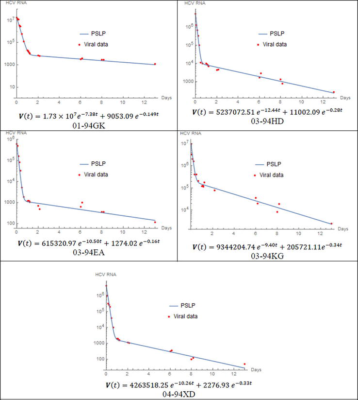
To demonstrate the capabilities and proficiency of the proposed method, four case studies are presented. These cases involve the examination of viral kinetics using the standard mathematical model of HCV dynamics. The PSLP method is utilized to solve the nonlinear dynamic model of viral kinetics for certain patients following the initiation of treatment with DAAs. In order to evaluate the performance of the PSLP method, the predictions are compared, for each patient, with viral load data found in literature sources [29, 30]. To obtain the best fit of data for each patient, parameters $\delta ,\epsilon ,c$, and $\rho$ are estimated by utilizing Eq. (10) and the initial condition relation given in Eq. (4). The first case study examines patients who have been infected with HCV genotype 1 and treated with danoprevir. The viral load for these patients is monitored for 13 days after the initiation of danoprevir, and the data are available in [29]. The parameters are given in Table 1, and Figure 1 demonstrates the comparison between the solution of PSLP method and the corresponding viral load data for each patient.

Patient	$V_0$ (IU/mL)	$c$ (day)^−1	$\epsilon$	$\delta$ (day)^−1	$\rho$ (day)^−1
01-94GK	${10}^{7.24}$	$7.38$	$0.9995$	$0.15$	149.684
03-94HD	${10}^{6.72}$	$12.44$	$0.998$	$0.29$	151.188
03-94EA	${10}^{5.79}$	$10.5$	$0.998$	$0.17$	11.212
03-94KG	${10}^{6.98}$	$9.4$	$0.98$	$0.35$	246.748
04-94XD	${10}^{6.63}$	$10.26$	$0.9995$	$0.33$	116.31

Table 1.

Parameter values used for the patients treated with danoprevir.

Figure 1.

Comparison between the approximate analytical solution using PSLP method and viral data for patients treated with danoprevir. $s=1.3\ast {10}^5$cells/ml, $d=0.01{\mathrm{day}}^{-1}$, $\beta =5\ast {10}^{-8}$ ml ${\mathrm{day}}^{-1}{\text{virion}}^{-1}$, and the rest of parameter values are given in Table 1.

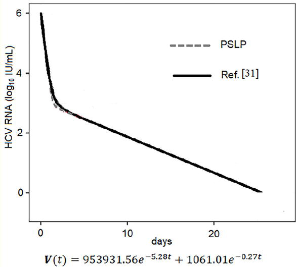
Another case study is presented, which examines an exploited combination of multi-drug DAAs treatments. The predictions of the PSLP method are compared with the corresponding viral load data obtained through simulation in [31]. The parameter values used in this case are listed in Table 2, with $\delta ,\epsilon ,\text{and}c$ having the same values assigned in [31], and $\rho$ chosen accordingly. Figure 2 displays the PSLP results and the published simulation results for 25 days after the initiation of treatment with TVR + PR. The PSLP solution and the simulation results are highly similar. This comparison demonstrates that the proposed PSLP method can provide appropriate approximate analytical solutions for all considered cases. It is worth mentioning that in this case, the rate of cure is close to 100%.

DAAs	$c_{V_0}$ (IU/mL)	$c$ (day)^−1	$\epsilon$	$\delta$ (day)^−1	$\rho$ (day)^−1
TVR + PR	${10}^{5.98}$	$5.28$	$0.999$	$0.27$	8.18

Table 2.

Parameter values used with TVR + PR.

Figure 2.

Comparison between results obtained by PSLP method and by simulation in [31] for treatment with TVR + PR. $s=1.3\times {10}^5$cells/ml, $d=0.01{\mathrm{day}}^{-1}$, $\beta =5\times {10}^{-8}$ ml ${\mathrm{day}}^{-1}{\text{virion}}^{-1}$. Table 2 Gives the values for the rest of parameter.

The PSLP solution provides a valuable tool for medical specialists and physicians to predict a patient’s response to a specific treatment regimen before the treatment begins. They can use the patient’s parameters to calculate the constants in Eq. (9) and Eq. (11) and substitute them in Eq. (10) to obtain a closed-form solution for the viral load. This allows them to plot the viral load over time or estimate the viral load at any given point in time by direct substitution in the closed-form solution. The ability to predict a patient’s response to treatment before it starts is highly desirable for efficient and effective medical care.

3. Classical PDEs multiscale model

A multiscale model in the form of PDEs, which describes the intracellular life cycle had been proposed and applied by many researchers to analyze clinical data under multidrug treatment [29, 30, 31, 32, 33]. The model is as follows:

$$\frac{\partial R\left(a,t\right)}{\partial t}+\frac{\partial R\left(a,t\right)}{\partial a}=\alpha \left(1-{\epsilon }_{\alpha }\right)-\left(\left(1-{\epsilon }_s\right)\rho +\mathit{k\mu }\right)R\left(a,t\right)$$E12

$$\frac{\mathit{dT}\left(t\right)}{\mathit{dt}}=s-dT\left(t\right)-\beta V\left(t\right)T\left(t\right)$$E13

$$\frac{\partial i\left(a,t\right)}{\partial t}+\frac{\partial i\left(a,t\right)}{\partial a}=-\delta i\left(a,t\right)$$E14

$$\frac{\mathit{dV}\left(t\right)}{\mathit{dt}}=\left(1-{\epsilon }_s\right)\rho \underset{0}{\overset{\infty }{\int }}R\left(a,t\right)i\left(a,t\right)\mathit{da}-cV\left(t\right)$$E15

with the following boundary conditions: $R\left(0,t\right)=\mathrm{\zeta }$, $i\left(0,t\right)=\beta V\left(t\right)T\left(t\right).$ $R\left(a,t\right)$ is the age and time distribution of intracellular viral RNA (vRNA) in a cell with infection age $a$. The parameters $\alpha$ and $\mathrm{\mu }$ represent the production and degradation rates of intracellular vRNA, respectively. It is assumed that vRNA assembles with viral proteins and is released from an infected cell as viral particles at a rate of ρ. The efficacies ${\epsilon }_{\alpha },$ ${\epsilon }_s$, and $k$ play a role in inhibiting intracellular viral production, preventing the assembly and/or secretion of virions, and increasing the degradation rate of vRNA, respectively. The entry virus-derived RNA starts to replicate from ζ copies in a newly infected cell.

4. Transformed ODEs multiscale model

Kitagawa et al. [34, 35] transformed the previous multiscale PDEs model into a mathematically alike ODEs model without any assumptions. The transformed model can be written as:

$$\frac{\mathit{dT}\left(t\right)}{\mathit{dt}}=s-dT\left(t\right)-\beta V\left(t\right)T\left(t\right)$$E16

$$\frac{\mathit{dI}\left(t\right)}{\mathit{dt}}=\beta V\left(t\right)T\left(t\right)-\delta I\left(t\right)$$E17

$$\frac{\mathit{dP}\left(t\right)}{\mathit{dt}}=\mathrm{\zeta }\beta V\left(t\right)T\left(t\right)+\alpha \left(1-{\epsilon }_{\alpha }\right)I\left(t\right)-\left(\mathit{k\mu }+\rho \left(1-{\epsilon }_s\right)+\delta \right)P\left(t\right)$$E18

$$\frac{\mathit{dV}\left(t\right)}{\mathit{dt}}=\rho \left(1-{\epsilon }_s\right)P\left(t\right)-cV\left(t\right)$$E19

where $I\left(t\right)$ denotes the total number of infected cells and defined as $I\left(t\right)=\underset{0}{\overset{\infty }{\int }}i\left(a,t\right)\mathit{da}$, and $P\left(t\right)$ is the total amount of intracellular vRNA pooled in all infected cells and defined as $P\left(t\right)=\underset{0}{\overset{\infty }{\int }}R\left(a,t\right)i\left(a,t\right)\mathit{da}$.

5. ODEs multiscale model incorporating cell proliferation

The transformed model can predict a biphasic decline for the viral load. It cannot predict a triphasic viral decay. To explain this, let us first assume the existence of a shoulder viral load and then prove that this is not possible for the model. For the shoulder, we can consider $V\left(t\right)$ as constant, that means that $\frac{\mathit{dV}\left(t\right)}{\mathit{dt}}=0$, which can be substituted to Eq. (19) to get that $P\left(t\right)$ is also constant which means that $\frac{\mathit{dP}\left(t\right)}{\mathit{dt}}=0$. Since $T\left(t\right)$ is increasing, Eq. (18) indicates that $I\left(t\right)$ is decreasing. If these are substituted in Eq. (17), it means that $\frac{\mathit{dI}\left(t\right)}{\mathit{dt}}$ is increasing. However, since $I\left(t\right)$ is always positive, pointing that $\frac{\mathit{dI}\left(t\right)}{\mathit{dt}}$ is increasing is in contradiction with $I\left(t\right)$ decreasing. Hence, the transformed model presented in (2) cannot predict the shoulder phase. It is worth mentioning that whatever is confirmed for the transformed model is also confirmed for the classical multiscale model presented by Eq. (12)–Eq. (15).

The transformed ODE model ignores proliferation of both infected and uninfected cells, though hepatocytes have been suggested to be the major producers of HCV. We assume that target cells are hepatocytes and suggested to include the density-dependent proliferation terms for both infected and uninfected hepatocytes that only allow growth of the liver until a maximum size, $T_{\mathit{max}}$, is reached.

5.1 Mathematical model

The extended model is given by:

$$\frac{\mathit{dT}\left(t\right)}{\mathit{dt}}=s-dT\left(t\right)-\beta V\left(t\right)T\left(t\right)+\mathit{rT}\left(t\right)\left(1-\frac{T\left(t\right)+I\left(t\right)}{T_{\mathit{max}}}\right)$$E20

$$\frac{\mathit{dI}\left(t\right)}{\mathit{dt}}=\beta V\left(t\right)T\left(t\right)-\delta I\left(t\right)+\mathit{rI}\left(t\right)\left(1-\frac{T\left(t\right)+I\left(t\right)}{T_{\mathit{max}}}\right)$$E21

$$\frac{\mathit{dP}\left(t\right)}{\mathit{dt}}=\mathrm{\zeta }\beta V\left(t\right)T\left(t\right)+\alpha \left(1-{\epsilon }_{\alpha }\right)I\left(t\right)+\mathrm{\zeta }rI\left(t\right)\left(1-\frac{T\left(t\right)+I\left(t\right)}{T_{\mathit{max}}}\right)-\left(\mathit{k\mu }+\left(1-{\epsilon }_s\right)\rho +\delta \right)P\left(t\right)$$E22

$$\frac{\mathit{dV}\left(t\right)}{\mathit{dt}}=\left(1-{\epsilon }_s\right)\mathit{\rho P}\left(t\right)-cV\left(t\right)$$E23

where uninfected $T\left(t\right)$ and infected $I\left(t\right)$ hepatocytes can proliferate with maximum proliferation rate $r$, under a blind homeostasis process, in which there is no distinction between infected and uninfected cells in the density-dependent term. The logistic terms describe the proliferation of the uninfected cells $T$ and the proliferation of the infected cells $I$ that are limited by the maximum size $T_{\mathit{max}}$. Hence, the saturation effects of both the uninfected and the infected cells are contained in the model. Therefore, the model could not predict unrealistic unlimited increases in the values of these cells. Also, it can be noticed that the proliferation terms assumes that the growth rate decreases linearly with the increase of the total hepatocytes population $T\left(t\right)+I\left(t\right)$ until it reaches zero at the maximum size.

By inclusion of proliferation of hepatocytes in the extended model, the model can predict viral kinetics in chronic HCV patients during and after antiviral therapy. The shoulder phase, and hence a triphasic viral decay, occurs if the number of uninfected cells is much lower than the number of infected cells before therapy, and the rate of proliferation plus the rate of de novo of infected cells equals the rate of infected cell loss. As the number of uninfected cells increase, proliferation of infected cells slows and ultimately reaches a point at which the number of infected cells starts to decline. Hence, the third phase of viral decline starts.

Unlike the transformed model which predicts virus resurgence to pretreatment levels with damped oscillations after cessation of therapy, the extended model predicts virus resurgence to pretreatment levels without oscillations after cessation of therapy, as can be seen in the following sections. The kinetics of viral resurgence thus tends to mimic that observed in patients taken off therapy.

The model incorporating cell proliferation can predict both a biphasic decline and a triphasic decline. To prove this, we assume the existence of a shoulder viral load and then confirm that this is possible for the extended model. For the extended model, let $V\left(t\right)$ be constant at the shoulder which means that $\frac{\mathit{dV}\left(t\right)}{\mathit{dt}}=0$ and substitute into the fourth equation in model (3) to get that $P\left(t\right)$ is also constant which means that $\frac{\mathit{dP}\left(t\right)}{\mathit{dt}}=0$. For the third equation in this model, it is not a must that $I\left(t\right)$ is decreasing since $T\left(t\right)$ is increasing because the proliferation term is decreasing and can compensate for the increase in $T\left(t\right)$ even if $I\left(t\right)$ is constant. The same argument is applied for the second equation in model (3), and the increase in the first term can be compensated by the decrease in the proliferation term. Hence, for constant $I\left(t\right)$, the model (3) can predict $\frac{\mathit{dI}\left(t\right)}{\mathit{dt}}=0$. Therefore, the model can predict the shoulder phase for the viral load.

5.2 Biphasic and triphasic viral decline

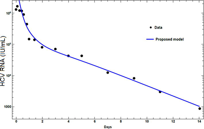
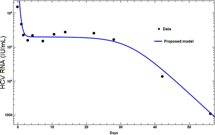
The results from the proposed model are compared with the published experimental data. Experimental HCV RNA data, for two patients treated with peginterferon α-2a alone [17, 24], and in combination with ribavirin [23, 25], are presented. The values assigned for the parameters for each patient are given in Table 3. The first patient exhibits a biphasic decline. Figure 3, for a patient treated with peginterferon α-2a alone, shows that the viral load has a phase of rapid decline at the beginning followed by a phase of normal decline. The second patient, treated with peginterferon α-2a in combination with ribavirin, exhibits triphasic decline. The triphasic decline consists of a first phase with rapid virus load decline, followed by a shoulder phase in which virus load decays slowly, and a third phase of renewed normal viral decay as can be seen in Figure 4. Figures 3 and 4 show that the proposed model can present both the biphasic and the triphasic viral decline, and it can be noticed that the proposed model is consistent with the data.

Parameter	Patient 1	Patient 2	Units
$T_{\mathit{max}}$	$0.7\times {10}^7$	$0.6\times {10}^7$	$\text{cell}{\mathrm{ml}}^{-1}$
$s$	$8\times {10}^5$	$0.62\times {10}^3$	$\text{cell}{\mathrm{ml}}^{-1}{\mathrm{day}}^{-1}$
$\beta$	$0.6\times {10}^{-7}$	$0.5\times {10}^{-7}$	$\mathrm{ml}{\mathrm{day}}^{-1}{\text{virion}}^{-1}$
$d$	$4.7\times {10}^{-3}$	$8.7\times {10}^{-3}$	${\mathrm{day}}^{-1}$
$\delta$	$0.3$	$0.24$	${\mathrm{day}}^{-1}$
$c$	$5.9$	$4.4$	${\mathrm{day}}^{-1}$
$r$	$0.45$	$0.5$	${\mathrm{day}}^{-1}$
$\rho$	5.4	6.3	${\mathrm{day}}^{-1}$
$\mathrm{\zeta }$	1	1	$\mathit{\text{viron}}{\mathit{\text{cell}}}^{-1}$
$\alpha$	$14$	$21$	$\mathit{\text{viron}}{\mathit{\text{cell}}}^{-1}{\mathrm{day}}^{-1}$
$\mu$	$1$	$1$	${\mathrm{day}}^{-1}$
${\epsilon }_s$	$0.906$	$0.899$
$k$	$1$	$1$
${\epsilon }_{\alpha }$	$0.97$	$0.972$

Table 3.

Parameter values used in fitting model with HCV RNA data of patients.

Figure 3.

Fitting viral loads from the model with experimental data for patient 1.

Figure 4.

Fitting viral loads from the model with experimental data for patient 2.

5.3 Viral kinetics after treatment cessation

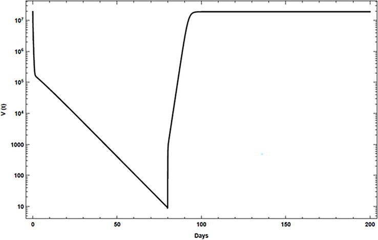
In most treated individuals, the virus returns to its pretreatment levels within 1–2 weeks after cessation of treatment [23]. To consider this phenomenon, the drug efficacies ${\epsilon }_{\alpha }\mathit{\text{and}}{\epsilon }_s$ are assigned at time 0 for 80 days, as given in Table 4, and then these efficacies are set to 0 for the rest of the simulation. Figure 5 shows that with the inclusion of proliferation in the proposed model, the virus returns to its pretreatment level quickly.

Parameter	Value and units	Parameter	Value and units
$s$	$13\times {10}^5\text{cell}{\mathrm{ml}}^{-1}{\mathrm{day}}^{-1}$	$\alpha$	$40\mathit{\text{viron}}{\mathit{\text{cell}}}^{-1}{\mathrm{day}}^{-1}$
$\beta$	$5\times {10}^{-8}\mathrm{ml}{\mathrm{day}}^{-1}{\text{virion}}^{-1}$	$\mu$	$1{\mathrm{day}}^{-1}$
$d$	$0.1{\mathrm{day}}^{-1}$	$c$	$22.3{\mathrm{day}}^{-1}$
$T_{\mathit{max}}$	$1.35\times {10}^7\text{cell}{\mathrm{ml}}^{-1}$	$\rho$	8.18 ${\mathrm{day}}^{-1}$
$r$	$2.4{\mathrm{day}}^{-1}$	$k$	$1$
$\delta$	$0.14{\mathrm{day}}^{-1}$	${\epsilon }_{\alpha }$	$0.99$
$\mathrm{\zeta }$	1 $\mathit{\text{viron}}{\mathit{\text{cell}}}^{-1}$	${\epsilon }_s$	$0.56$

Table 4.

Parameter values used in the numerical simulation.

Figure 5.

Simulation of viral kinetics after therapy cessation using the model, case 1.

5.4 Discussion

The model explores the dynamics of HCV infection under therapy with DAAs including both the intracellular viral RNA replication/degradation and the extracellular viral infection with age dependency and time dependency. The model consists of a system of nonlinear ODEs instead of PDEs in classical multiscale model. Therefore, numerical computation is more efficient, time-saving, and convergent.

Numerical studies prove that the model can represent the triphasic patterns profile in HCV RNA decay which had been recorded for a class of patients. It can also represent the viral rebound to pretreatment levels after therapy cessation without oscillation. Moreover, agreement of the model with experimental data is confirmed.

6. ODE multiscale model incorporating body immune system

An extension to the transformed multiscale ODE model is presented. Two additional variables are included in the transformed model to account for the immune system response. The first variable, $Z\left(t\right)$, represents the number of CTLs, which are responsible for destroying infected cells and thereby inhibiting the reproduction of the virus. The second variable, $W\left(t\right)$, represents the number of antibodies generated, which play a role in neutralizing the virus in vivo.

6.1 Mathematical model

The new model is described by the following ODEs system:

$$\frac{\mathit{dT}\left(t\right)}{\mathit{dt}}=s-rT\left(t\right)-\beta V\left(t\right)T\left(t\right)$$E24

$$\frac{\mathit{dI}\left(t\right)}{\mathit{dt}}=\beta V\left(t\right)T\left(t\right)-\delta I\left(t\right)-fI\left(t\right)Z\left(t\right)$$E25

$$\frac{\mathit{dP}\left(t\right)}{\mathit{dt}}=\beta V\left(t\right)T\left(t\right)+\alpha \left(1-{\epsilon }_{\alpha }\right)I\left(t\right)-\left(\mathit{k\mu }+\left(1-{\epsilon }_s\right)\rho +\delta \right)P\left(t\right)$$E26

$$\frac{\mathit{dV}\left(t\right)}{\mathit{dt}}=\rho \left(1-{\epsilon }_s\right)P\left(t\right)-cV\left(t\right)-qV\left(t\right)W\left(t\right)$$E27

$$\frac{\mathit{dZ}\left(t\right)}{\mathit{dt}}=uI\left(t\right)Z\left(t\right)-bZ\left(t\right)$$E28

$$\frac{\mathit{dW}\left(t\right)}{\mathit{dt}}=\mathit{gV}\left(t\right)W\left(t\right)-hW\left(t\right)$$E29

The term $fI\left(t\right)Z\left(t\right)$ in Eq. (25) represents the rate at which infected cells are killed by the CTL response, and the term $qV\left(t\right)W\left(t\right)$in Eq. (27) represents the rate at which virus particles are neutralized by the antibodies. CTLs become activated in response to viral antigens from infected cells and once activated, they divide and their population grows (clonal expansion). Therefore, in Eq. (28), CTLs increase at a rate of $\mathit{uI}\left(t\right)Z\left(t\right)$ and decay at a rate of $\mathit{bZ}\left(t\right)$ due to the lack of antigenic stimulation. Antibodies are produced by B cells and are initially attached to them, serving as receptors that can recognize the virus. When B cells are exposed to a free virus, they divide and secrete the antibodies. Thus, antibodies progress at a rate $\mathit{gV}\left(t\right)W\left(t\right)$ and decay at a rate $\mathit{hW}\left(t\right)$ in Eq. (29).

6.2 Basic reproduction number

The basic reproduction number, denoted as $R_0$, is defined as the expected total number of viral particles newly produced during the entire period of infection from one typical viral particle in a population consisting only of uninfected cells. It is calculated under no treatment conditions and is also computed at the disease-free equilibrium point $E_0$. No treatment can be specified by assigning ${\epsilon }_{\alpha }=0$, ${\epsilon }_s=0,\text{and}k=1$ in the presented model, and $E_0$will be obtained in the following section. This basic reproduction number explains the average number of newly infected cells based on the dynamics of the total amount of intracellular viral RNA, which corresponds to $P\left(t\right)$ in the transformed ODE model, instead of the dynamics of the individual amount of intracellular viral RNA in the original PDE model. Note that the life cycles of both extracellular viral and total intracellular viral RNA are explicitly considered in the ODE model, and the viruses are formulated from the viral RNAs.

There are several methods that can be used to obtain the basic reproduction number, such as the next-generation method, which was introduced by Diekmann et al., [37]. There are two main approaches to apply this method, as explained by Driessche and Watmough [38] and by Castillo-Chavez, et al., [39]. In this work, the second approach is used, and proofs and further details can be found in [38, 39, 40]. The obtained form for $R_0$ is given by:

$$R_0=\frac{\beta s\rho \left(\alpha +\delta \right)}{cr\delta \left(\mu +\rho +\delta \right)}$$E30

6.3 Equilibrium points

Equilibrium points are the values of the variables $T_{\ast },I_{\ast },P_{\ast },V_{\ast },Z_{\ast }$, and $W_{\ast }$, under no treatment, at which the derivatives of these variables, i.e., the left-hand sides in Eq. (24)–Eq. (29), vanish. These equilibrium points represent the steady state values of the variables after the cease of medication. In fact, in stability analysis, the interest is in specifying the behavior of the virus after the cease of medication. Commercial program Mathematica 12 program is used to solve these algebraic equations. The program gives six equilibrium points; however, one of them has negative coordinates that have no biological meaning. The five other points are as follows:

$$E_0=\left(\frac{s}{r},0,0,0,0,0\right)$$E31

$$E_1=\left(\frac{s}{r{R}_0},\frac{s}{\delta }\left(1-\frac{1}{R_0}\right),\frac{cr}{\mathit{\beta \rho }}\left(R_0-1\right),\frac{r}{\beta }\left(R_0-1\right),0,0\right)$$E32

$$E_2=\left(k_{2}s,\frac{\mathit{\beta h}\mathrm{S}}{\mathit{\delta g}}{k}_2,\frac{crh{R}_0}{\mathit{g\rho }}{k}_2,\frac{h}{g},0,\frac{c}{q}\left(-1+r{k}_2{R}_0\right)\right)$$E33

$$E_3=\left(\frac{k_1+2cru{\mathrm{\mu }}_1-k_3}{2\beta r\mathit{\rho u}},\frac{b}{u},\frac{k_1+k_3}{2\beta \rho {\mathrm{\mu }}_{1}u},\frac{k_1+k_3}{2\beta c{\mathrm{\mu }}_{1}u},\frac{\left(k_1+k_3\right)}{2b\mathit{\beta \rho f}}-\frac{\left(\alpha +\delta \right)}{f},0\right)$$E34

$$E_4=\left(k_{2}s,\frac{b}{u},\frac{\mathit{c\delta }r{R}_0}{\mathit{s\rho }\left(\alpha +\delta \right)}\left(\frac{\alpha b}{u\beta }+\frac{s{k}_{2}h}{g}\right),\frac{h}{g},\left(\frac{\beta hsu}{\mathit{\text{brgf}}+\mathit{\text{bβhf}}}-\frac{\delta }{f}\right),\left(\frac{\alpha \mathit{bg\rho }}{h{\mathrm{\mu }}_1\mathit{qu}}+\frac{\beta k_2\mathit{\rho s}}{{\mathrm{\mu }}_{1}q}-\frac{c}{q}\right)\right)$$E35

where

$${\mathrm{\mu }}_1=\left(\delta +\mu +\rho \right)k_1=\alpha b\beta \rho +\mathit{\beta \rho }\mathrm{s}u-cru{\mathrm{\mu }}_1{k}_2=\frac{g}{rg+\mathit{\beta h}}$$E36

$$k_3=\sqrt{4\alpha b\beta cr\rho {\mathrm{\mu }}_{1}u+{k_1}^2}$$

The first point, $E_0$, is a virus-free equilibrium point, while the other four points are virus-infected. These four infected equilibrium points are an infected state with no immune responses, an infected state with dominant antibody responses without CTLs, an infected state with dominant CTL responses without antibodies, and an infected state with coexistence responses of both CTLs and antibodies, respectively.

6.4 Stability analysis

Global stability analysis of a dynamical system is a very complex problem. One of the most efficient methods to solve this problem is Lyapunov’s theory. To build the Lyapunov function, the technique used in [22, 41], which had been suggested and utilized for other dynamical models, is adopted. The global asymptotic stability of the model for both the uninfected and the infected equilibrium points is investigated and the following stability theorem has been proven:

1. $E_0$ is globally asymptotically stable if $R_0\le 1.$

2. $E_1$ is globally asymptotically stable if $1\le R_0\le \mathit{min}\left(A_1,A_2\right)$.

3. $E_2$ is globally asymptotically stable if $A_1\le R_0\le A_3$.

4. $E_3$ is globally asymptotically stable if $A_2\le R_0\le A_4$.

5. $E_4$ is globally asymptotically stable if $R_0\ge \mathit{max}\left(A_3,A_4\right)$.

where.

$$A_1=1+\frac{\beta h}{rg},A_2=1+\frac{\beta \rho b\left(\alpha +\delta \right)}{cru{\mu }_1},A_3=\frac{\mathit{g\rho }b\left(\alpha +\delta \right)}{cruh{k}_2{\mu }_1},\text{and}{A}_4=\frac{\beta suh\left(\alpha +\delta \right)}{r\delta \left(\alpha bg+\beta suh{k}_2\right).}$$E37

Details can be found in [42].

6.5 Simulations

The model is numerically simulated. Mathematica 12 program is utilized to solve the system of ODEs numerically. The simulations are performed using parameters estimated from clinical datasets in [34]: $\beta =5\times {10}^{-8}\mathrm{ml}{\mathrm{day}}^{-1}{\text{virion}}^{-1},r=0.01{\mathrm{day}}^{-1},\delta =0.14{\mathrm{day}}^{-1},\alpha =40{\mathrm{day}}^{-1},k=1{\mathrm{day}}^{-1},\mathrm{\mu }=1{\mathrm{day}}^{-1},\rho =8.18{\mathrm{day}}^{-1},{\epsilon }_{\alpha }=0.99,{\epsilon }_s=0.56.$ The immune system parameters are proposed in [26] as: $u=4.4\times {10}^{-7}{\mathrm{day}}^{-1},b={10}^{-2}{\mathrm{day}}^{-1},g={10}^{-5}{\mathrm{day}}^{-1},h={10}^{-2}{\mathrm{day}}^{-1},f=6.4\times {10}^{-4}{\mathrm{day}}^{-1},q=2{\mathrm{day}}^{-1}.$ The units for $s$ is cells/ml.${\mathrm{day}}^{-1}$, and the units for $c\text{is}{\mathrm{day}}^{-1}.$ Some parameters are not given in Table 5, and the used values will be given explicitly.

	$s$	c	$R_0$	$A_1$	$A_2$	$A_3$	$A_4$
case 1	$1.3\times {10}^4$	$22.3$	$0.733$
case 2	68,225	$82.3$	$1.043$	$1.05$	$1.049$	$1.02$	$1.07$
case 3	$1.3\times {10}^5$	$22.3$	$7.33$	$1.005$	$1.18$	$36.08$	$0.204$
case 4	$1.3\times {10}^5$	$82.3$	$1.99$	$1.05$	$1.049$	$1.021$	$2.036$
case 5	$1.3\times {10}^6$	$22.3$	$73.35$	$1.005$	$1.18$	$36.08$	$2.036$

Table 5.

Cases considered in the simulation.

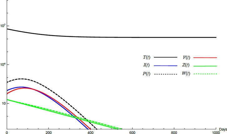
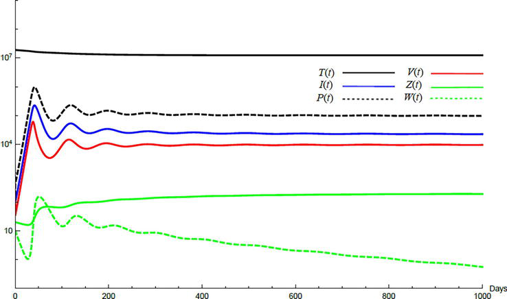
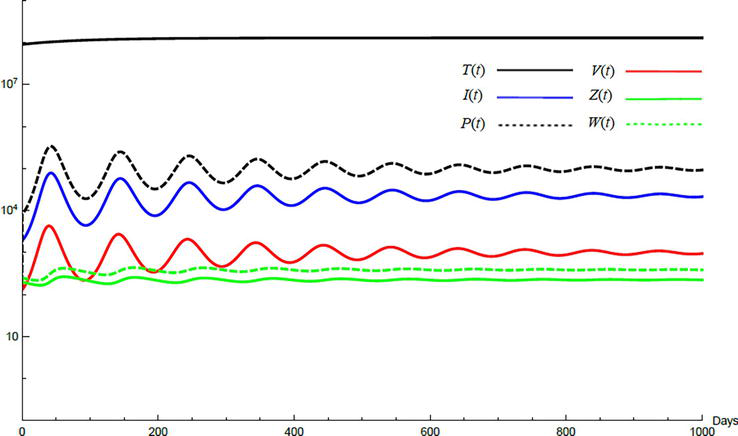
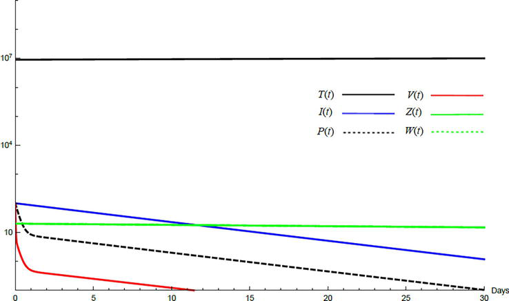
Simulations demonstrate the mutual relations between the basic reproduction number, the equilibrium points, and the stability analysis. The variations of all variables $T\left(t\right),I\left(t\right),P\left(t\right),V\left(t\right),Z\left(t\right),W\left(t\right)$ with time are obtained. Each figure represents a case with a specific value for the basic reproduction number $R_0$ which leads to a corresponding equilibrium point that is stable according to the stability theorem given in the previous subsection. The model under no treatment is simulated first, and it is obtained by assigning ${\epsilon }_{\alpha }=0$, ${\epsilon }_s=0,\text{and}k=1$ in Eq. (24)–Eq. (29). The cases are given in Table 5. Figures 6–10 illustrate that the variables converge to the values of the corresponding equilibrium point. $T^0,I^0,P^0,V^0,Z^0,\text{and}{W}^0$ are the initial values of the variables.

Figure 6.

Variation of the variables for no treatment case 1. Hence, $R_0<1$ and $E_0$ is stable; $E_0=\left\{1.3\times {10}^6,0,0,0,0,0\right\}$. $T^0=0.6\times {10}^7,I^0=100,P^0=400,V^0=50,Z^0=20,W^0=20.$

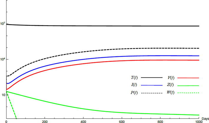
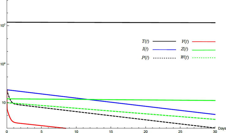
Figure 7.

Variation of the variables for no treatment case 2. Hence, $1<R_0<\mathit{min}\left(A_1,A_2\right)$ and $E_1$ is stable; $E_1=\left\{6.54\times {10}^6,20108,86603,8608,0,0\right\}.T^0=0.9\times {10}^7,I^0=100,P^0=100,V^0=100,Z^0=20,W^0=20.$

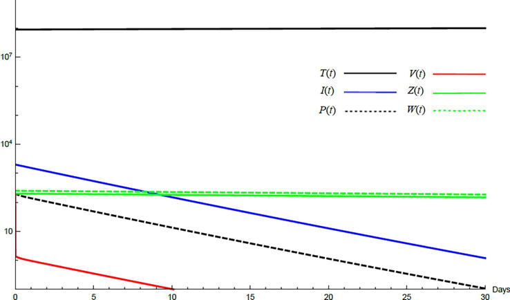
Figure 8.

Variation of the variables for no treatment case 3. Hence, $A_1<R_0<A_3$ and $E_2$ is stable; $E_2=\left\{1.29\times {10}^7,4620,19897,1000,0,70\right\}$. $T^0=0.9\times {10}^7,I^0=100,P^0=100,V^0=100,Z^0=20,W^0=20.$

Figure 9.

Variation of the variables for no treatment case 4. Hence, $A_2<R_0<A_4$ and $E_3$ is stable; $E_3=\left\{1.24\times {10}^7,22727,98191,9759,197,0\right\}.T^0=1.9\times {10}^7,I^0=100,P^0=100,V^0=100,Z^0=20,W^0=20.$

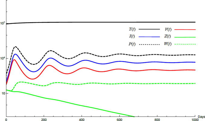
Figure 10.

Variation of the variables for no treatment case 5. Hence, $R_0\ge \mathit{max}\left(A_3,A_4\right)$ and $E_4$ is stable; $E_4=\left\{1.29\times {10}^8,22727,98236,1000,226,391\right\}$. $T^0=0.9\times {10}^8,I^0=2000,P^0=200,V^0=200,Z^0=200,W^0=250$.

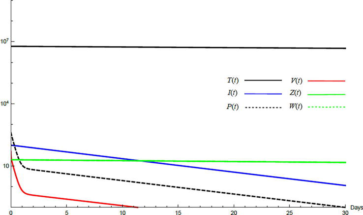
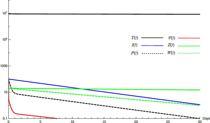
To demonstrate the effect of medical treatments, the model with treatment presented by Eq. (24)–Eq. (29) is considered. The same five cases are reconsidered, however, with medical treatment. The effect of medication is reveled in Figures 11–15. Whenever the curve for the antibodies is not seen, it coincides with the curve for CTLs. The simulation proves the practicality and the effectiveness of the proposed model.

Figure 11.

Variation of the variables for medical treatment case 1.

Figure 12.

Variation of the variables for medical treatment case 2.

Figure 13.

Variation of the variables for medical treatment case 3.

Figure 14.

Variation of the variables for medical treatment case 4.

Figure 15.

Variation of the variables for medical treatment case 5.

6.6 Discussion

The parameters related to the immune system do not impact the basic reproduction number, as shown in Eq. (30). When a virus particle is introduced to a population of uninfected cells $T$, the virus infects some of the cells $I$ and produces intracellular viral RNA $P$. However, without the presence of CTLs and antibodies, they cannot be generated. Therefore, the parameters represented by $Z$and $W$ are not present in the formula for $R_0$.

There are now five equilibrium points. The first is a virus-free state, and the second is an infected state with no immune response. These two points are the same as those obtained using a model without the immune system [35]. The three infected equilibrium points include a state with dominant antibody response and no CTL response, a state with dominant CTL response and no antibody response, and a state with coexistence of both CTLs and antibodies. The CTLs and antibodies are in competition, with the role of CTLs and antibodies in resolving HCV infection being debated in the literature [43, 44]. The infected equilibrium point with dominant antibody response means that the antibody response is strong and reduces the virus load to a level where the CTL response is not stimulated. Similarly, the infected equilibrium point with dominant CTL response means that the CTL response is strong and reduces the virus load to a level where the antibody response is not stimulated. In these two equilibrium points, one of the responses is excluded due to competition between them. The competition may also result in the coexistence of both responses, as seen in the fifth equilibrium point.

Comparing the values of the variables $T_{\ast },I_{\ast },P_{\ast },\text{and}{V}_{\ast }$ for the equilibrium point with no immune response $E_1$ and the equilibrium point with dominant antibody response $E_2$, it can be seen that that $T_2\ge T_1$, $I_2\le I_1$, $P_2\le P_1$, and $V_2\le V_1$ when $E_2$ exists, i.e., $R_0\ge A_1$. The same is true for the equilibrium point with dominant CTL response $E_3$ and the equilibrium point with coexistence of both CTLs and antibodies $E_4$. While the antibody and CTL responses may not completely eliminate the viral load, they significantly increase the number of uninfected cells, decrease the number of infected cells and intracellular viral RNA, and reduce the viral load.

It is important to note that the stability theorem in subsection 6.4 indicates that each equilibrium point has a specific domain of stability. These domains can overlap. For example, if $A_1\le A_2$ and $A_3\le A_4$, the domains of global stability of $E_2$ and $E_3$ will be intersecting except if $A_3\le A_2$. This can result in a bistable equilibrium, where two stable equilibrium points coexist. This has been reported in many biological situations, such as in multistrain disease dynamics [40], in low capacity for the treatment of infective in epidemic models [45], and in the investigation of bifurcations and stability of an HIV model that incorporates immune responses [46]. In the presence of bistable equilibrium, the solution converges to one of the two stable equilibrium points depending on the initial conditions, which is called bistable dominance.

The proposed model is a multiscale model that incorporates the immune system response and considers intracellular viral RNA replication and degradation with age dependency in addition to time dependency. This allows the model to explore the dynamics of HCV infection under therapy with DAAs by including both intracellular viral RNA replication/degradation and extracellular viral infection with age dependency in addition to time dependency. The parameter $P$, which represents the intracellular viral RNA, appears in both the basic reproduction number and the coordinates of the equilibrium points.

7. Conclusion

Power series solution combined with Laplace-Padé resummation method (PSLP) have been used to obtain a general approximate analytical solution for the standard model of HCV for patients treated with DAAs. Results have been compared with experimental viral load data and with published simulated results. The comparison proves that this innovative PSLP solution can be used with confidence for solving the nonlinear standard viral dynamic model. This solution can conveniently be used to fit patient data and estimate parameter values.

An ODEs multiscale model incorporating cell proliferation has been presented. The model has the advantages of both multiscale model and models account for proliferation. Hence, the model includes the major stages in the HCV life cycle that are targeted by DAAs and can also explain some observed behavior in viral kinetic. It can improve our understanding of this biological process including therapy effects. The model eliminates two main limitations in the classical multiscale model and its transformed model, namely, the impossibility to fit the viral load of those patients who show a triphasic profile in virus decay, and lake of representing viral rebound to baseline values after the cessation of therapy. Remarkably, the results of the model have been compared with experimental data reported in the literature, and these results have been fitted to these data.

A multiscale model incorporating the immune system, which plays a crucial role in lowering the virus load, has been developed for understanding and managing chronic HCV. This model offers several benefits over traditional models, including the ability to determine equilibrium points after medication cessation in the presence of immune effects. The parameters related to the immune system do not impact the basic reproduction number, and the disease-free and endemic equilibrium points have been identified. The conditions for their existence have also been determined. The model has a maximum of five total equilibrium points, including the uninfected point, with the four infected equilibrium points being dependent on immune system parameters.

It has been shown that the uninfected equilibrium point is stable if $R_0$ ≤ 1 and unstable if $R_0$ > 1. The stability of the infected equilibrium points is based on both the basic reproduction number and the parameters associated with the CTL response and antibody response, which play a critical role in determining equilibrium point stability. Activation of antibodies and CTLs can effectively reduce the viral load but not completely eliminate it.

For effective treatment, if $R_0>1$, the focus should be on improving the body’s parameters to bring $R_0\le 1$. Once this is achieved, treatment to reduce the virus can be implemented until the body reaches the stable uninfected equilibrium point. This will allow the immune system to lead the body to a stable uninfected state. On the other hand, if an unstable uninfected equilibrium point exists, the virus cannot be eliminated even if the uninfected point is approached. Additionally, successful treatment also means that infected equilibrium points do not exist, so the system will not be drawn to any of them if they were to exist.

References

1.Jefferies M, Rauff B, Rashid H, Lam T, Rafiq S. Update on global epidemiology of viral hepatitis and preventive strategies. World Journal of Clinical Cases. 2018;6(13):589-599
2.Hepatitis: Key Facts. World Health Organization 2022. Available from: https://www.who.int/news-room/fact-sheets/detail/hepatitis-c[Accessed November 13, 2022]
3.Carithers RL, Emerson SS. Therapy of hepatitis C: Meta-analysis of interferon alfa-2b trials. Hepatology. 1997:26S3
4.McHutchison JG, Gordon SC, Schiff ER, Shiffman ML, Lee WM, Rustgi VK, et al. Interferon alfa-2b alone or in combination with RIBAVIRIN as initial treatment for chronic Hepatitis C. New England Journal of Medicine. 1998;339:1485-1492
5.Poynard T, McHutchison J, Manns M, Trepo C, Lindsay K, Goodman Z, et al. Impact of pegylated interferon alfa-2b and ribavirin on liver fibrosis in patients with chronic hepatitis C. Gastroenterology. 2002;122:1303-1313
6.Uprichard S. Potential treatment options and future research to increase hepatitis C virus treatment response rate. Hepatic Medicine: Evidence and Research. 2010;2:125-145
7.Lombardi A, Mondelli MU. Hepatitis C: Is eradication possible? Liver International. 2019;39:416-426
8.Hagan LM, Schinazi RF. Best strategies for global HCV eradication. Liver International. 2013;33:68-79
9.Elkaranshawy HA, Ali AME, Abdelrazik IM. An effective heterogeneous whole-heart mathematical model of cardiac induction system with heart rate variability. Proceedings of the Institution of Mechanical Engineers, Part H: Journal of Engineering in Medicine. 2021;235(3):323-335. DOI: 10.1177/0954411920978052
10.Elkaranshawy H, Aboukelila N, Elabsy H. Suppressing the spiking of a synchronized array of Izhikevich neurons. Nonlinear Dynamics. 2021;104:2653-2670
11.Makhlouf AM, El-Shennawy L, Elkaranshawy HA. Mathematical modelling for the role of CD4+T cells in tumor-immune interactions. Computational and Mathematical Methods in Medicine. 2020:7187602
12.Payne RJ, Nowak MA, Blumberg BS. The dynamics of hepatitis b virus infection. Proceedings of the National Academy of Sciences. 1996;93(13):6542-6546
13.Perelson AS, Neumann AU, Markowitz M, Leonard JM, Ho DD. HIV-1 dynamics IN VIVO: VIRION clearance rate, infected cell LIFE-SPAN, and viral generation time. Science. 1996;271(5255):1582-1586
14.Yang C, Wang J. A mathematical model for the novel coronavirus epidemic IN WUHAN, CHINA. Mathematical Biosciences and Engineering. 2020;17(3):2708-2724
15.Heesterbeek H, Anderson RM, Andreasen V, Bansal S, De Angelis D, Dye C, et al. Modeling infectious disease dynamics in the complex landscape of global health. Science. 2015:347(6227)
16.Nowak MA, Bangham CR. Population dynamics of immune responses to persistent viruses. Science. 1996;272(5258):74-79
17.Neumann AU. Hepatitis c viral dynamics in vivo and the antiviral efficacy of interferon- therapy. Science. 1998;282(5386):103-107
18.Dahari H, Guedj J, Perelson AS, Layden TJ. Hepatitis C viral kinetics in the era of direct acting antiviral agents and IL28B. Current Hepatitis Reports. 2011;10(3):214-227
19.Chatterjee A, Guedj J, Perelson AS. Mathematical modelling of HCV infection: What can it teach us in the era of direct-acting antiviral agents? Antiviral Therapy. 2012;17(6 Pt B):1171-1182
20.Aston P. A new model for the dynamics of hepatitis C infection: Derivation, analysis and implications. Viruses. 2018;10(4):195
21.Elkaranshawy HA, Ezzat HM, Abouelseoud Y, Ibrahim NN. Innovative approximate analytical solution for standard model of VIRAL dynamics: Hepatitis C with direct-acting agents as an implemented case. Mathematical Problems in Engineering. 2019;201914547393
22.Chong MS, Shahrill M, Crossley L, Madzvamuse A. The stability analyses of the mathematical models of hepatitis c virus infection. Modern Applied Science. 2015:9(3)
23.Herrmann E, Lee J, Marinos G, Modi M, Zeuzem S. Effect of ribavirin on hepatitis C viral kinetics in patients treated with pegylated interferon. Hepatology. 2003;37:1351-1358
24.Dahari H, Lo A, Ribeiro RM, Perelson AS. Modeling hepatitis C virus dynamics: Liver regeneration and critical drug efficacy. Journal of Theoretical Biology. 2007;247:371-381
25.Dahari H, Ribeiro R, Perelson A. Triphasic decline of hepatitis C virus RNA during antiviral therapy. Hepatology. 2007;46:16-21
26.Hadi H. A Mathematical Model of Hepatitis C Virus Infection Incorporating Immune Response and Cell Proliferation. University of Texas at Arlington; 2017
27.Wodarz D, Hepatitis C. VIRUS dynamics and pathology: The role of CTL and antibody responses. Journal of General Virology. 2003;84(7):1743-1750
28.Meskaf A, Tabit Y, Allali K. Global analysis of a HCV model with CTL, antibody responses and therapy. Applied Mathematical Sciences. 2015;9:3997-4008
29.Rong L, Guedj J, Dahari H, Coffield DJ, Levi M, et al. Analysis of hepatitis C virus decline during treatment with the protease inhibitor danoprevir using a multiscale model. PLoS Computational Biology. 2013;9(3):1-12. Article ID: e1002959
30.Guedj J, Dahari H, Rong L, Sansone ND, Nettles RE, Cotler SJ, et al. Modeling shows that the NS5A inhibitor daclatasvir has two modes of action and yields a shorter estimate of the hepatitis C virus half-life. Proceedings of the National Academy of Sciences. 2013;110(10):3991-3996
31.Cento V, Nguyen THT, Carlo D, et al. Improvement of ALT decay kinetics by all-oral HCV treatment: Role of NS5A inhibitors and differences with IFN-based regimens. PLoS One. 2017;12(5):1-13. Article ID: e0177352
32.Rong L, Perelson AS. Mathematical analysis of multiscale models for hepatitis c virus dynamics under therapy with direct-acting antiviral agents. Mathematical Biosciences. 2013;245(1):22-30
33.Nguyen TH, Guedj J, Uprichard SL, Kohli A, Kottilil S, Perelson AS. The paradox of highly effective sofosbuvir-based combination therapy despite slow viral decline: Can we still rely on viral kinetics? Scientific Reports. 2017;7(1):1-10
34.Kitagawa K, Nakaoka S, Asai Y, Watashi K, Iwami S. A PDE multiscale model of hepatitis C virus infection can be transformed to a system of ODEs. Journal of Theoretical Biology. 2018;448:80-85
35.Kitagawa K, Kuniya T, Nakaoka S, Asai Y, Watashi K, Iwami S. Mathematical analysis of a transformed ode from a PDE multiscale model of hepatitis C virus infection. Bulletin of Mathematical Biology. 2019;81(5):1427-1441
36.Elkaranshawy HA, Ezzat HM, Ibrahim NN. Dynamical analysis of a multiscale model of hepatitis c virus infection using a transformed odes model. In: 42nd Annual International Conference of the IEEE Engineering in Medicine & Biology Society (EMBC). Montreal, Canada. 2020. pp. 2451-2454
37.Diekmann O, Heesterbeek JAP, Metz JAJ. On the definition and the computation of the basic reproduction ratio r 0 in models for infectious diseases in heterogeneous populations. Journal of Mathematical Biology. 1990;28(4):365-382
38.van den Driessche P, Watmough J. Reproduction numbers and sub-threshold endemic equilibria for compartmental models of disease transmission. Mathematical Biosciences. 2002;180:29-48
39.Castillo-Chavez C, Feng Z, Huang W. On the Computation of R0 and its Role on Global Stability. Mathematical Approaches for Emerging and Reemerging Infectious Diseases: An Introduction. New York: Springer-Verlag; 2002. pp. 229-250
40.Martcheva M. An introduction to mathematical epidemiology. New York: Springer; 2015
41.Huang G, Liu X, Takeuchi Y. Lyapunov functions and global stability for age-structured HIV infection model. SIAM Journal on Applied Mathematics. 2012;72(1):25-38
42.Elkaranshawy HA, Ezzat HM, Ibrahim NN. Lyapunov function and global asymptotic stability for a new multiscale viral dynamics model incorporating the immune system response: Implemented upon HCV. PLoS One. 2021;16(10):e0257975. DOI: 10.1371/journal.pone.0257975
43.Wodarz D. Killer Cell Dynamics. New York: Springer; 2007
44.Wang J, Pang J, Kuniya T, Enatsu Y. Global threshold dynamics in a five-dimensional virus model with cell-mediated, humoral immune responses and distributed delays. Applied Mathematics and Computation. 2014;241:298-316
45.Xue Y, Wang J. Backward bifurcation of an epidemic model with infectious force in infected and immune period and treatment. Abstract and Applied Analysis. 2012:647853
46.Luo J, Wang W, Chen H, Fu R. Bifurcations of a mathematical model for HIV dynamics. Journal of Mathematical Analysis and Applications. 2016;434(1):837-857
Written By
Hesham Elkaranshawy and Hossam Ezzat
Submitted: 15 December 2022Reviewed: 16 December 2022Published: 17 March 2023
Open access peer-reviewed chapter