Nested Sampling: A Case Study in Parameter Estimation

Abstract

Nested Sampling (NS) is a powerful Bayesian inference algorithm that can be used to estimate parameter posteriors and marginal likelihoods for complex models. It is a sequential algorithm that works by iteratively removing low-likelihood regions of the parameter space while keeping track of the weights of the remaining points. This allows NS to efficiently sample the posterior distribution, even for models with complex and multimodal posteriors. NS has been used to estimate parameters in a wide range of applications, including cosmology, astrophysics, biology, and machine learning. It is particularly well-suited for problems where the posterior distribution is difficult to sample directly or where it is important to obtain accurate estimates of the marginal likelihood. This study explores the potential of NS as an alternative to these traditional methods for Direction of Arrival (DoA) estimation. Capitalizing on its strengths in handling multimodal distributions and dimensionality, we explore its applicability, practical application, and comparative performance. Through a simulated case study, we demonstrate the potential superiority of NS in certain challenging conditions. However, it also exposes computational intensity and forced antecedent selection as challenges. In navigating this exploration, we provide insights that advocate for the continued investigation and development of NS in broader signal-processing settings.

1. Introduction

Nested Sampling (NS) is a Bayesian inference algorithm that has gained significant popularity across multiple scientific fields due to its ability to accurately estimate parameter posteriors and marginal likelihoods, particularly in models with complex and multimodal posteriors [1]. NS is a sequential algorithm that continually refines the parameter space, concentrating on high-likelihood regions, effectively capturing the posterior distribution [2]. Its versatility in addressing challenges where direct sampling of the posterior distribution is difficult or where precise marginal likelihood estimates are crucial makes it a valuable tool in a range of fields, including cosmology, astrophysics, biology, and machine learning [3, 4].

The ability of NS to accurately estimate parameters in complex, high-dimensional models makes it a valuable tool for array signal-processing applications [5]. Sensor arrays have a wide range of applications in fields including radar, sonar, wireless communications, and seismology [6]. They offer spatial selectivity, which can be utilized to estimate the Direction of Arrival (DoA) of impinging signals [6]. While traditional methods for DoA estimation, such as the MUSIC (Multiple Signal Classification) [7] and ESPRIT (Estimation of Signal Parameters via Rotational Invariance Techniques) [8] algorithms, have their limitations, the NS approach may offer advantages in certain scenarios. For example, estimating the DoA may be challenging, as some methods necessitate knowing the number of sources ahead of time, while others may struggle with model mismatches or coherent signals [6]. NS presents a hopeful alternative in DoA estimation, given its ability to efficiently explore the parameter space.

The application of NS in this scenario is pivotal, as it allows for a more nuanced approach to DoA estimation. The algorithm’s ability to efficiently traverse through the parameter space by focusing on regions with higher likelihood scores is particularly beneficial when dealing with multiple source signals that may present multimodal characteristics in their distribution [9]. This is especially relevant in complex acoustic or electromagnetic environments where sources may have varied and overlapping signal properties. This study aims to provide comprehensive insights into the applicability and practical application of NS in array signal processing, particularly in DoA estimation. While highlighting the strengths of NS in dealing with complex signal-processing scenarios, we acknowledge and address its limitations. Moreover, this study presents NS not only as an algorithm but also as a transformative approach in the field of signal processing, especially in DoA estimation.

This study is organized into five sections. Section 2 reviews the existing literature on NS and its applications, particularly in parameter estimation. In Section 3 we describe the signal model and application of NS. Section 4 presents simulation results, showing effectiveness of the NS. Finally, Section 5 concludes the study.

2. Related works

NS, a significant advancement in Bayesian inference, was introduced by Skilling [1]. This method revolutionized the approach to correlating likelihood functions with prior mass, showcasing its capability to efficiently obtain evidence while managing complex Bayesian problems. Skilling’s work laid the foundation for NS’s independence from actual likelihood values and its ability to address phase-change issues, setting it apart from traditional methods like annealing [1]. Building on these concepts, Aitken and Akman applied NS in systems biology, particularly in analyzing circadian rhythm models. Their research demonstrated the impact of time series length on posterior parameter densities, offering insights into the constraints imposed by increasing circadian cycle data. They also highlighted the utility of the coefficient of variation in distinguishing between parameters with varying degrees of constraint [10].

Veitch et al. underscored the effectiveness of NS algorithms in the field of gravitational-wave observations from compact binary coalescences. Their work with the LALInference software library highlighted the precision and robustness of NS in parameter estimation, marking a significant contribution to this area of astrophysics [4]. Further exploring NS’s capabilities, Feroz et al. focused on advancements in the MultiNest algorithm, particularly the implementation of importance NS (INS). This development was crucial in enhancing Bayesian evidence calculation accuracy in fields such as astrophysics, cosmology, and particle physics without altering the parameter space exploration by MultiNest [9]. Speagle introduced DYNESTY, a dynamic NS Python package designed for estimating Bayesian posteriors and evidence in astronomical analyses. This package, building on previous work, demonstrated significant improvements in sampling efficiency, particularly in complex, multimodal distributions [11]. Buchner expanded the scope of NS through a comprehensive review, discussing its proficiency in navigating complex, potentially multimodal posteriors. This review not only addresses various NS variants but also delves into the practical implementation challenges and recent advancements in diagnostics and visualization [12].

NS has found diverse applications across various fields. Tawara et al. proposed a novel nested Gibbs sampling method for estimating mixture-of-mixture models, particularly effective in complex multilevel data like speech utterances. This method showcased its efficiency in avoiding local optima and outperforming conventional methods, indicating its potential for application in areas like image clustering [13]. Buchner et al. introduced a scalable algorithm for analyzing massive datasets with complex physical models. Their approach, collaborative NS, significantly reduced the number of model evaluations required, adeptly managing heterogeneous data and noise properties, making it particularly effective for large-scale astronomical surveys and simulations [14]. Alsing and Handley addressed a key limitation in NS implementations related to the specification of priors. They proposed a novel approach using parametric bijectors trained on samples from target priors, facilitating the use of NS under arbitrary priors. This method was particularly relevant for cases where posterior distributions from one experiment served as priors for another [15]. Ashton et al. provided a comprehensive review of Skilling’s NS algorithm. They emphasized its role in Bayesian inference and multi-dimensional integration across various scientific fields including cosmology, gravitational-wave astronomy, and materials science. The review highlighted the algorithm’s adaptability and potential for future developments, particularly in relation to machine learning and high-dimensional data challenges [16].

In the realm of parameter estimation, Vitale et al. investigated the impact of calibration errors on Bayesian parameter estimation for gravitational wave signals from inspiral binary systems. Their use of NS revealed that calibration errors introduced systematic shifts in parameter estimates that were relatively small compared to statistical measurement errors, ensuring the reliability of parameter estimation even with potential calibration inaccuracies [17]. Allison and Dunkley compared three sampling methods—Metropolis-Hasting, NS, and affine-invariant ensemble Markov chain Monte Carlo—for Bayesian parameter estimation. They found that NS was particularly effective in delivering accurate posterior statistics at a lower computational cost, favoring it over Metropolis-Hasting in many instances [18]. Higson et al. identified two primary sources of sampling errors in NS parameter estimation and proposed a novel algorithm for estimating these errors. Their method, which could be integrated into existing NS software, was empirically validated for accuracy, addressing a crucial gap in NS parameter estimation [19]. Thrane and Talbot provided an accessible introduction to Bayesian inference, focusing on hierarchical models and hyper-parameters, using examples primarily from gravitational-wave astronomy. Their work covered the basics of Bayesian analysis, including likelihoods, priors, posteriors, and sampling methods, and extended to more advanced topics like hyper-parameters and hierarchical models [20]. Higson et al. presented dynamic NS, an improvement over standard NS that varied the number of live points for more efficient allocation of posterior samples. This method demonstrated significant increases in computational efficiency for parameter estimation and evidence calculations, validating its effectiveness across various likelihoods, priors, and dimensions [5]. Paulen et al. addressed the challenge of identifying feasible parameter sets in nonlinear dynamic systems. They introduced an innovative NS technique from Bayesian statistics, proving effective in inner-approximating these parameter sets. Validated by various case studies, this approach offered a promising alternative to existing methods and suggested a new direction for future research combining NS with set-theoretic concepts [21].

Jasa and Xiang applied the NS algorithm in Bayesian room-acoustics decay analysis, demonstrating its effectiveness in discriminating the number of energy decays in acoustically coupled spaces. Their work highlighted NS’s capability in handling two levels of Bayesian inference, decay order estimation and decay parameter estimation, offering significant insights and potential improvements in architectural acoustics applications [22]. Fackler, Xiang, and Horoshenkov utilized Bayesian probabilistic inference and NS to analyze the pore microstructure of multilayer porous media in acoustical applications. Their method effectively determined the number of layers and their physical properties in porous specimens, providing a quantitative approach for model selection and enhancing understanding of the layers’ characteristics through the Bayesian evidence and posterior distribution analysis [23]. Landschoot and Xiang applied a model-based Bayesian approach using NS for the DoA analysis of sound sources, employing a spherical microphone array. Their method effectively estimated the number of sound sources and their DoAs, demonstrating improvements over previous techniques and suggesting potential for broader applications in room acoustics and complex noise environments [24].

3. Methodology

This section provides a detailed overview of our approach to applying NS in DoA estimation, encompassing the signal model setup, exploration of the likelihood function, discussion of prior distributions, and initialization of NS parameters. Within this study, we denote vectors and matrices using bold lowercase and uppercase letters, respectively. The transpose of a matrix is indicated by ${\left[\cdot \right]}^T$. Furthermore, ${\mathbf{I}}_M$ is used to represent an $\mathit{MxM}$ identity matrix.

3.1 Signal model

Consider an array composed of $M$ identical and omnidirectional sensors placed at positions ${\mathbf{p}}_m={\left[x_m,y_m,z_m\right]}^T$ for $m=1,\dots ,M$. The array receives $L$ narrow-band, far-field source signals from distinct directions ${\mathtt{\Theta }}_l=\left({\varphi }_l,{\theta }_l\right)$ for $l=1,\dots ,L$. The azimuth angle $\left(\varphi \right)$ measured counter-clockwise from the positive x-axis on the x-y plane, ranging from $0^{\circ }$ to ${180}^{\circ }$, while the elevation $\left(\theta \right)$ is the clockwise angle from the positive z-axis, $0^{\circ }$ to ${90}^{\circ }$, as shown in Figure 1.

Figure 1.

Three-dimensional (3-D) coordinate system illustrating the configuration of an array for DoA estimation of multiple source signals.

The Mx1 array response $\mathbf{y}\left(t\right)$ at time t can be described as [25],

$$\mathbf{y}\left(t\right)=\mathbf{A}\left(\mathtt{\Theta }\right)\cdot \mathbf{s}\left(t\right)+\mathbf{n}\left(t\right),t=1,\dots ,T,$$E1

where T is the number of observations. The source signal $\mathbf{s}\left(t\right)$ is an Lx1 vector, and the noise $\mathbf{n}\left(t\right)$ is an Mx1 vector, both assumed to be uncorrelated, zero-mean, and spatially and temporally white Gaussian complex random processes. $\mathbf{A}$ is the steering matrix, whose columns are the steering vectors $\mathbf{a}\left({\mathtt{\Theta }}_l\right)$ corresponding to each source direction as follows,

$$\mathbf{a}\left({\mathtt{\Theta }}_l\right)={\left[a_1\left({\mathtt{\Theta }}_l\right),a_2\left({\mathtt{\Theta }}_l\right),\cdots ,a_M\left({\mathtt{\Theta }}_l\right)\right]}^T,$$E2

where,

$$a_m\left({\mathtt{\Theta }}_l\right)=e^{-j\frac{2\pi }{\lambda }\left({\mathbf{p}}_m^T\cdot {\mathbf{u}}_l\right)},$$E3

where ${\mathbf{u}}_l={\left[sin\left({\theta }_l\right)cos\left({\varphi }_l\right),sin\left({\theta }_l\right)sin\left({\varphi }_l\right),cos\left({\theta }_l\right)\right]}^T$ is the unit direction vector of the $l^{\mathit{th}}$ source signal with the wavelength of $\lambda$.

3.2 NS for DoA estimation

NS is a Bayesian inference technique that is particularly well-suited for problems involving the estimation of model parameters. The goal is to compute the posterior distribution of the parameters of interest, given the observed data. For the DoA estimation problem, our goal is to estimate the directions $\left({\varphi }_l,{\theta }_l\right)$ from the observed data given in (1).

3.2.1 Likelihood function

The first step in applying NS is to define the likelihood function, which quantifies how well our model predicts the observed data for a given set of parameters. Since the noise $\mathbf{n}\left(t\right)$ is assumed to be a complex Gaussian random variable with zero mean and variance ${\sigma }_n^2$,

$$n_m\left(t\right)\sim \mathcal{CN}\left(0,{\sigma }_n^2\right).$$E4

For an M element sensor array, the joint pdf conditioned on $\mathtt{\Theta }$ for T snapshot can be written as [6],

$$\mathcal{L}\left(\mathtt{\Theta }\right)=p\left(\mathbf{y}\left(t\right)|\mathbf{s}\left(t\right),\mathtt{\Theta }\right)=\prod _{t=1}^T\frac{1}{\sqrt{2{\mathit{\pi \sigma }}_n^2}}exp\left(-\frac{{\left|\mathbf{y}\left(t\right)-\mathbf{A}\left(\mathtt{\Theta }\right)\cdot \mathbf{s}\left(t\right)\right|}^2}{2{\sigma }_n^2}\right),$$E5

where $\mathtt{\Theta }$ represents the set of parameters to be estimated, that is, the directions $\left({\varphi }_l,{\theta }_l\right)$, and ${\sigma }_n^2$ is the variance of the noise. Taking the natural logarithm of the both sides of (5), the log-likelihood is [6],

$$lnp\left(\mathbf{y}\left(t\right)|\mathbf{s}\left(t\right),\mathtt{\Theta }\right)=-\frac{\mathit{MT}}{2}ln\left(2{\mathit{\pi \sigma }}_n^2\right)-\frac{1}{2{\sigma }_n^2}\sum _{t=1}^T{\left|\mathbf{y}\left(t\right)-\mathbf{A}\left(\mathtt{\Theta }\right)\cdot \mathbf{s}\left(t\right)\right|}^2.$$E6

3.2.2 Prior distribution

Next, we need to define a prior distribution, $\mathit{\pi }$, over the parameters $\mathtt{\Theta }$. This encodes our prior beliefs about the parameters before observing the data. A common starting point, when no specific prior information is available, is to use a uniform prior. This non-informative prior expresses equal uncertainty over all possible directions from which signals could arrive. For azimuth and elevation, the uniform priors are defined over their respective feasible intervals.

The prior for the azimuth angle $\varphi$ is given by,

$$\mathit{\pi }\left({\varphi }_l\right)=\left(\begin{array}{cc}\frac{1}{\pi }& \text{if}0\le \varphi <\pi ,\\ 0& \text{otherwise}.\end{array}\right.$$E7

The prior for the elevation angle $\theta$ is given by,

$$\mathit{\pi }\left({\theta }_l\right)=\left(\begin{array}{cc}\frac{2}{\pi }& \text{if}0\le \theta <\frac{\pi }{2},\\ 0& \text{otherwise}.\end{array}\right.$$E8

These priors ensure that all possible DoAs are treated equally before observing the data. Furthermore, they represent our belief about the parameters before observing any data. They can be updated with the likelihood function to obtain the posterior distribution, which represents our updated belief about the parameters after observing the data. Note that if we have prior knowledge indicating a likelihood of specific directions, such as broadside directions in Linear Arrays, it’s common to use Gaussian priors. These are designed around mean directions ${\mu }_{\varphi }$ and ${\mu }_{\theta }$ with accompanying standard deviations $\left({\sigma }_{\varphi },{\sigma }_{\theta }\right)$ that express our confidence level in these averages.

3.2.3 Bayesian evidence

Bayesian Evidence, $\mathcal{Z}$, serves as a critical metric in model fitting and comparison within the Bayesian framework. It quantifies how well a model fits the data and is defined as the integral of the likelihood function across the parameter space, weighted by the prior distribution as follows,

$$\mathcal{Z}=\int \mathcal{L}\left(\mathtt{\Theta }\right)\times \pi \left(\mathtt{\Theta }\right)d\mathtt{\Theta }.$$E9

In high-dimensional spaces, direct computation of $\mathcal{Z}$ is complex, but NS provides an effective estimation method. The value of $\mathcal{Z}$ is pivotal for model selection, where higher evidence indicates a more preferable model in terms of data explanation and model complexity.

3.2.4 Posterior distribution

Following the computation of Bayesian evidence, the focus shifts to the posterior distribution, which is central to Bayesian inference, especially in DoA estimation. The posterior is derived using Bayes’ theorem as:

$$p\left(\mathtt{\Theta }|\text{data}\right)=\frac{\mathcal{L}\left(\mathtt{\Theta }\right)\times \pi \left(\mathtt{\Theta }\right)}{\mathcal{Z}}.$$E10

Here, $\mathcal{L}\left(\mathtt{\Theta }\right)$ represents the likelihood function (5), and $\pi \left(\mathtt{\Theta }\right)$ denotes the prior distribution (8). This formulation updates our knowledge about the parameters $\mathtt{\Theta }$ after considering the observed data. NS’s role is to effectively traverse this often complex, multidimensional posterior distribution.

3.2.5 Initialization of NS

The initialization stage of the NS algorithm for DoA estimation begins with the generation of live points from the prior distribution. We define the complete set of DoA parameters for all sources as $\mathtt{\Theta }=\left\{{\mathtt{\Theta }}_1,{\mathtt{\Theta }}_2,\dots ,{\mathtt{\Theta }}_L\right\}$.

Each parameter within ${\mathtt{\Theta }}_l$ is assumed to have a prior distribution $\mathit{\pi }\left({\mathtt{\Theta }}_l\right)$, which is often chosen to be uniform over the physically meaningful range for both azimuth ${\varphi }_l$ and elevation ${\theta }_l$ as given in (7) and (8), respectively.

For the $j^{\mathit{th}}$ live point, the parameters are sampled according to the prior distributions,

$${\mathtt{\Theta }}^{\left(j\right)}=\left\{{\mathtt{\Theta }}_1^{\left(j\right)},{\mathtt{\Theta }}_2^{\left(j\right)},\dots ,{\mathtt{\Theta }}_L^{\left(j\right)}\right\},$$E11

where,

$${\mathtt{\Theta }}_l^{\left(j\right)}=\left({\varphi }_l^{\left(j\right)},{\theta }_l^{\left(j\right)}\right)\sim \pi \left({\varphi }_l\right)\times \pi \left({\theta }_l\right),l=1,\dots ,L.$$E12

Each live point ${\mathtt{\Theta }}^{\left(j\right)}$ corresponds to a hypothesis about the directions of the $L$ source signals. The likelihood $\mathcal{L}\left({\mathtt{\Theta }}^{\left(j\right)}\right)$ for each live point is computed based on the array response to these hypothesized directions, and the far-field assumption simplifies the array response matrix $\mathbf{A}\left({\mathtt{\Theta }}^{\left(j\right)}\right)$. With the live points initialized, the NS algorithm proceeds to iterate, successively refining these points toward the higher likelihood regions of the parameter space, thus exploring the posterior distribution of the DoA parameters.

3.2.6 Sampling loop

In each iteration, the point with the lowest likelihood (the “worst” point) from the set of live points is identified and removed as,

$${\mathcal{L}}_{\text{worst}}^{\left(k\right)}=min\left\{\mathcal{L}\left({\mathtt{\Theta }}^{\left(1\right)}\right),\dots ,\mathcal{L}\left({\mathtt{\Theta }}^{\left(N\right)}\right)\right\}$$E13

where $\mathcal{L}\left({\mathtt{\Theta }}^{\left(j\right)}\right)$ is the likelihood for the $j^{\mathit{th}}$ live point out of $N$ total points. The parameters of the worst point, ${\mathtt{\Theta }}_{\text{worst}}^{\left(k\right)}$, are recorded, and then, the point is discarded. After identifying and removing the worst live point with the lowest likelihood, $L_{\text{worst}}$, the next step is to sample a new point from the prior distribution with a likelihood greater than $L_{\text{worst}}$ as follows,

$${\mathtt{\Theta }}_{\mathrm{new}}\sim \pi \left(\mathtt{\Theta }|\mathcal{L}\left(\mathtt{\Theta }\right)>L_{\text{worst}}\right),$$E14

where ${\mathtt{\Theta }}_{\mathrm{new}}$ is the new point in the parameter space, and $\pi \left(\mathtt{\Theta }|\mathcal{L}\left(\mathtt{\Theta }\right)>L_{\text{worst}}\right)$ represents the constrained prior distribution. The condition $\mathcal{L}\left(\mathtt{\Theta }\right)>L_{\text{worst}}$ ensures that the new point has a higher likelihood than the worst point that was just removed. This process iterates, successively concentrating the live points in regions of higher likelihood, until the algorithm’s stopping criteria are reached.

3.2.7 Evidence calculation

The estimation of the Bayesian evidence, denoted as $\mathcal{Z}$, is updated iteratively with the removal of each worst live point. At iteration $k$, the contribution to the evidence from the discarded point ${\mathtt{\Theta }}_{\text{worst}}^{\left(k\right)}$ is given by,

$${\mathcal{Z}}_k={\mathcal{L}}_{\text{worst}}^{\left(k\right)}\times w_k,$$E15

where ${\mathcal{L}}_{\text{worst}}^{\left(k\right)}$ is the likelihood of the worst point at iteration $k$, and $w_k$ is the weight representing the “prior volume” covered by the point. This prior volume fraction is typically computed as $w_k=\frac{1}{2}\left({\mathcal{X}}_{k-1}-{\mathcal{X}}_{k+1}\right)$, where ${\mathcal{X}}_k$ is the cumulative prior mass contained within the set of live points at iteration $k$.

The total evidence after $K$ iterations is then approximated by summing over all such contributions,

$$\mathcal{Z}\approx \sum _{k=1}^K{\mathcal{Z}}_k.$$E16

The prior mass ${\mathcal{X}}_k$ is assumed to decrease exponentially with each iteration, reflecting the NS process where the live points are iteratively confined to regions of higher likelihood. The process terminates when the expected increase in evidence due to the remaining live points falls below a certain threshold as,

$$\mathrm{\Delta }{\mathcal{Z}}_k={\mathcal{L}}_{\max }^{\left(k\right)}\times {\mathcal{X}}_k<\epsilon \times \mathcal{Z},$$E17

where ${\mathcal{L}}_{\max }^{\left(k\right)}$ is the maximum likelihood among the remaining live points, ${\mathcal{X}}_k$ represents the fraction of the prior volume corresponding to the live points, and $\epsilon$ is a small positive threshold value. The algorithm concludes when $\mathrm{\Delta }{\mathcal{Z}}_k$ is sufficiently small, indicating that further iterations are unlikely to significantly alter the evidence $\mathcal{Z}$.

As summarized in Algorithm 1, NS is applied to the DoA estimation problem. The initialization process begins with generating a set of live points from the prior distributions, which represent hypotheses about the source directions. The iterative sampling loop continues to refine these points based on their likelihoods until the convergence criteria are met, ultimately yielding estimates for the DoA parameters and the Bayesian evidence.

Algorithm 1 NS for DoA Estimation

Require: Array response $\mathbf{y}.$

Ensure: DoA Parameter Estimates $\mathtt{\Theta }$, Bayesian Evidence $\mathcal{Z}$.

1: Initialization:

2: Generate $N$ live points $\left\{{\mathtt{\Theta }}^{\left(1\right)},\dots ,{\mathtt{\Theta }}^{\left(N\right)}\right\}$ from the prior $\pi \left(\mathtt{\Theta }\right)$.

3: for $j=1$ to $N$ do

4:  Sample ${\mathtt{\Theta }}_l^{\left(j\right)}\sim \pi \left({\varphi }_l\right)\times \pi \left({\theta }_l\right)$ for $l=1,\dots ,L$.

5:   Compute likelihood $\mathcal{L}\left({\mathtt{\Theta }}^{\left(j\right)}\right)$ using Eq. (5).

6: end for

7: NS loop

8: while not converged do

9:   Identify the worst point: ${\mathtt{\Theta }}_{\text{worst}}^{\left(k\right)}$ with ${\mathcal{L}}_{\text{worst}}^{\left(k\right)}$.

10:  Remove ${\mathtt{\Theta }}_{\text{worst}}^{\left(k\right)}$ from the set of live points.

11:  Sample a new point ${\mathtt{\Theta }}_{\mathrm{new}}\sim \pi \left(\mathtt{\Theta }|\mathcal{L}\left(\mathtt{\Theta }\right)>{\mathcal{L}}_{\text{worst}}^{\left(k\right)}\right).$

12:  Replace ${\mathtt{\Theta }}_{\text{worst}}^{\left(k\right)}$ with ${\mathtt{\Theta }}_{\mathrm{new}}$.

13:  Update evidence $\mathcal{Z}$ and weights using discarded ${\mathtt{\Theta }}_{\text{worst}}^{\left(k\right)}$.

14:  Check convergence using $\mathrm{\Delta }{\mathcal{Z}}_k.$

15: end while

16: Finalize Evidence:

17: Add contributions from the final set of live points to $\mathcal{Z}$.

   return $\mathtt{\Theta }$ estimates, $\mathcal{Z}$.

4. Results and discussions

The practical effectiveness of NS for parameter estimation is most compellingly demonstrated through simulation studies. In this section, we present the results of a case study in which NS is employed to estimate the DoA of signals from two distinct sources using a sensor array.

The sensor array is composed of M identical omnidirectional sensors arranged in a specific geometry, a 3-dimensional Uniform Circular Array (3-D UCA) as depicted in Figure 2. This design, proposed by Keskin and Filik [26], is known for its adeptness in differentiating signal directions, a task more challenging for linear or planar sensor arrays.

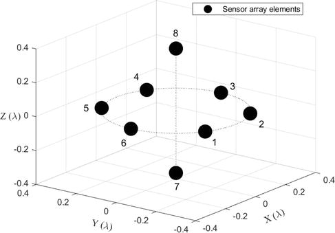
Figure 2.

The spatial positioning of the $M=8$ sensors in 3D UCA configuration. The axes are labeled in wavelengths to provide a scale reference relative to the signal’s wavelength.

This case study details the application of NS for DoA estimation using a 3-D UCA comprising eight sensors ($M=8$). To optimize array performance and prevent grating lobes, the element spacing was set at half the wavelength ($\lambda /2$). The study primarily focuses on the precise estimation of DoAs for two source signals. These signals, at a carrier frequency of 500 MHz, impinge on the array from directions ${\mathtt{\Theta }}_1=\left({30}^{\circ },{60}^{\circ }\right)$ and ${\mathtt{\Theta }}_2=\left({120}^{\circ },{25}^{\circ }\right)$. The simulation process involved 256 snapshots and maintained a signal-to-noise ratio (SNR) of 20 dB to facilitate accurate DoA estimations.

The NS algorithm is initialized with a set of live points drawn from the prior distribution, which, in this case, is uniform over the feasible intervals of azimuth and elevation, given as in (7) and (8), respectively. The simulation iterates over the NS loop, replacing low-likelihood points with new samples (14), until convergence criteria based on the Bayesian evidence Z are met (17).

Figure 3 illustrates a visual representation of our attempt to estimate the DoAs using NS, which successfully estimated the azimuth and elevation of the two signals. The estimated values, represented by the red cross markers on the contour plot, closely match the actual DoAs of the signals, indicated by the green circle markers. This close correspondence between the red and green markers demonstrates the accuracy of NS. In an ideal scenario, the red and green markers would completely overlap, signifying a perfect estimation.

Figure 3.

Parameter estimation using NS for azimuth and elevation. The contour plot shows the posterior distribution of the parameters. The estimated directions of the signals are indicated by red crosses, while green circles depict their actual positions. The histograms show the marginal distributions of the parameters. Dashed red lines represent estimations, whereas solid green lines represent actual positions.

To further assess the accuracy, we analyzed the distribution of estimates using the histograms flanking the contour plot. These histograms, resembling mountain ranges, reveal how frequently estimates fall within specific angular ranges. Essentially, they represent a popularity contest for angles. The left histogram focuses on azimuth angles, while the right histogram deals with elevation angles. In both histograms, we observe peaks indicating the concentrations of estimates, represented by the dashed red lines. The actual signal directions are marked by solid green lines.

Comparing the estimated and actual signal directions, we find that estimates at ${\widehat{\mathtt{\Theta }}}_1=\left({30.9}^{\circ }{\mathrm{,58.89}}^{\circ }\right)$ and ${\widehat{\mathtt{\Theta }}}_2=\left({122.9}^{\circ }{\mathrm{,23.847}}^{\circ }\right)$ are quite close to the true directions of ${\mathtt{\Theta }}_1=\left({30}^{\circ },{60}^{\circ }\right)$ and ${\mathtt{\Theta }}_2=\left({120}^{\circ },{25}^{\circ }\right)$, respectively. The smaller the gap between the red and green lines in the histograms, the more accurate the estimation method has performed.

Overall, the results demonstrate that NS algorithm effectively estimates the azimuth and elevation of the two signals. The close match between estimated and actual signal directions, along with the narrow peaks in the histograms, confirms the accuracy of the method.

5. Conclusion

The application of NS to DoA estimation represents an important advancement in array signal processing. This case study underscored the robustness of NS in the context of multi-source signals, demonstrating its ability to provide highly accurate DoA estimates under conditions of limited snapshots and elevated noise levels. The iterative nature of the algorithm was a highlight, showing consistent convergence to the actual signal sources with notable accuracy.

The results from this study illuminate the potential of NS as a viable alternative to conventional DoA estimation techniques, especially in environments characterized by complex distributions and high-dimensional parameter spaces. The strong alignment between the estimated and the actual signal directions, as depicted in the detailed contour plots and histograms, validates the algorithm’s effectiveness.

Looking ahead, the promise of NS extends to a wider range of signal-processing applications. Its ability to navigate complex posterior distributions and efficiently compute marginal likelihoods suggests its suitability for more sophisticated array configurations and signal-processing tasks. As computing power increases, the intensive computational requirements of NS will become less of a barrier, potentially opening the door to its wider implementation in practical signal-processing scenarios. This investigation lays the groundwork for future research and suggests that, with further refinement and optimization, NS could become an indispensable tool in scientific and engineering fields that rely on signal processing.

Conflict of interest

The authors declare no conflict of interest.

References

- 1.
Skilling J. Nested sampling for general Bayesian computation. Bayesian Analysis. 2006; 1 (4):833-859. DOI: 10.1214/06-BA127 - 2.
Henderson RW, Goggans PM, Cao L. Combined-chain nested sampling for efficient Bayesian model comparison. Digital Signal Processing. 2017; 70 :84-93. Available from:https://www.sciencedirect.com/science/article/pii/S1051200417301719 - 3.
Feroz F, Hobson MP, Bridges M. MultiNest: An efficient and robust Bayesian inference tool for cosmology and particle physics. Monthly Notices of the Royal Astronomical Society. 2009; 398 :1601-1614 - 4.
Veitch J, Raymond V, Farr B, Farr W, Graff P, Vitale S, et al. Parameter estimation for compact binaries with ground-based gravitational-wave observations using the LALInference software library. Physical Review D. 2015; 91 :042003. DOI: 10.1103/PhysRevD.91.042003 - 5.
Higson E, Handley W, Hobson M, Lasenby A. Dynamic nested sampling: An improved algorithm for parameter estimation and evidence calculation. Statistics and Computing. 2019; 29 (5):891-913. DOI: 10.1007/s11222-018-9844-0 - 6.
Van Trees HL. Optimum array processing: Part IV of detection, estimation, and modulation theory. New York: John Wiley & Sons; 2002 - 7.
Schmidt R. Multiple emitter location and signal parameter estimation. IEEE Transactions on Antennas and Propagation. 1986; 34 (3):276-280 - 8.
Roy R, Kailath T. ESPRIT-estimation of signal parameters via rotational invariance techniques. IEEE Transactions on Acoustics, Speech, and Signal Processing. 1989; 37 (7):984-995 - 9.
Feroz F, Hobson MP, Cameron E, Pettitt AN. Importance nested sampling and the MultiNest algorithm. The Open Journal of Astrophysics. 2019; 11 :2 - 10.
Aitken S, Akman OE. Nested sampling for parameter inference in systems biology: Application to an exemplar circadian model. BMC Systems Biology. 2013; 7 (1):72. DOI: 10.1186/1752-0509-7-72 - 11.
Speagle JS. Dynesty: A dynamic nested sampling package for estimating Bayesian posteriors and evidences. Monthly Notices of the Royal Astronomical Society. 2020; 493 (3):3132-3158 - 12.
Buchner J. Nested sampling methods. Statistics Surveys. 2023; 17 :169-215. DOI: 10.1214/23-SS144 - 13.
Tawara N, Ogawa T, Watanabe S, Kobayashi T. Nested Gibbs sampling for mixture-of-mixture model and its application to speaker clustering. APSIPA Transactions on Signal and Information Processing. 2016; 5 :e16 - 14.
Buchner J. Collaborative nested sampling: Big data versus complex physical models. Publications of the Astronomical Society of the Pacific. 2019; 131 (1004):108005. DOI: 10.1088/1538-3873/aae7fc - 15.
Alsing J, Handley W. Nested sampling with any prior you like. Monthly Notices of the Royal Astronomical Society: Letters. 2021; 505 (1):L95-L99 - 16.
Ashton G, Bernstein N, Buchner J, Chen X, Csányi G, Fowlie A, et al. Nested sampling for physical scientists. Nature Reviews Methods Primers. 2022; 2 (1):39. DOI: 10.1038/s43586-022-00121-x - 17.
Vitale S, Del Pozzo W, Li TGF, Van Den Broeck C, Mandel I, Aylott B, et al. Effect of calibration errors on Bayesian parameter estimation for gravitational wave signals from inspiral binary systems in the advanced detectors era. Physical Review D. 2012; 85 :064034. DOI: 10.1103/PhysRevD.85.064034 - 18.
Allison R, Dunkley J. Comparison of sampling techniques for Bayesian parameter estimation. Monthly Notices of the Royal Astronomical Society. 2013; 437 (4):3918-3928. DOI: 10.1093/mnras/stt2190 - 19.
Higson E, Handley W, Hobson M, Lasenby A. Sampling errors in nested sampling parameter estimation. Bayesian Analysis. 2018; 13 (3):873-896. DOI: 10.1214/17-BA1075 - 20.
Thrane E, Talbot C. An introduction to Bayesian inference in gravitational-wave astronomy: Parameter estimation, model selection, and hierarchical models. Publications of the Astronomical Society of Australia. 2019; 36 :e010 - 21.
Paulen R, Gomoescu L, Chachuat B. Nested sampling approach to set-membership estimation. IFAC-Papers OnLine. 2020; 53 (2):7228-7233 21st IFAC World Congress. Available from:https://www.sciencedirect.com/science/article/pii/S2405896320308545 - 22.
Jasa T, Xiang N. Nested sampling applied in Bayesian room-acoustics decay analysisa. The Journal of the Acoustical Society of America. 2012; 132 (5):3251-3262. DOI: 10.1121/1.4754550 - 23.
Fackler CJ, Xiang N, Horoshenkov KV. Bayesian acoustic analysis of multilayer porous media. Journal of the Acoustical Society of America. 2018; 144 (6):3582-3592. Available from:https://eprints.whiterose.ac.uk/141044/ , - 24.
Landschoot CR, Xiang N. Model-based Bayesian direction of arrival analysis for sound sources using a spherical microphone array. The Journal of the Acoustical Society of America. 2019; 146 (6):4936-4946. DOI: 10.1121/1.5138126 - 25.
Krim H, Viberg M. Two decades of array signal processing research: The parametric approach. IEEE Signal Processing Magazine. 1996; 13 (4):67-94 - 26.
Keskin F, Filik T. An optimum volumetric array design approach for both azimuth and elevation isotropic DOA estimation. IEEE Access. 2020; 8 :183903-183912