The Role of Earthquake Catalogue in Seismic Tomography

Abstract

Seismic tomography is a process used to know a structure in the depth of a determined part of Earth. It consists of two parts. The first one, the so-called Forward Problem, provides a computation of theoretical traveltimes starting from an estimate of hypocentral parameters obtained by earthquakes registered by a specific network of seismic stations. The second one, the so-called Inverse Problem, aims at providing a 3-D seismic velocity model obtained minimising residuals, that is the difference between theoretical and observed traveltimes. The production of a well-distributed earthquake catalogue is really important to obtain a well-performed seismic tomography. So, it is relevant to the description of the rules to achieve an acceptable and performing earthquake catalogue for seismic tomography. Three examples are shown: local tomography, regional tomography, teleseismic tomography. In each of them, broad relevance has been given to the theoretical background and to the formation of an earthquake catalogue with just a hint (images only) to the final results.

1. Introduction

Through the word tomography, a process adopted in many known sciences (for example, medicine, oceanography, etc…) has been described. A process with an only aim: studying the internal structure of a determinated system by means of a series of sources that enlighten it. For example, the Computer Axial Tomography (CAT) is used in medicine and consists of X-Ray beams that barrage the body of a person to light up his (or her) internal. Seismic tomography works in the same way. This process allows us to know the principal characteristics of a structure in the depth of a determinated part of Earth. Seismic tomography could be divided into three categories: seismic refraction tomography, attenuation seismic tomography and the “classic” traveltime seismic tomography. For brevity, only the last one will be described in this chapter.

1.1 Traveltime seismic tomography: a general description

A traveltime seismic tomography follows the established model of a so-called Inverse Problem [1]. That is, the following structure is implemented in this way (Figure 1):

Figure 1.

Graphic description of an inverse problem.

Part 1, Forward Problem - Theoretical traveltimes starting from an estimate of hypocentral parameters are computed. This estimate is obtained by a 1-D starting velocity model.

Part 2, Inverse Problem – Estimate of the hypocentral parameters through a comparison between theoretical and observed results.

In this regard, for each datum, the estimate of residual (Eq. (1)) that is the difference between the observed travel times (labelled Tr.time^obs) and these theoretical travel times (labelled Tr.time^teo) takes considerable importance. This is because the entire process stops when the residual touches its minimum value.

$$\mathit{\text{Residuals}}=\mathit{Tr}.{\mathit{\text{time}}}^{\mathit{obs}}-\mathit{Tr}.{\mathit{\text{time}}}^{\mathit{teo}}$$E1

Generally, traveltime seismic tomography is a non-linear problem [2]. A generic travel time Tr.time along a ray r is given by:

$$\mathit{Tr}.\mathit{\text{time}}=\underset{r\left(s\right)}{\int }s\left(r\right)\mathit{ds}$$E2

where s is the slowness, that is the reciprocal of velocity of seismic wave v. Using slowness instead of velocity, we could affirm that (Eq. (2)) is linear. This affirmation is wrong. In fact, rays are curves of stationary travel time and therefore depend on the slowness. So, slowness compares both in the integrand and it determines ray position r(s) in (Eq. (2)). Before proceeding, we should linearize (Eq. (2)). For obtaining this result, Fermat‘s principle has invoked. It says that the travel along a ray does not change to first order when this ray is perturbed. This principle has been applied to the following equation:

$${\left|\nabla \mathit{Tr}.\mathit{\text{time}}\right|}^2=s^{2}r$$E3

It is the eikonal equation, that is an equation which describes the propagation of a wavefront Tr.time and its solution allows us to compute traveltimes. By means of a systematic permutation approach, eikonal equation can be linearized. For solving it, 1-D velocity model has been discretized in a sort of grid (Jeffreys-Bullen model, AK135, IASP91) (Figure 2). In this way, seismic tomography becomes a typical matrix problem solvable by means of specific numerical algorithms (MTTT, difference finite eikonal equation, Fast Marching for the forward problem, least squares for the inverse problem [3]).

Figure 2.

Schematic description of a grid for traveltime seismic tomography. T_i is the i-th traveltime used for the inversion, Δs_i^j is the grid step for T_i traveltime through j-th grid cell, “point” symbolises hypocenter, “triangle” symbolises seismic station.

Performing a seismic tomography obviously has the goal of obtaining good results. A goal can be reached if all the characteristics used for realising a seismic tomography are refined. For example, numerical characteristics (choice of grid limits, grid tests, etc.…), informatics, computing characteristics (capability of computers, software elaboration, software graphic). But one characteristic is fundamental: the assembly of an opportune database of seismic events. Who performs a seismic tomography should answer to following guidelines questions: (1) How many seismic events are needed? (2) By what criteria (magnitude, type, period) seismic events are selected? (3) By what criteria (geometrical distribution, acquisition of a determined seismic event) a network of seismic stations is selected? Relevant questions that have not absolute answers but these last ones could change depending on the geophysical situation. In this proposal, three different situations are shown. That is, a local, a regional and a teleseismic traveltime tomography. Three different situations with the aim of finding a common denominator in the production of a seismic catalogue.

1.2 The example of a local seismic tomography

The first one is a local seismic tomography (that is a seismic tomography of an area almost 100x100 km) of Campania and Basilicata, two regions of South Italy that on 23th of November 1980 were shattered by a disastrous earthquake (M_W = 6.9, 2483 dead people and 7700 injured) [4]. In this case, the seismic catalogue consists of 665 events that are the aftershocks (Figure 3) acquised by the Italian seismological network and temporary seismic network in the period 1–15 December 1980 (107 stations) for a total of 18,625 P phases. Following the guidelines of questions previously mentioned, it is possible to understand that:

Figure 3.

Geographical distribution of aftershocks of Irpinia earthquake (23rd November 1980) used to construct earthquake catalogue for local Irpinia traveltime seismic tomography.

(1) Considering the strong magnitude of mainshock and consequently big number of aftershocks, it seems quite reasonable that two weeks of continuous acquisition are enough for having a complete database; (2) Being a local seismic tomography, it makes little sense to operate a strong selection from point of view of magnitude (except for instrumental earthquakes); (3) a strong set of local seismic station has been chosen with the support of Italian seismological network for having a better geometrical distribution (Figure 4).

Figure 4.

Network of seismic stations for local Irpinia traveltime seismic tomography.

An image of a horizontal section of local Irpinia tomography is shown (Figure 5).

Figure 5.

Horizontal section of Irpina local tomography at 3 km depth.

1.3 The example of a regional seismic tomography

The second one is a regional seismic tomography of circum-arctic [5]. That is, a tomography with a database composed of earthquakes whose epicentral distance is included in the range [100 km; 1400 km]. In this way, whereas the epicentral distance is greater than the similar one in local earthquakes, seismic rays could “illuminate” a higher depth. For producing an optimal database, in these cases, a database of the International Seismic Centre (ISC) is used. It is a database consisting of 4 million seismic events, not only earthquakes but also artificial explosions and a network of even 50 million individual seismic stations.

In this regional seismic tomography of circum-arctic (Figure 6), P waves of local earthquakes recorded by ISC seismic stations (number not specified) at a regional distance in a period [1964–2007] are used for producing the database (Figure 7).

Figure 6.

Topographic/bathymetric map of Circum-arctic region.

Figure 7.

Distribution of seismic events and seismic stations in circum arctic region. Red dots represent ISC seismic events, blue triangles are seismic stations.

Grid for tomography is 7000 x 7000 x 50 km in depth, with a maximum depth of 640 km (that is, near at range of maximum depth at which an earthquake can occur, 660–700 km in the lower mantle). In this work, more inversions have been performed at different orientations and their average in one model has been considered. The distribution of events and the seismic station is very irregular for the simple reason that in the central part of the circum-arctic region there are not seismic stations and consequently there is very poor ray coverage. Answering the “guideline questions”, it is possible to notice:

(1) The huge number of seismic events and making recourse to the ISC seismic catalogue represent an obvious choice because of the goal of tomography (that is, the study of greater depths); (2) The huge number of data is strictly connected with the risk of poor quality. Indeed, a preprocessing and a selection of data by means of determined (but not specified) criteria has been performed; (3) Considering the geographical peculiarity of the zone, even in this case the choice of network stations is obliged.

Images of horizontal sections of regional Circum-Arctic tomography have been shown (Figure 8).

Figure 8.

Distribution of seismic events and seismic stations in Circum-arctic region. Red dots represent ISC seismic events, blue triangles are seismic stations.

1.4 The example of a teleseismic tomography

The third and last (but not the least) case is a teleseismic tomography of Southern Tyrrhenian [6, 7]. Teleseisms are earthquakes whose epicentral distance (expressed in angular distance) is greater than 30°(Figure 9). The Tyrrhenian Sea is a back-arc basin (that is, it is a basin made up of oceanic crust associated with a roll-back subduction that is a result of the subducting Ionian slab since the Tortonian Age (10 Ma) [8]. At the present day, most of the oceanic lithosphere in the Tyrrhenian-Apennine system has been consumed with the exception of the 74 Calabrian arc sector where there is still subducting Ionian lithosphere, confined to the southwest by the Malta Escarpment [9].

Figure 9.

Graphical representation of a comparison between local and teleseismic earthquake.

Teleseismic tomography has been chosen because the 3D models obtained only to describe in a good way the crust and the first part of the upper mantle (maximum reached depth of Southern Tyrrhenian local tomographies is 350 km) and in scientific literature there are few works of teleseismic tomography regarding Southern Tyrrhenian [10].

The used database consists of 2979 teleseisms recorded (Figure 10) by 285 Italian ISC seismic stations (Figure 11) from 1980 to 2012 with a total of 18,515 arrival times relating to P phases. For obtaining a better stability, a preprocessing of data has been performed by means of the following criteria:

• magnitude >6

• epicentral distance included in the range [20°; 100°]

• station residual included in the range [−2 seconds; 2 seconds]

• each teleseism must be recorded by almost 10 stations

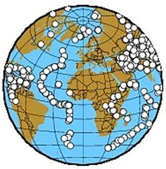
Figure 10.

Map of events (white dots) for southern Tyrrhenian teleseismic tomography.

Figure 11.

Map of ISC seismic stations (white triangles) for southern Tyrrhenian teleseismic tomography.

The distribution of the seismic station is coherent with the area object of tomographic investigation because ISC Southern Italy has been chosen. Grid for tomography has been constructed following these criteria: 0–500 km in depth; 7°-20° E in longitude; 35°-48° N in latitude while grid spacing is 50 km in depth; 0.8 degrees in longitude, 0.4 degrees in latitude (Figures 12 and 13). Answering three guidelines questions: (1) Being (fortunately) teleseisms seismic events not very common, it seemed very reasonable that a very large period (32 years) was considered; (2) Chosen criteria of preprocessing data have been established to obtain data uniformity; (3) For obtaining a good ray coverage in the tomographic area, it seemed very reasonable, considering their availability, the choice of all available ISC Southern Italy seismic stations.

Figure 12.

Horizontal section of southern Tyrrhenian teleseismic tomography at 50 km depth.

Figure 13.

Horizontal section of southern Tyrrhenian teleseismic tomography at 250 km depth.

2. Conclusions

The topic of this chapter concerns the role of the formation of a seismic catalogue for performing a traveltime tomography. Three several typologies have been shown: a local, a regional and a teleseismic one.

For all typologies, the seismic catalogue is composed of P seismic phases. This is because of the stability of this phase and the overall presence and easiness of picking on a seismogram. The strong differences among these typologies of tomographies regard the formation of the database, above all in number and period of acquisition of events, choice of seismic stations and their geometrical distribution in the area of investigation.

As regards local tomography – that has as its goal the “illumination” of shallow depths - it seems reasonable that the construction of a database composed of seismic events in the hundreds acquised by a network of seismic stations. The geometrical distribution of these last ones is simply the current network of seismic stations in the area of investigation. A more stable case for local tomography is (as in the case of example) when seismic events are aftershocks of a main event. This is for two reasons: 1) a practical reason because in a few days, the construction of the database has been performed; 2) a “scientific” reason because the magnitude of aftershocks is more or less similar, therefore there is a major uniformity and sturdiness of data.

As regards regional and teleseismic tomography, making recourse to the ISC catalogue is almost obliged because regional and teleseismic events could be acquised by local seismic stations but in lots of situations their archives are not rich events in enough number for performing a tomography. This choice implicates two consequences: 1) the construction of a database for a period of almost 30–40 years; 2) the development of “a priori” conditions to select data for performing a sort of “data preprocessing” in such a way the used data are “clean” and ready to be analysed for a tomography. In this way, the number of data is one-two order of magnitude greater than its equivalent for the local one.

Regarding the network of seismic stations, local tomography establishes the restriction to use a network of local seismic stations geometrically distributed in the area of investigation in a uniform way while the use of ISC seismic catalogue offers more freedom of choice, although the use of seismic stations located in the area of investigation is more advisable.

Therefore, a construction of a correct seismic catalogue is a necessary (but not sufficient) condition to perform an optimal traveltime seismic tomography.

References

- 1.
Tarantola A. Inverse Problem Theory: Methods for Data Fitting and Model Parameter Estimation. Amsterdam: Elsevier; 1987 ISBN: 0898715725 - 2.
Nolet G. Seismic wave propagation and seismic tomography. In: Nolet G, editor. Seismic Tomography. Seismology and Exploration Geophysics. Vol. 5. Dordrecht: Springer; 1987. DOI: 10.1007/978-94-009-3899-1_1 - 3.
Paige CC, Saunders MA. LSQR: An algorithm for sparse linear equations and sparse least squares. ACM Transactions on Mathematical Software. 1982; 8 (1):43-71. DOI: 10.1145/355993.356000 - 4.
Pucciarelli G. Tomographic Inversion of Data Acquised by Aftershocks in Period 1–15 December 1980 of the Campano-Lucano Earthquake, 23th Novembre 1980. University of Salerno, Dept of Physics; 2009. DOI: 10.14273/unisa-968 - 5.
Yakovlev AV, Bushenkova NA, Yu KI, Dobretsov NL. Structure of the upper mantle in the Circum-arctic region from regional seismic tomography. Russian Geology and Geophysics. 2012; 53 :963-971. DOI: 10.1016/j.rgg.2012.08.001 - 6.
Pucciarelli G. Seismic Tomography of Southern Tyrrhenian by Means of Teleseismic Data. University of Salerno, Dept of Physics; 2017. DOI: 10.14273/unisa-968 - 7.
Pucciarelli G. Seismic tomography of southern Tyrrhenian by means of teleseismic data. In: Proceedings of GNGTS 38th National Congress. Rome: University of Salerno, Dept of Physics; 12–14 November 2019. DOI: 10.13140/RG.2.2.14144.89609 - 8.
Chiarabba C, De Gori P, Speranza F. The southern Tyrrhenian subduction zone: Deep geometry, magmatism and Plio-Pleistocene evolution. Earth and Planetary Science Letters. 2008; 268 :408-423. DOI: 10.1016/j.epsl.2008.01.036 - 9.
Calò M, Dorbath C, Luzio D, Rotolo SG, D’Anna G. Seismic velocity structures of southern Italy from tomographic imaging of Ionian slab and petrological inferences. Geophysical Journal International. 2012; 191 (2):751-764. DOI: 10.1111/j.1365-246X.2012.05647.x - 10.
Montuori C, Cimini GB, Favali P. Teleseismic tomography of the southern Tyrrhenian subduction zone: New results from seafloor and land recordings. Journal of Geophysical Research. 2007; 112 (B03311):2007. DOI: 10.1029/2005JB004114