Comparison of Site Response Analysis (SRA) According to Ground Modelling and Structure Consideration

Abstract

When an earthquake occurs, the seismic motion is amplified as it passes through the ground layers. In addition, even for the same earthquake, the magnitude of the ground response on the ground surface varies depending on the ground condition. Determining the response within the ground following an earthquake is called site response analysis (SRA), and a general standard procedure is to perform site response analysis using the 1D (one-dimensional) wave propagation theory. However, in the case of one-dimensional site response analysis, complex topography, ground surface changes, and effects on structures are not included. Therefore, evaluating the reasonable ground response that may occur in the actual field is necessary. This article analyses ground amplification phenomena according to modelling differences through 2D (two-dimensional) and 3D (three-dimensional) modelling that can consider complex topography in addition to 1D. In addition, the nonlinear characteristics of the soil and the interaction between the soil and the structure were considered, and time history analysis was performed to identify the realistic dynamic behaviour characteristics of the soil and structure.

1. Introduction

The amplitude and frequency characteristics of seismic waves propagated through bedrock change depending on the characteristics of the ground they pass through until they reach the surface. In the case of vibration characteristics, it is affected by various causes such as earthquake magnitude, distance to the epicentre, duration, and site support characteristics.

When examining past earthquake records, despite the same earthquake, different seismic accelerations occurred on the ground surface where the structure was located depending on the ground conditions, and the extent of the resulting damage was also different. Therefore, the dynamic response of a structure during an earthquake is determined by the composition of the ground supporting the structure. Therefore, Site Response Analysis (SRA), which analyzes the amplification in the ground when an earthquake occurs, is the first step and an essential factor in evaluating the stability of a structure caused by the earthquake.

The SRA is an important factor that determines the dynamic characteristics of a structure, and various studies have been conducted on the reliability of the analysis. In the early stage of the study, due to the limitation of computer performance, the reliability study of equivalent linear analysis with simple input variables and short analysis time was the main focus. A representative study verifies the recorded motion of the rock outcrop and ground surface free field of the Northridge earthquake that occurred in Los Angeles, USA [1]. However, recent studies are focused on the lack of reliability of the results of equivalent linear analysis when the complex ground layer shape and surface cannot be considered, and the shear strain is significant. Therefore, various methods have been studied to solve these disadvantages, and various analysis methods and software have been developed for this purpose.

In this article, the Hardening soil in small strain material model, which is a non-linear model that can more accurately consider the deformation of the soil, was applied. And the ground was modelled in 1D, 2D, and 3D to compare the ground response results according to modelling changes. In addition, the structure was modelled in 2D and 3D models that can consider the structure, and the results of the site response were compared.

2. Site response analysis (SRA)

Site Response Analysis, also called free-field analysis, refers to a method and process for obtaining the response within the ground to a given seismic input in the unexcavated ground state before the structure is built when the location to be constructed is determined (Figure 1) [2].

Figure 1.

Schematic representation of site response analysis.

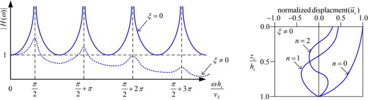
Generally, 1D equivalent linear analysis, which is relatively simpler than other analysis methods, is widely used for SRA. This assumes that all soil layers are elastic halfspace horizontal bodies without separately modelling the soil layer, so it is assumed that the response of the ground is affected only by shear waves propagating vertically from the bedrock [3]. It can be expressed as the amplification function $A\left(\omega \right)$ when a shear wave is incident perpendicular to the fault elastic ground laid horizontally on the elastic rock halfspace.

$$A\left(\omega \right)=\left|H\left(\omega \right)\right|=\left|\frac{U\left(0,\omega \right)}{U\left(h_s,\omega \right)}\right|=\frac{1}{\left|cos\left(\frac{\omega h_s}{V_s}\right)\right|}\ge 1$$E1

Where $H\left(\omega \right)$ is the complex transfer function, $U\left(z,\omega \right)$ is the magnitude of horizontal displacement at depth, $\omega$ is angular frequency, $h_s$ is the depth, and $V_s$ is shear-wave velocity of the soil layer. For $\frac{\omega h_s}{V_s}=\frac{\pi }{2}+\mathit{n\pi }$, with $n=0,1,2,3\dots$, the amplification function has a tendency to infinity, which means resonance. Here, when $n$= 0, $\omega$ is equal to the natural or fundamental frequency of the layer and is calculated as follows.

$${\omega }_n=\frac{\pi V_s}{2h_s},{\mathrm{ƒ}}_n=\frac{V_s}{4h_s}$$E2

The amplification function can be modified to account for the effect of energy dissipation in the soil. A straightforward approach is to assume that the material damping is viscous. Applying damping means that the displacement amplitude associated with the resonant frequency is no longer infinite, and Eq. (1) is modified by [2].

$$A^{\ast }\left(\omega \right)=\left|H^{\ast }\left(\omega \right)\right|=\frac{1}{\sqrt{{\mathit{cos}}^2\left(k{h}_s\right)+{\left(\xi k{h}_s\right)}^2}}$$E3

where $\kappa$ is the wave number and is the $\xi$ damping ratio.

As mentioned above, in the case of 1D equivalent linear analysis, it is assumed that the ground is an elastic halfspace of horizontal material, so it cannot reasonably consider irregular strata or surface topography. In the case of a valley or basin ground shape with accumulated sediments, complex waves can be generated due to multiple refraction and reflection effects of seismic waves, leading to long-duration ground motions and high amplification [4]. Therefore, in this case, appropriate ground shapes should be considered through 2D and 3D model applications according to the site shape (Figure 2).

Figure 2.

Complex transfer functions and mode shapes of fault soils on bedrock [5].

As such, 2D and 3D model evaluations must be performed to properly apply the irregular strata or topography of the actual site. However, going from one dimension to the next involves several problems. First, it is impossible to construct a 2D shape that perfectly matches the dynamic motion of an actual 3D shape [6]. In addition, it is known that 2D models with the same dimensions and material properties generally overestimate the dynamic stiffness and radiation damping of soil due to geometric wave diffusion [2].

When a structure is built on soft ground, the seismic wave characteristics at the bottom of the foundation vary depending on the shape and characteristics of the structure. Therefore, the seismic behaviour of a structure built on soft ground also differs significantly from that built on bedrock [7].

3. Hardening soil (HS) model

Schanz et al. [8] designed the Hardening Soil (HS) model to reproduce basic soil macroscopic phenomena such as soil densification, stress-dependent stiffness, plastic yielding, etc. Unlike other models, such as the Cap model or the Modified Cam Clay (as well as the Mohr-Coulomb model), the magnitude of soil deformation can be more accurately modelled by incorporating three input stiffness parameters corresponding to the triaxial loading stiffness (E₅₀), the triaxial unloading-reloading stiffness (E_ur) and the oedometer loading factor (E_oed) (Figure 3) [9, 10].

Figure 3.

Hyperbolic stress-strain relationship.

4. Analysis conditions

For numerical analysis, PLAXIS software developed by Bentley Systems was used, and in the case of PLAXIS, various ground material models are loaded, enabling various deformation analyses of the ground. In addition, it is possible to simulate complex ground deformation, such as dynamic analysis by earthquake load.

This article studies the effect of ground amplification on modelling changes according to 1D, 2D, and 3D for the same ground condition during an earthquake. In addition, in 2D and 3D analysis, the effect of the structure on ground amplification is compared by applying the structure.

4.1 Element dimension

In dynamic analysis, an element’s size is an important consideration. Unlike 1D modelling, which only considers height, 2D and 3D modelling must also consider width and depth. Discretizing the space is very important because the wave propagation in the continuum must be modelled in 2D or 3D. If the element size in the finite element analysis is too large, the results for high-frequency bands are inaccurate, and if the element size is too small, the results may appear unstable [11].

Therefore, to reduce this error, the maximum frequency transmitted by the analytical model can be estimated based on the largest element or zones within the slowest material, as shown in the following Eq. [6, 12].

$$△l_{\mathit{max}}\le \frac{{\lambda }_{\mathit{min}}}{10}\le \frac{V_{s,\mathit{min}}}{10{\mathrm{ƒ}}_{\mathit{max}}}\mathit{\text{or}}{\mathrm{ƒ}}_{\mathit{max}}\le \frac{V_{s,\mathit{min}}}{10∆{\lambda }_{\mathit{max}}}$$E4

where $△l_{\mathit{max}}$ is the maximum dimension of the element, $\lambda$ the wavelength of the passing wave, $V_s$ is the layer’s shear-wave velocity and ${\mathrm{ƒ}}_{\mathit{max}}$ is the maximum frequency of interest, which is typically around 10 to 15 Hz.

4.2 Boundary

Dynamic analysis using the finite element method, various ground boundary conditions can be applied. In particular, if the boundary conditions are not adequately established in the numerical analysis modelling process during dynamic analysis, correct results may not be derived because the input earthquake may be reflected from the modelling boundary conditions and may occur larger than the actual ground deformation due to the earthquake. Therefore, the boundary condition can be applied by dividing the bottom and side parts. The bottom part applied a compliant base (infinite boundary), and the side part was used with free-field conditions.

4.3 Input ground motions

Time-history analysis was applied for SRA, and determining the input seismic wave at this time is essential in securing the reliability of analysis and evaluation. Therefore, for seismic design, it is necessary to reflect the characteristics of the area where the structure is located and, at the same time, satisfy the design standards suitable for the level of the structure. However, in this analysis, since the effect on ground amplification is the main concern, Koyna and Nahanni earthquakes with different frequency characteristics were used to increase the reliability of the analysis (Figure 4).

Figure 4.

Time history and fast Fourier transfer of (a) Koyna and (b) Nahanni earthquake record.

The Koyna earthquake occurred in 1967 near Koynanagar town in Maharashtra, India. The magnitude 6.6 shock hit with a maximum Mercalli intensity of VIII. The Koyna earthquake is believed to be triggered by a fluid pressure change due to the reservoir’s water percolation into the subsurface [13].

The Nahanni earthquake occurred in 1985 in the Nahanni region of the Northwest Territories, Canada. The magnitude 6.9 shock hit with a maximum Mercalli intensity of VI. The Nahanni earthquakes mainly occurred along fault planes, so fault activity is known as the leading cause of earthquakes [14].

The Peak Ground Acceleration (PGA) of the Koyna earthquake recorded is 3.35 m/s² (0.34 g), and the characteristics of the frequency of the Koyna earthquake through the Fourier transform are confirmed to have frequency components in various intervals from 2.5 to 10 Hz. The PGA of the Nahanni earthquake recorded is 4.80 m/s² (0.49 g), and the frequency characteristics of 2.0 to 3.0 Hz are confirmed.

In the case of the Koyna earthquake, the PGA is lower than that of the Nahanni earthquake, but the frequency range is wide, and the shorter period characteristic is more significant than that of the Nahanni earthquake. In the case of the Nahanni earthquake, the PGA is significant, but the frequency is characterised by a long period. Through the characteristics of these different earthquakes, we tried to secure the reliability of the analysis by considering the effects of the other natural frequencies of the structure and the ground.

4.4 Damping

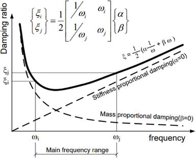
According to the Rayleigh damping formula, the damping matrix $C$ is a linear sum of the mass matrix $M$ and the stiffness matrix $K$ as a function of the Rayleigh coefficients α and β.

$$\left[C\right]=\alpha \left[M\right]+\beta \left[K\right]$$E5

Here, α and β are proportional constants between mass and stiffness, and the relationship between the natural frequency and the damping ratio for the nth mode is as follows.

$${\xi }_n=\frac{1}{2}\left(\alpha \frac{1}{{\omega }_n}+\beta {\omega }_n\right)$$E6

If the damping ratios for the ith and jth modes, which are the two main modes, are ξ_i and ξ_j, α and β can obtain the following simultaneous equations.

$$\approx \left\{\begin{array}{c}{\xi }_i\\ {\xi }_j\end{array}\right\}=\frac{1}{2}\left[\begin{array}{cc}1/{\omega }_i& {\omega }_i\\ 1/{\omega }_j& {\omega }_j\end{array}\right]\left\{\begin{array}{c}\alpha \\ \beta \end{array}\right\}\to \left\{\begin{array}{c}\alpha \\ \beta \end{array}\right\}=\frac{2{\omega }_i{\omega }_j}{{\omega }_j^2-{\omega }_i^2}\left[\begin{array}{cc}{\omega }_j& -{\omega }_i\\ -1/{\omega }_j& 1/{\omega }_i\end{array}\right]\left\{\begin{array}{c}{\xi }_i\\ {\xi }_j\end{array}\right\}$$E7

Such damping is called Rayleigh damping, and the damping matrix at this time is called a Rayleigh damping matrix or a proportional damping matrix.

In applying Rayleigh damping, it is important to note that the two modes (ith and jth modes) must be properly calculated to guarantee a reasonable damping ratio for all vibration modes contributing to the response (Table 1).

	ξ (%)	${ƒ}_1$ (or ${\omega }_1$) (Hz)	${ƒ}_2$ (or ${\omega }_2$) (Hz)	α	β
Structure	2.0	0.840	3.862	0.1734	0.0014
Soil	5.0	0.778	0.816	0.2502	0.0099

Table 1.

Input value of Rayleigh damping.

4.5 Materials

In the case of soil material models, the most widely used model is the Mohr-Coulomb (MC) failure model. Numerical analysis is also widely used because the input parameters are more straightforward than other material models [15]. Therefore, the MC model is suitable for failure with large shear deformation during the collapse and is mainly used for stability analysis of dams, slopes, embankments, and shallow foundations [14]. However, in the case of the MC model, it is not easy to reasonably reflect other ground behaviour conditions during loading and unloading.

The Hardening Soil model was developed to more accurately reflect the ground behaviour by supplementing the disadvantages of the MC model. Among them, in the case of Hardening Soil in Small Strain, accurate simulation is possible in evaluating ground amplification caused by earthquakes (Table 2).

	Set1 (limestone)	Set2 (sand)	Set3 (clay)	Set4 (sand)	Set5 (silt)	Set6 (fill)
$E_{50}^{\mathit{ref}}$ (kN/m^2); Secant stiffness in standard drained triaxial test	190,000	75,000	15,000	8500	8500	10,000
$E_{\mathit{oed}}^{\mathit{ref}}$ (kN/m^2); Tangent stiffness for primary oedometer loading	190,000	75,000	15,000	6150	6000	10,000
$E_{\mathit{ur}}^{\mathit{ref}}$ (kN/m^2); Unloading/reloading stiffness	575,000	300,000	50,000	25,750	23,000	30,000
M (−); Power for stress-level dependency stiffness	0.3	0.55	0.7	0.7	0.9	0.5
$c^{\prime }$ (kN/m^2); Cohesion	200	1	25	6	30	10
${\varnothing }^{\prime }$ (°); Friction angle	35	38	20	28	32	25
${\psi }^{\prime }$ (°); Dilatancy angle	0	6	0	6	10	0
${\nu }_{\mathit{ur}}$ (−); Poisson’s ratio for unloading/reloading	0.2	0.2	0.15	0.29	0.3	0.2
$K_0^{\mathit{NC}}$ (−); K0-value for normal consolidation	0.43	0.38	0.66	0.8	0.8	0.58
$G_0^{\mathit{ref}}$ (kN/m^2); Reference value of the shear strain	1,000,000	281,250	90,000	59,883	53,076	50,000
${\gamma }_{0.7}$ (−); Shear strain at which Gs = 0.722G0	0.00005	0.0002	0.00025	0.0003	0.003	0.0002
Υ (kN/m^3); Soil unit weight	23.0	19.0	19.0	18.5	18.5	20.0
$E_s$ (kN/m^2); Soil Elastic modulus	1,040,000	277,000	151,400	150,900	139,100	89,480

Table 2.

Soil model parameters for hardening soil model with small strain [16].

The structure was concrete, and a linear material model was used (Table 3).

	Foundation	Column	Wall
$E$ (kN/m^2)/Elastic modulus	35.16 × 10^6 (35,160 MPa)
Υ (kN/m^3)/Unit weight	25.0
$\nu$ (−)/Poisson’s ratio	0.2
A (m^2)/Area	0.75	0.28	0.30

Table 3.

Structure material parameters.

In Figure 5, the shear-wave velocity according to each layer of the ground is to be evaluated, and the average shear-wave velocity of the entire ground can be confirmed. This soil profile belongs to site class ‘D’ as per the classification of ASCE/SEI 7-10 (Figure 6) [18].

Figure 5.

Rayleigh damping [4].

Figure 6.

Soil and shear-wave velocity profiles [17].

The following is figure about the ground and structures applied to 2D and 3D numerical analysis. The 2D model is mainly used as a plane stress or plane strain model and has the advantage of less analysis time and fewer errors because it is simpler than 3D modelling. However, since the 2D model can be applied only when the evaluation target satisfies the model conditions, 3D model analysis is often required to evaluate the actual site’s response accurately.

To maintain the same conditions as possible with the 2D model during 3D modelling, the aspect ratio of the structure was set to 1:4. When applying an X-direction earthquake, it was modelled to behave in one direction like the 2D analysis (Figure 7).

Figure 7.

Ground layer information in 2D and 3D analysis models.

4.6 Case study

In this article, the analysis is modelled in 1D, 2D and 3D to check the effect of ground amplification according to dimension. Therefore, modelling was conducted for each dimension to confirm this effect, and a sufficient distance was placed in the evaluation area to minimise the effect of boundary conditions (Figure 8).

Figure 8.

Finite element analysis mesh without structure (a) 1D, (b) 2D, and (c) 3D [18].

In addition, an evaluation considering the structure was performed to find out the effect of the structure on the site response amplification (Figure 9).

Figure 9.

Finite element analysis mesh with structure (a) 2D and (b) 3D.

5. Results

When an earthquake occurs, dynamic motion amplifies depending on the ground, and even for the same earthquake, the magnitude of the ground response on the surface varies depending on the consist of the ground. In this article, 2D and 3D modelling, including a basic 1D model, was performed for the same ground to simulate such ground conditions, and an analysis of ground dynamic motion amplification was conducted using PLAXIS software. In addition, modelling a structure in the centre of the ground, an analysis of the amplification change of the ground dynamic motion was also conducted when the structure was considered.

5.1 Site response result according to modelling dimension

The following results from peak ground response acceleration in each stratum according to the difference between 1D, 2D, and 3D models. As a result of the analysis showed very similar peak acceleration results for both Koyna and Nahanni earthquakes in 1D and 2D models. However, in the case of the 3D model, a difference of up to 24% occurred in the case of the Koyna earthquake, and a difference in maximum acceleration of 16% appeared on the surface. In addition, Nahanni earthquake results also showed a difference in peak acceleration of up to 43% and 23% on the surface (Figure 10).

Figure 10.

Peak acceleration results of each dimension by the depth (a) Koyna and (b) Nahanni.

As a result of 1D, 2D, and 3D analysis, the maximum acceleration occurred at the bottom level (−)57.0 m, which is Limestone (Set 1) for both Koyna and Nahanni seismic waves. In general, peak acceleration up to Sand (Set 4) tends to decrease, and then it tends to increase up to the ground surface.

In the soil profile applied to this analysis, the maximum acceleration occurs at the point where the earthquake is input, and no section amplified than the maximum acceleration of the input earthquake is generated within the soil.

For the ground surface, which is the location where the structure is installed and is the most important in ground response, the acceleration according to the time and response spectrum was also reviewed, and the change in peak acceleration according to the periods was also examined.

In the response spectrum results, the 3D model results showed a slightly different tendency from the rest of the analysis results. Overall, a higher response acceleration occurred in the 3D model results over the entire period.

As a result of the response spectrum, the maximum acceleration occurred when the period of the structure was 0.51 sec (1.96 Hz) in the Koyna earthquake, and the maximum difference in the magnitude of the acceleration occurred by 44%. In the Nahanni earthquake, when the period of the structure was 0.55 seconds (1.82 Hz), the magnitude of the acceleration showed a difference of up to 31% (Figure 11).

Figure 11.

Acceleration according to time and response spectrum results (a) Koyna and (b) Nahanni.

5.2 Site response change according to structure consideration

In the 2D model, ground amplification results according to the consideration of the structure resulted in a maximum amplification difference of 12% and 22%, respectively, in the case of maximum acceleration in the two earthquakes. In the case of the Koyna earthquake, the maximum acceleration at the surface was 2% depending on the presence or absence of structures, and the difference in amplification was not significant, but in the case of the Nahanni earthquake, a substantial difference of 22% occurred. In addition, the acceleration results tendency according to the surface’s time was similar for both earthquakes.

However, in the case of response acceleration according to the period in the surface layer, the maximum response acceleration when applied to structures was reduced by 47% in the case of the Koyna earthquake and by 43% in the case of the Nahanni earthquake (Figure 12).

Figure 12.

Peak acceleration by depth, acceleration according to time and response spectrum results in the 2D model with or without structure (a) Koyna and (b) Nahanni.

In the 3D model, the result of ground amplification according to the consideration of the structure showed that both earthquakes had the maximum acceleration difference in the ground surface and were amplified by 10 and 17%, respectively, when the structure was considered. In the 2D results, the maximum acceleration of the surface when the structure was considered was smaller than when the structure was not considered. The acceleration results over time showed similar trends for both earthquakes regardless of whether structures were considered. Despite the significant difference in the maximum response acceleration according to the period in the surface layer, the maximum response acceleration decreased by 5% in the Koyna earthquake and only 2% in the Nahanni earthquake when the structure was installed (Figure 13).

Figure 13.

Peak acceleration by depth, acceleration according to time and response spectrum results in the 3D model with or without structure (a) Koyna and (b) Nahanni.

The following results from the shear stress-strain for each earthquake according to depth. Since the closer to the ground surface, the greater the effect of the structure, the shear stress-strain result also showed a more significant difference in the result with or without structure the closer to the ground surface.

In the case of the Koyna earthquake, a more considerable shear strain occurred than the result of the Nahanni earthquake. Depending on the depth, a difference in shear strain of up to about 10 times occurred, and a significant decrease in shear stiffness was confirmed in the Koyna results compared to Nahanni earthquake (Figure 14).

Figure 14.

Depending on the depth, the shear stress-strain hysteresis curve of results in the 3D model with or without structure (a) Koyna and (b) Nahanni.

In the case of the Koyna earthquake, it is possible to check the strain hardening section due to the generation of max shear strain greater than that of the Nahanni earthquake. In addition, the difference in ground acceleration according to with or without the structure is considered to occur more in Nahanni than in the Koyna earthquake. However, shear strain showed a more significant difference in Koyna than in Nahanni.

That is, even in the same soil condition, the peak acceleration and shear strain occurring in the ground can vary greatly depending on the characteristics of the earthquake.

6. Conclusions

Ground amplification during an earthquake must be identified to determine the design response spectrum, liquefaction evaluation, and seismic load applied to the structure required for the seismic design of the structure. And since SRA is essential to predict this, it can be said that securing the reliability of the analysis is the most important thing.

Therefore, SRA was performed under several conditions in this article, and the following conclusions were obtained.

1. Regarding site response analysis considering only the ground, a significant difference occurred in the 3D analysis result from other results. In 1D and 2D models, vibration occurs only in the X direction, when is the direction in which the earthquake is applied, but in 3D analysis, vibration occurs in the Y direction even if the direction of the earthquake is in the X direction. In addition, SRA using a 3D model requires additional boundary conditions than other models, and since the Rayleigh damping value changes according to the range of the frequency during nonlinear analysis, it is judged that these differences gather and cause a large difference in the result value.

2. In the SRA considering the structure, if the vibration occurs due to the earthquake, inertial force is generated in the structure due to these vibrations. The forces transmitted to the structure in this way are dissipated through the foundation ground again in wave energy. In this analysis result, a significant difference in acceleration amplification was shown depending on whether or not a structure was considered in the response spectrum result of the 2D. In addition, it was found that the characteristics of the response spectrum showed an amplification effect in the low-frequency band compared to the case where the interaction between the ground and the structure was considered. In other words, when the structure was not considered, the ground amplified significantly.

3. Different results from the peak acceleration result were shown in the case of the shear strain occurring in the ground. In the case of the maximum ground acceleration, depending on whether or not the structure was considered, a larger difference occurred in the Nahanni than in the Koyna earthquake, but in the case of shear strain, on the contrary, a large difference was shown in the Koyna earthquake. Therefore, it is necessary to analyse the response amplification of the ground considering various earthquake records.

In conclusion, a larger acceleration amplification occurred when the 3D model was used than other results. Therefore, in the case of SRA using a 3D model, additional analysis of factors that can affect the response results, such as boundary conditions and Rayleigh damping, is required to analyse the differences from other analysis models.

References

1.Idriss IM. Assessment of Site Response Analysis Procedures. U.S Department of Commerce. NIST GCR 95-667; 2000
2.Wolf JP. Dynamic Soil-Structure Interaction. United States: Prentice Hall; 1985
3.Kramer SL. Geotechnical Earthquake Engineering. United States: Prentice Hall; 1996
4.Kuhlemeyer RL, Lysmer J. Finite element method accuracy for wave propagation problems. Journal of the Soil Mechanics and Foundations Division. 1973;99(SM5):421-427
5.Kim DK. Dynamics structures. South Korea: Goomibook; 2013
6.Volpini C, Douglas J, Nielsen AH. Guidance on conducting 2D linear viscoelastic site response analysis using a finite element code. Journal of Earthquake Engineering. 2019;25(4):1-18. DOI: 10.1080/13632469.2019.1568931
7.Rizos DC, Stehmeyer EH. Simplified seismic analysis of soil-foundationstructure systems including soil-structure interaction effects. In: 13th World Conference on Earthquake Engineering. Canada. 2004
8.Schanz T, Vermeer P, Bonier P. Formulation and verification of the Hardening Soil model. In: Beyond 2000 in Computational Geotechnics. 1999
9.Obrzud RF, Truty A. The Hardening Soil Model: A Practical Guidebook. Switzerland: Zace Services; 2010
10.Obrzud RF. On the Use of the Hardening Soil Small Strain Model in Geotechnical Practice. Switzerland: Elmepress International; 2010
11.Saenger EH, Gold N, Shapiro SA. Modeling the propagation of elastic waves using a modified finite-difference grid. Wave Motion. 2000;31(1):77-92
12.Flores Lopez FA, Ayes Zamudio JC, Vargas Moreno CO, Vázquez Vázque A. Site response analysis (SRA): A practical comparison among different dimensional approaches. In: 15th Pan-American Conference on Soil Mechanics and Geotechnical Engineering. Mexico. 2015. DOI: 10.3233/978-1-61499-603-3-1041
13.Das D, Mallik J. Koyna earthquakes: A review of the mechanisms of reservoir-triggered seismicity and slip tendency analysis of subsurface faults. Acta Geophysica. 2020;68:1097-1112
14.Rock and Roll in the N.W.T. The 1985 Nahanni Earthquakes [Internet]. 2021. Available from: https://www.earthquakescanada.nrcan.gc.ca/historic-historique/events/19851223-en.php [Accessed: August 31, 2023]
15.Semet ÇELİK. Comparison of Mohr-coulomb and hardening soil models’ numerical estimation of ground surface settlement caused by Tunneling. Iğdır Üniversitesi Fen Bilimleri Enstitüsü Dergisi. / Igdir University Journal of the Institute of Science and Technology. 2017;7(4):95-102. DOI: 10.21597/jist.2017.202
16.Zhao C, Schmudderich C, Barciaga T, Rochter L. Response of building to shallow tunnel excavation in different types of soil. Computers and Geotechnics. 2019;2019:4. DOI: 10.1016/j.compgeo.2019.103165
17.Nautiyal P, Raj D, Bharathi M, Dubey R. Ground response analysis: Comparison of 1D, 2D and 3D approach. Singapore: Springer; May 2021. DOI: 10.1007/978-981-33-6564-3_51
18.American Society of Civil Engineers. Minimum Design Loads for Buildings and Other Structures. American Society of Civil Engineers (ASCE); 2010
Written By
Haeam Kim
Submitted: 29 July 2023Reviewed: 22 August 2023Published: 14 November 2023
Open access peer-reviewed chapter