Unveiling Chromosome Changes Compatible with Climate Warming

Abstract

This work illustrates the use of multivariate descriptive statistics methods adapting different dimensional reduction techniques to the analysis of specific data. The particular nature of the data provides an opportunity to illustrate the pedagogical aim of this work. More explicitly, we will analyze and relate two different kinds of information: climate and genetic data and their change over time. We will show that the relation between both types of changes can be attributed to the unveiled genetic changes being compatible with the adaptation of Drosophila subobscura populations to warmer climates. The climate data are the monthly average temperatures of various populations in Europe and America at two different time periods separated by about 25 years. The genetic data include different profiles of Drosophila subobscura chromosomal polymorphisms that, as shown in the scientific literature, are related to the adaptation of the species to different climates. The genetic data have been obtained in the same populations and times as the climate data.

1. Introduction

Drosophila subobscura, a small species of fruit fly, has been an object of fascination for geneticists and ecologists due to its remarkable ability to adapt to changing environmental conditions. In recent years, as climate change accelerates and ecosystems undergo changes, researchers have focused their attention in understanding how this species responds to changing climate. It has five pairs of acrocentric chromosomes, all of which exhibit polymorphism for inversions. The frequencies of these chromosome arrangements show a clinal change according to latitude and, therefore, with climate [1, 2]. This particular fly species is native to the Old World and has a wide distribution in its native regions. In February 1978, Drosophila subobscura, which had never before been documented in the Americas, was discovered by chance in southern Chile [3]. The colonization of this species most likely originates from a Mediterranean population, although the precise origin remains undisclosed. A few years later (1982), it was also discovered in North America [4].

To forecast evolutionary responses to natural or anthropogenic perturbations, it is fundamental to determine whether evolutionary trajectories are predictable or idiosyncratic [5]. The predictability of evolution is evaluated by determining whether replicate populations show convergent responses, in particular, by collecting and analyzing genetic and climatological data over time.

Within the field of data analysis, multivariate statistical analysis [6, 7] serves as an indispensable instrument to achieve a deep understanding of data. Specifically, dimension reduction techniques can provide a more complete and holistic view of the data being analyzed. There are a large number of dimension reduction techniques [8, 9], although the principal component analysis (PCA) [9, 10] is the most widely used dimension reduction technique in research. In our case, we will use the power of PCA, matrix algebra operations, and statistics optimization to combine genetic and climatological information at two moments in time. With the aim of obtaining a joint representation that helps interpret whether populations show convergent responses with respect to genetic and climatological data in both Europe and America.

2. Methods and results

Both population genetics data (from Drosophila subobscura) and climate data will be considered. First, we shall summarize the workflow of the data analysis carried out as follows:

1. To find a convenient Euclidean space to represent genetic data, starting from a reasonable standard distance between genetic profiles.

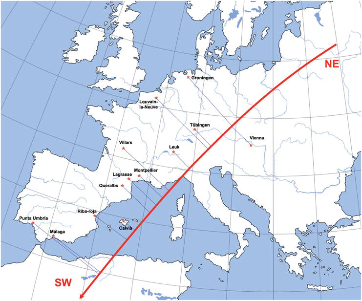
2. Obtain an interpretable direction in this Euclidean space, in terms of a geographic cline according to the results of a previous paper [11] using only European populations, see Figure 1 and Table 1.

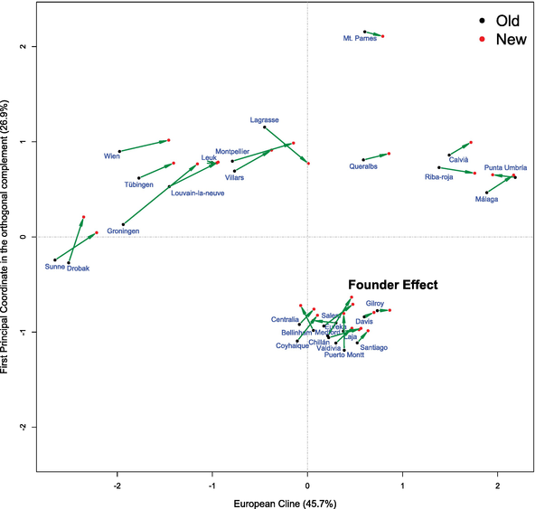
3. Once this direction has been established, we shall find another direction orthogonal to the first, with all the data, carrying out a standard PCA but onto the orthogonal complement space of the previously mentioned first direction, obtaining a 2D representation (Figure 2). The old and new data from the same geographic population have been represented by two points (one black dot and one red dot, respectively) joined by a time arrow, which visualizes the genetic profile changes.

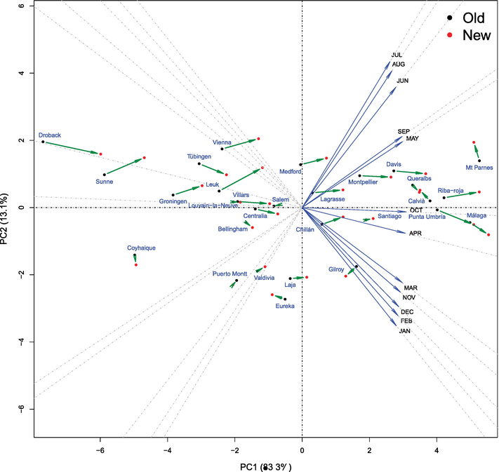
4. With the climate data, that is, mean month temperatures corresponding to the same populations and periods, we make a PCA BIPLOT analysis, interpreting the first two components as warm weather and extreme (inter-seasonal) weather, obtaining also a 2D representation (Figure 3). The old and new temperature data from the same geographic population are also represented as two points joined by a time arrow, which visualizes the mean temperature changes.

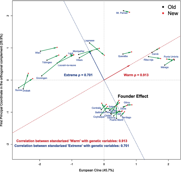
5. Finally, we integrate both types of information representing the first and second principal components of climate data analysis into the 2D genetic space representation (Figure 4).

Figure 1.

European populations and their relationship with respect to the NE to SW cline. The data can be seen in Table 1.

Population	Longitude/latitude	NE to SW in °	First component
Groningen	53°13′N–6°35′E	0.00°	−1.914748
Wien	48°13′N–16°22′E	0.03°	−1.952958
Louvain-la-neuve	50°43′N–4°37′E	3.20°	−1.429999
Tübingen	48°32′N–9°04′E	3.24°	−1.749663
Leuk	46°19′N–7°39′E	5.85°	−0.981962
Villars	45°26′N–0°44′E	9.93°	−0.743784
Montpellier	43°36′N–3°53′E	10.08°	−0.766615
Lagrasse	43°05′N–2°37′E	11.18°	−0.427634
Queralbs	42°13′N–2°10′E	12.18°	0.611528
Calvià	39°33′N–2°29′E	14.35°	1.513612
Riba-roja	39°33′N–0°34′W	15.96°	1.407313
Málaga	36°43′N–4°25′W	20.37°	1.909295
Punta Umbría	37°10′N–6°57′W	21.54°	2.208420

Table 1.

Longitude and latitude of European geographic populations. Also given are degrees with respect to the NE and SW direction. See also Figure 1. The correlation with the first principal component obtained with the 13 European geographic populations at the first time period is $r=0.9628$.

Figure 2.

2D representation of the abstract genetic space with the 29 geographic populations studied in two periods. The genetic profile changes are visualized by the arrows. The populations of the old period of time studied are represented with black dots and, in the new period of time, in red dots.

Figure 3.

2D BIPLOT with climate data. The 29 geographic populations are studied in two periods. The temperature changes are visualized by the arrows. The populations of the old period of time studied are represented with black dots, and the new period of time are in red dots. Each one of the variables, mean month standardized temperatures, is represented as blue straight lines whose direction vectors are the gradient of each variable (up to a proportionality constant: Scaled for legibility reasons) and therefore indicates its maximum increase by unit length. The horizontal axis may be interpreted as warm climate (increasing to the right) and extreme interseasonal climate (increasing upward).

Figure 4.

2D dynamic diagram genetic space and climate. Note that changes in the genetic profile are compatible with an adaptation to a warm climate.

2.1 Genetic data

We dispose of data of the chromosomal inversion frequencies corresponding to the five chromosomes of Drosophila subobscura in several European and American populations, each of them sampled in the same geographical places but at two different periods widely separated in the time, 24 years on average. Thus, although we have a total of 29 geographic populations, we shall consider a total of $N=29\times 2=58$ statistical populations (29 old and 29 new). Let $k=5$ be the number of chromosomes analyzed (A, J, U, E, and O) and $m_1,\dots ,m_k$ the number of different chromosomal arrangements located on chromosome A, J, U, E, and O, respectively. Then, given a statistical population $P_{\alpha }$, we denote by $\left(p_{\mathit{\alpha i}1},\dots ,p_{\alpha {\mathit{im}}_i}\right)$ a vector whose components are the relative frequencies of each chromosomal arrangement located on the $i$ chromosome at population $P_{\alpha }$, with $p_{\mathit{\alpha ij}}\ge 0$ where ${\sum }_{j=1}^{m_i}{p}_{\mathit{\alpha ij}}=1$ with $i=1,\dots ,k$ and $\alpha =1,\dots ,N$. Further details on the data may be found in [11, 12].

Thus, each geographic population at a given time is characterized as point $P$ in a Genetic Space, $P$, a point determined by

$$P=\left(p_{11},\dots ,p_{1m_1},p_{21},\dots ,p_{2m_2},\dots ,p_{k1},\dots ,p_{{\mathit{km}}_k}\right)$$E1

From a mathematical point of view, this space is a manifold with boundary of dimension $n={\sum }_{i=1}^k{m}_i-k$, with coordinate system defined through (1). In the present study, ${\sum }_{i=1}^k{m}_i=50$, and $n=45$.

If we consider a discrete multivariate Bernoulli distribution corresponding to each chromosome and we assume independence between them, it is well known that the Fisher information matrix induces a Riemannian structure [13] in the considered manifold that represents the genetic space whose distance will be given in terms of the square root of the sum of squares of the information metric between multivariate Bernoulli distribution corresponding to each chromosome, these being equal to the Bhattacharyya distance, up to at most a multiplicative factor, that is, the distance between two points $P_{\alpha }$ and $P_{\beta }$ of coordinates determined by $\left(p_{\alpha 11},\dots ,p_{\alpha {\mathit{km}}_k}\right)$ and $\left(p_{\beta 11},\dots ,p_{\beta {\mathit{km}}_k}\right)$, respectively, will be

$$d\left(P_{\alpha },P_{\beta }\right)=2\sqrt{\sum _{i=1}^k{\left(arccos\left(\sum _{j=1}^{m_i}\sqrt{p_{\mathit{\alpha ij}}{p}_{\mathit{\beta ij}}}\right)\right)}^2}\alpha ,\beta =1,\dots ,N$$E2

Although we do not know the exact coordinates of each statistical population, we have available reasonable estimations of them that, for the sake of simplicity, we shall denote in the same way $\left(p_{\alpha 11},\dots ,p_{\alpha {\mathit{km}}_k}\right)$ and $\left(p_{\beta 11},\dots ,p_{\beta {\mathit{km}}_k}\right)$, respectively.

Therefore, from (2), we can obtain a $N\times N$ square matrix $\mathit{D}=\left(d\left(P_{\alpha },P_{\beta }\right)\right)$, whose entries are the estimated distances between all pairs of the $N=58$ studied statistical populations. This distance, up to a multiplicative factor, was already used in [11], with a subset of the data analyzed in the present paper corresponding to 13 geographic European populations in two different time periods ($N_E=13\times 2=26$ statistical populations).

From this distance matrix, we can carry out a principal coordinate analysis (PCoA) [14, 15]. Specifically, if we let ${\mathbf{1}}_N$ be a $N\times 1$ vector whose entries are all equal to 1, ${\mathit{I}}_N$ the $N\times N$ identity matrix $\mathit{H}={\mathit{I}}_N-\frac{1}{N}{\mathbf{1}}_N{{\mathbf{1}}_N}^t$, where the symbol ${}^t$ indicates the transpose vector or matrix, the $N\times N$ centering matrix $\mathit{A}=\frac{1}{2}\mathit{D}\circ \mathit{D}$, where $\circ$ denotes the Hadamard product, we can obtain a spectral decomposition in matrix form $\mathit{A}=\mathit{Q}\mathtt{\Lambda }{\mathit{Q}}^t$ where $\mathtt{\Lambda }$ is a $N\times N$ diagonal matrix with the ordered eigenvalues of $\mathit{A}$ ${\lambda }_1\ge {\lambda }_2\ge ,\dots ,\ge {\lambda }_N$ and $\mathit{Q}$ is a $N\times N$ ortonormal matrix with the corresponding normalized eigenvectors. The eigenvalues obtained range from ${\lambda }_1=84.86376$ to ${\lambda }_N=-0.2118237$, being strictly positive the 38 first eigenvalues. Furthermore, ${\sum }_{i=1}^{38}{\lambda }_i=176.8488$_, whereas ${\sum }_{i=39}^{58}{\lambda }_i=-0.5911$. The positive part is approximately the $99.67\%$ of the addition of the absolute value of all eigenvalues. This fact suggests the possibility to map each one of the $N=58$ statistical populations into a point in ${\mathbb{R}}^q$ where $q=38$ with coordinates given by the 38 first principal coordinates. If $\tilde{\mathit{Q}}$ is the $N\times q$ matrix with the first 38 columns of $\mathit{Q}$ and $\tilde{\mathtt{\Lambda }}$ is the $q\times q$ diagonal matrix of the strictly positive ordered eigenvalues ${\lambda }_1\ge \dots ,\ge {\lambda }_q>0$, the 38 principal coordinates of the statistical populations are the rows of the $N\times q$ matrix $\mathit{X}$ given by

$$\mathit{X}=\tilde{\mathit{Q}}{\tilde{\mathtt{\Lambda }}}^{1/2}$$E3

The ordinary Euclidean distance between the rows of $\mathit{X}$ almost reproduces the original distance given in (2). In other words, if we identify each statistical population $P_{\alpha }$, with $\alpha =1,\dots ,N$ as a point that has $q=38$ Euclidean coordinates $\left(x_{\alpha 1},\dots ,x_{\mathit{\alpha q}}\right)$ such that the ordinary Euclidean distance among them,

$$d_E\left(P_{\alpha },P_{\beta }\right)=\sqrt{\sum _{i=1}^q{\left(x_{\mathit{\alpha i}}-x_{\mathit{\beta i}}\right)}^2}\alpha ,\beta =1,\dots ,N$$E4

is very similar to $d\left(P_{\alpha },P_{\beta }\right)$. Moreover, we can build the interdistance Euclidean matrix $N\times N$, ${\mathit{D}}_E=\left(d_E\left(P_{\alpha },P_{\beta }\right)\right)$, obtaining the following measures:

• Kruskal Stress [15, 16]

$$\mathit{\text{Stress}}\left(\mathit{D},{\mathit{D}}_E\right)=\sqrt{\frac{{\sum }_{i,j=1}^N{\left(d\left(P_{\alpha },P_{\beta }\right)-d_E\left(P_{\alpha },P_{\beta }\right)\right)}^2}{{\sum }_{i,j=1}^{q}d{\left(P_{\alpha },P_{\beta }\right)}^2}}=0.0030$$E5

this small Kruskal Stress indicates that $\mathit{D}$ and ${\mathit{D}}_E$ are almost equal.

• Another measure that suggests a similar behavior of both distances is the Pearson correlation between the entries of both matrices,

$$\rho \left(\mathit{D},{\mathit{D}}_E\right)=0.99999$$E6

• And the following measure, similar to a relative error of the approximation, gives

$$\mathit{Rel}.\mathit{\text{Error}}\left(\mathit{D},{\mathit{D}}_E\right)=\frac{{\sum }_{i,j=1}^N\mid d\left(P_{\alpha },P_{\beta }\right)-d_E\left(P_{\alpha },P_{\beta }\right)\mid }{{\sum }_{i,j=1}^{q}d\left(P_{\alpha },P_{\beta }\right)}=0.00248$$E7

this small relative error also indicates that $\mathit{D}$ and ${\mathit{D}}_E$ are almost equal.

All these measures indicate a great similarity between (2) and (4) and suggest using, for simplicity, the representation of the $N=58$ statistical populations in ${\mathbb{R}}^q$, with the ordinary Euclidean distance as the abstract genetic space into which we represent all of our statistical populations because their proximity relations using the Euclidean distance (4) are almost the same that the ones obtained with (2) proposed initially. The sum of squares between this distance of all considered point will be

$${\mathit{SD}}_E^2=\sum _{\alpha =1}^N\sum _{\beta =1}^N{d}_E^2\left(P_{\alpha },P_{\beta }\right)=2N\mathrm{tr}\left({\mathit{X}}^t\mathit{HX}\right)$$E8

The next step is to obtain a good two-dimensional Euclidean representation that helps us interpret the observed genetic variability. To achieve this purpose, it is important to maximize the variability explained in the 2D graphic output compared with the total variability in the whole Euclidean space ($q=38$ dimensions). This could be obtained by performing a simple PCA from the data matrix $\mathit{X}$ [8, 9, 10, 15, 16, 17, 18].

We also look for easily interpretable directions in this abstract Euclidean genetic space. Specifically, we will obtain an interpretable direction of this space that will be used as the first axis of the 2D graphic output, that is to say, we will try to interpret a direction of such space in terms of the northeast-southwest ($\mathit{NE}$-$\mathit{SW}$) geographic cline described in [11]. In that paper, this cline was identified as the first component of a principal coordinate analysis realized using (2), up to a proportionality constant, and obtained from the data corresponding with the 13 first European populations considered in the present chapter in the two time periods considered.

To obtain in our abstract genetic space the direction linked with the geographic cline described in [11], we shall find the first principal component obtained from the first $13\times 2=26$ rows of data matrix $\mathit{X}$, which correspond to the European populations studied in [11]. This component will be linked to the geographic cline because (2) and (4) are very similar. Specifically, let ${\mathit{X}}_{\epsilon }$ be the $26\times 38$ matrix with the 26 first rows of $\mathit{X}$, and ${\mathit{X}}_{\rho }$ be the $32\times 38$ matrix with the remaining rows of $\mathit{X}$, that is, ${\mathit{X}}^t=\left({\mathit{X}}_{\epsilon }^t,{\mathit{X}}_{\rho }^t\right)$. The direction searched will be given by the first principal component obtained from ${\mathit{X}}_{\epsilon }$. To obtain a PCA with these data, with the same basic notation as before, if we let ${\mathbf{1}}_{\epsilon }$ be a $r\times 1$ vector whose entries are all equal to 1, with $r=26$, ${\mathit{I}}_{\epsilon }$ the $r\times r$ identity matrix, and ${\mathit{H}}_{\epsilon }={\mathit{I}}_{\epsilon }-\frac{1}{r}{\mathbf{1}}_{\epsilon }{\mathbf{1}}_{\epsilon }^t$ where the symbol ${}^t$ indicates the transpose vector or matrix, the $r\times r$ centering matrix, we can build the covariance matrix corresponding to the abstract data matrix ${\mathit{X}}_{\epsilon }$, a $38\times 38$ matrix given by ${\mathit{S}}_{\epsilon }={\mathit{X}}_{\epsilon }^t{\mathit{H}}_{\epsilon }{\mathit{X}}_{\epsilon }/r$. Then, we will diagonalize this matrix; and because we have $r=26$ points in an Euclidean space, there will be a maximum of $25$ strictly positive covariance matrix eigenvalues, ${\lambda }_{\epsilon 1}\ge {\lambda }_{\epsilon 2}\ge \dots \ge {\lambda }_{\mathit{\epsilon p}}>0$, obtaining a spectral decomposition whose matrix form may be expressed as ${\mathit{S}}_{\epsilon }={\mathit{U}}_{\epsilon }{\mathit{D}}_{\epsilon }{\mathit{U}}_{\epsilon }^t$, where ${\mathit{D}}_{\epsilon }$ is a diagonal $p\times p$ matrix with the obtained ordered positive eigenvalues, and ${\mathit{U}}_{\epsilon }$ is a $q\times p$ matrix whose columns are normalized eigenvector corresponding to the aforementioned positive eigenvalues. The first principal component, given by the first column of ${\mathit{U}}_{\epsilon }$, referred hereafter simply as the $38\times 1$ column vector $\mathit{u}$, it will be the direction in the abstract $q$-dimensional genetic space linked with the geographic cline. This direction summarizes the $100{\lambda }_{\epsilon 1}/\mathrm{tr}\left({\mathit{S}}_{\epsilon }\right)=69.3\%$ variability of the statistical populations corresponding to European populations. The correlation between the first component obtained and the first principal coordinate analysis described in [11] corresponding to the old data is $-0.999999$, which indicates the same direction. The negative sign is simply due to the fact that we choose the sign of the first component obtained to be positively correlated with the geographic cline oriented from the $\mathit{NE}$ to $\mathit{SW}$, see Table 1.

To clearly show the relationship between the first component and the northeast to southwest geographic cline, we can correlate a measurement in degrees along the $\mathit{NE}$ to $\mathit{SW}$ cline, say $\mathit{NE}/\mathit{SW}$, from 0.00° of Groningen to 21.54° of Punta Umbría, obtained through the standard latitude and longitude coordinates of the different populations, with the values of the first principal component of each geographic population at the old time period studied, say ${\mathit{Y}}_{\mathit{\text{εold}}}$, obtaining a correlation $\rho \left(\mathit{NE}/\mathit{SW},{\mathit{Y}}_{\mathit{\text{εold}}}\right)=0.9628$, see Table 1.

Next, to obtain the second direction of the abstract genetic space that we will use to obtain the 2D representation, we will project all 58 points that represent each statistical population onto the orthogonal complement space of the span of $\mathbf{u}$, ${⟨\mathbf{u}⟩}^{\perp }$. On this 37-dimensional space, we will carry out a standard PCA and will use the first principal component, say the $q\times 1$ column vector $\mathbf{v}$, orthogonal to $\mathbf{u}$ and unitary, on the projected points on ${⟨\mathbf{u}⟩}^{\perp }$ as the second direction of the space where we will project all the points, namely, the span of $\mathbf{u}$ and $\mathbf{v}$, $⟨\mathbf{u},\mathbf{v}⟩$. Specifically, the projection onto ${⟨\mathbf{u}⟩}^{\perp }$ is realized by means of the product $\mathbf{X}\left(\mathbf{I}-{\mathbf{uu}}^t\right)$, where $\mathbf{I}$ is the $38\times 38$ identity matrix; this $N\times q$ matrix with the coordinates of the $N=58$ populations in ${⟨\mathbf{u}⟩}^{\perp }$ is a centered matrix, and its covariance will be $\mathbf{S}=\left(\mathbf{I}-{\mathbf{uu}}^t\right){\mathbf{X}}^t\mathbf{X}\left(\mathbf{I}-{\mathbf{uu}}^t\right)/N$.

Then, we will diagonalize this matrix $\mathbf{S}$ and will have a maximum of $q=38$ strictly positive covariance matrix eigenvalues, ${\lambda }_1\ge {\lambda }_2\ge \dots \ge {\lambda }_q\ge 0$, obtaining a spectral decomposition whose matrix form can be expressed as $\mathbf{S}=\mathbf{V}\mathtt{\Lambda }{\mathbf{V}}^t$, where $\mathtt{\Lambda }$ is a diagonal $q\times q$ matrix with the obtained ordered positive eigenvalues, and $\mathbf{V}$ is a $q\times q$ matrix whose columns are normalized orthogonal eigenvector corresponding to the aforementioned eigenvalues. The first principal component will be given by the first column of $\mathbf{V}$, referred hereafter simply as the $q\times 1$ column vector $\mathbf{v}$; it will define the direction in the abstract $q$-dimensional genetic space that we shall use to complete the desired 2D representation. The direction determined by $\mathbf{v}$ summarizes the $100{\lambda }_1/\mathrm{tr}\left(\mathbf{S}\right)=49.2\%$ variability of the statistical populations corresponding to all populations in ${⟨\mathbf{u}⟩}^{\perp }$. The 2D final plot will be obtained with the projection of the rows of $\mathbf{X}$ into the span of $\mathbf{u},\mathbf{v}$, namely, $⟨\mathbf{u},\mathbf{v}⟩$. Introducing the $q\times 2$ matrix $\mathbf{P}=\left(\mathbf{u},\mathbf{v}\right)$, that is, a two column matrix whose columns are the column vectors $\mathbf{u}$ and $\mathbf{v}$, the coordinates of the $N$ statistical populations will be rows of the $N\times 2$ matrix $\mathbf{Y}=\left(y_{\mathit{\alpha j}}\right)$ given by

$$\mathbf{Y}=\mathbf{XP}$$E9

We can easily quantify the percentage of variability represented by each one of the 2D-plot axes, computing first the sum of the squared distance between all the points if we project them in the first axis, ${\mathit{SD}}_{a1}^2$ and in the second one ${\mathit{SD}}_{a2}^2$ of the plot, that is

$${\mathit{SD}}_{\mathit{ai}}^2=\sum _{\alpha =1}^N\sum _{\beta =1}^N{\left(y_{\mathit{\alpha i}}-y_{\mathit{\beta i}}\right)}^2\text{with}i=1,2$$E10

and comparing these quantities with the total variability ${\mathit{SD}}_E^2$ given in (8), we obtain the percentages ${\theta }_{\mathit{ai}}$ given by ${\theta }_{\mathit{ai}}=100\times {\mathit{SD}}_{\mathit{ai}}^2/{\mathit{SD}}_E^2$ with $i=1,2$, which in the present case are equal to ${\theta }_{a1}=45.5\%$ and ${\theta }_{a2}=26.8\%$, thus, the variability explained by both axis ${\theta }_{a1}+{\theta }_{a2}$ will be equal to $72.3\%$. We can see the described 2D representation in Figure 2; the coordinates of the populations are given by the Eq. (9).

To interpret the change of the genetic profile of the 29 geographic populations between the two periods studied, separated in time on average in just over 24 years, it will be convenient to define two $29\times 1$ column vectors ${\mathbf{Y}}_1$ and ${\mathbf{Y}}_2$ that contains the two coordinates of each one of the 29 populations in the plot, the populations located in the same order in both vectors, at the old period ${\mathbf{Y}}_1$ and at the new one ${\mathbf{Y}}_2$. The change of the genetic profiles of each geographic population between periods may be visualized by $\mathit{\delta }={\mathbf{Y}}_2-{\mathbf{Y}}_1$, given by the green arrows in Figure 3 from the black points (populations of the old time period) to the red points (populations of the new time period) (Table 2).

Population	${\mathit{\delta }}_1$	${\mathit{\delta }}_2$	Population	${\mathit{\delta }}_1$	${\mathit{\delta }}_2$
Montpellier	0.642373	0.190589	Lagrasse	0.459498	−0.381803
Queralbs	0.268763	0.066369	Riba-roja	0.374971	−0.059232
Calvià	0.228700	0.134521	Punta Umbría	−0.237194	0.027191
Málaga	0.282278	0.184082	Groningen	0.780543	0.635947
Louvain-la-neuve	0.513534	0.256845	Villars	0.389008	0.219267
Tübingen	0.364991	0.157145	Wien	0.516528	0.118356
Leuk	0.050395	−0.004103	Sunne	0.438114	0.288466
Drobak	0.158006	0.481837	Mt. Parnes	0.189012	−0.047603
Gilroy	0.130422	0.004212	Davis	0.101785	0.046262
Eureka	0.305773	0.228315	Medford	0.251930	0.405888
Salem	−0.241229	0.023833	Centralia	0.153696	0.160464
Bellinham	−0.133972	0.262271	Santiago	0.113615	0.127641
Chillán	0.339739	0.097727	Laja	0.164784	0.015877
Valdivia	0.168553	0.155098	Puerto Montt	−0.005071	0.386463
Coyhaique	0.212375	0.270840	–	–	–

Table 2.

The components of vectors $\mathit{\delta }=\left({\mathit{\delta }}_1,{\mathit{\delta }}_2\right)$ represent the profile genetic changes in each of the 29 studied geographic populations. Observe that the 29 components of ${\mathit{\delta }}_1$, the first column vector of $\mathit{\delta }$, are positive in 25 of the 29 cases (each one corresponding to a different population). The shift is compatible with profiles more adapted to the climate of $\mathbf{SW}$.

The few negative values in the second column are highlighted in contrast to the majority of the positive values.

Additionally, among the total of 29 geographic populations considered, in 25 of them in the course of the time between the first and the second period of time studied, a displacement occurs, increasing the value of the first variable used for the 2D representation, which is a direction that represents the $\mathbf{NE}/\mathbf{SW}$ cline. Moreover, this low value is hardly compatible with a random change (in an ordinary bilateral sign test, $p-\text{value}\approxeq 1.0\times {10}^{-4}$). Let us also observe the limited dispersion of American populations, as a consequence of the so-called founder effect produced by the recent colonization of Drosophila subobscura to the New World in the late 70s of the last century when this species was accidentally introduced to America. This effect refers to the reduction of genomic variability due to a small group of individuals separating from the original population [12].

2.2 Climate data

Along with the data analysis of chromosomal polymorphisms in Drosophila subobscura, we recorded meteorological data for the 4 years immediately preceding each biological sample from the nearest meteorological station for each population using NASA GISS. (http://data.giss.nasa.gov/gistemp/) and NOAA (http://www.ncdc.noaa.gov/oa/climate/climatedata.html). Then, we calculate the average monthly temperatures during these 4 years, in degrees Celsius, seasonally adjusting them and taking into account the hemisphere of origin. Thus, to each of the statistical populations considered $\left(N=58=29\times 2\right)$, we will associate a vector in ${\mathbb{R}}^{12}$ whose components are precisely the average temperature values per month, using standardized data to make the analysis invariant under linear changes. Then, we perform an ordinary PCA. Specifically, let $\mathbf{W}=\left(w_{\mathit{\alpha j}}\right)$ be a $58\times 12$ real matrix whose entries are the month mean values attached to each statistical population determined by the 29 different geographic sites and two periods, from January to December, seasonally adjusted by hemisphere (for instance, January is the real January in the northern hemisphere but July in the southern hemisphere and similar with the other months) and already standardized. Then, with the same basic notation as before, we can compute the corresponding covariance matrix equal to the correlation matrix because the data are standardized, given by ${\mathbf{R}}_{\mathbf{W}}={\mathbf{W}}^t\mathbf{HW}/N$. Then, we will diagonalize this matrix and obtain 12 ordered nonnegative eigenvalues ${\lambda }_1\ge {\lambda }_2\ge \dots \ge {\lambda }_{12}\ge 0$ obtaining a spectral decomposition whose matrix form may be expressed as ${\mathbf{R}}_{\mathbf{W}}=\mathbf{T}\mathtt{\Gamma }{\mathbf{T}}^t$, where $\mathtt{\Gamma }$ is a diagonal $12\times 12$ matrix with the ordered nonnegative eigenvalues, and $\mathbf{T}$ is a $12\times 12$ orthogonal matrix whose columns are normalized eigenvector corresponding to the aforementioned nonnegative eigenvalues. Because ${\lambda }_1=10.00127$, the first principal component given by the first column of $\mathbf{T}$ summarizes the $83.3\%$ of mean temperature variance; whereas since ${\lambda }_2=1.56655$, the second principal component, given by the second column of $\mathbf{T}$ summarizes the $13.1\%$ of mean temperature variance. Therefore, the two main principal components summarizes the $96.4\%$ of mean temperature total variance. Explicitly, introducing the $12\times 2$ matrix $\mathtt{\Upsilon }=\left({\mathbf{t}}_1,{\mathbf{t}}_2\right)$, where ${\mathbf{t}}_1$ and ${\mathbf{t}}_2$ are the first two columns of $\mathbf{T}$ and these two components on the $N=58$ statistical populations will be given by the two columns of the $N\times 2$ matrix $\mathbf{C}=\left({\mathbf{c}}_1,{\mathbf{c}}_2\right)=\left(c_{\mathit{\alpha j}}\right)$ with $j=1,2$ given by

$$\mathbf{C}=\mathbf{W}\mathtt{\Upsilon }$$E11

Classical PCA BIPLOT of climate data, see Figure 3, where the populations (labeled in blue) and climate variables (arrows in blue) are represented. The coordinates of the populations corresponding to the old temperature measurements appear in black and the coordinates corresponding to the new measurements (taken 4 years later as average) appear in red. It will be convenient to interpret the variables in order to compute the loadings of the principal components to each variable, and these quantities also obtain a standard BIPLOT [19, 20].

The different variables (from January to December) can be represented by different straight lines through the origin. Table 3 can facilitate the interpretation of the principal components. Because the coefficients determining the first principal component are all positive, we can interpret this component as a size-related component. Specifically, associated with higher temperature, let us call warm climate the first component direction. The blue arrows show the displacement of the populations induced by the time interval. We observe that the arrows are mostly aligned with the first component and, consequently, aligned with an increase of mean temperatures: a shift to a Warmer climate. We can interpret the second principal component as a component related to interseasonal extreme weather, since the loadings of the warmer month are positives and negative the loadings of colder months let us call extreme climate the second component direction.

Population/month	January	February	March	April	May	June
Droback old	−7.025	−8.850	−4.050	2.150	7.975	12.800
Málaga new	14.075	14.825	16.075	17.275	19.250	22.000
Vienna new	0.375	1.725	5.550	10.700	16.350	20.025
Eureka old	9.533	8.833	9.867	10.233	12.175	13.625
Population/month	July	August	September	October	November	December
Droback old	16.600	13.950	9.900	4.725	−1.200	−5.175
Málaga new	24.000	24.575	22.175	20.450	17.425	15.300
Vienna new	21.025	21.525	14.825	10.375	6.125	0.100
Eureka old	14.650	15.125	14.175	12.375	10.350	9.625

Table 3.

The mean temperatures in Celsius degrees of four statistical populations in the different month referred to as northern hemisphere seasons, that is, we shift the data corresponding to populations of the southern hemisphere since in that hemisphere the summer period is the winter in the northern hemisphere, among others.

2.3 Climate data into the 2D genetic space representation

We can represent the first and second principal component of the previously mentioned climate data PCA into the 2D graphic obtained using only genetic data.

One way to proceed is to find the linear combination of the genetic variables (${\mathbf{Y}}_1$,${\mathbf{Y}}_2$) that have the maximum correlation with the first and second principal components of climate data ${\mathbf{c}}_1$ and ${\mathbf{c}}_2$, that is, find the coefficients ${\mathit{\alpha }}^t=\left({\alpha }_1,{\alpha }_2\right)$ and ${\mathit{\beta }}^t=\left({\beta }_1,{\beta }_2\right)$ such that

$$\underset{{\mathit{\alpha }}^t=\left({\alpha }_1,{\alpha }_2\right)}{argmax}\mathit{cor}\left({\mathbf{c}}_1,{\alpha }_1{\mathbf{y}}_1+{\alpha }_2{\mathbf{y}}_2\right)\underset{{\mathit{\beta }}^t=\left({\beta }_1,{\beta }_2\right)}{argmax}\mathit{cor}\left({\mathbf{c}}_2,{\beta }_1{\mathbf{y}}_1+{\beta }_2{\mathbf{y}}_2\right)$$E12

The direction defined by ${\mathit{\alpha }}^t=\left({\alpha }_1,{\alpha }_2\right)$ is the linear combination of the abstract genetic variables ${\mathbf{Y}}_1$ and ${\mathbf{Y}}_2$ that fit the most with the first temperature component ${\mathbf{c}}_1$. In a similar way, the direction defined by ${\mathit{\beta }}^t=\left({\beta }_1,{\beta }_2\right)$ is the linear combination of the abstract genetic variables ${\mathbf{Y}}_1$ and ${\mathbf{Y}}_2$ that best fits with the second temperature component ${\mathbf{c}}_2$.

After some straightforward computation, the sought coefficients $\mathit{\alpha }$ and $\mathit{\beta }$ that define the previously mentioned directions in the abstract genetic space and that imply unit variance of the vectors $\mathbf{Y}\mathit{\alpha }$ and $\mathbf{Y}\mathit{\beta }$ are given by

$$\mathit{\alpha }=\frac{{\left({\mathbf{Y}}^t\mathbf{Y}\right)}^{-1}{\mathbf{Y}}^t{\mathbf{c}}_1}{\sqrt{{\mathbf{c}}_1^t\mathbf{Y}{\left({\mathbf{Y}}^t\mathbf{Y}\right)}^{-1}{\mathbf{Y}}^t{\mathbf{c}}_1}}\text{and}\mathit{\beta }=\frac{{\left({\mathbf{Y}}^t\mathbf{Y}\right)}^{-1}{\mathbf{Y}}^t{\mathbf{c}}_2}{\sqrt{{\mathbf{c}}_2^t\mathbf{Y}{\left({\mathbf{Y}}^t\mathbf{Y}\right)}^{-1}{\mathbf{Y}}^t{\mathbf{c}}_2}}$$E13

and the achieved maximum correlation with ${\mathbf{c}}_1$ and ${\mathbf{c}}_2$ are respectively

$${\rho }_1=\frac{\sqrt{{{\mathbf{c}}_1}^t\mathbf{Y}{\left({\mathbf{Y}}^t\mathbf{Y}\right)}^{-1}{\mathbf{Y}}^t{\mathbf{c}}_1}}{\sqrt{{{\mathbf{c}}_1}^t{\mathbf{c}}_{\mathbf{1}}}}\text{and}{\rho }_2=\frac{\sqrt{{{\mathbf{c}}_2}^t\mathbf{Y}{\left({\mathbf{Y}}^t\mathbf{Y}\right)}^{-1}{\mathbf{Y}}^t{\mathbf{c}}_2}}{\sqrt{{{\mathbf{c}}_2}^t{\mathbf{c}}_{\mathbf{2}}}}$$E14

In the present example, we obtain ${\rho }_1=0.913466$ that shows that the direction corresponding to the first component of the PCA in Figure 4 are closely linearly related with warm climate, whereas the value obtained for ${\rho }_2=0.700762$ shows an important although weaker linear relationship of the direction corresponding to the second principal component in Figure 4, interpreted as extreme climate.

Furthermore, to study the relationship of the variable which represents the Warm climate with the observed shifts of the genetic population profiles of each geographic population at different times, given by $\mathit{\delta }$, the green arrows from the black points (populations of the old time period) to the red points (populations of the new time period), we can compute the scalar product of these vectors $\mathit{\delta }$ with the variable $\mathbf{Y}\mathit{\alpha }$. Among the total of 29 geographic populations considered, in 27 (all with the exception of Punta Umbría and Salem) of them this scalar product is positive indicating that the shift is compatible with a genetic adaptation to a warmer climate. Moreover, this low value is hardly compatible with a random change (in an ordinary bilateral sign test, $p-\text{value}\approxeq 1.6\times {10}^{-6}$) (Table 4).

Population	$⟨{\mathit{\delta }}_i,\mathrm{Y}\mathit{\alpha }⟩$	$⟨{\mathit{\delta }}_i,\mathrm{Y}\mathit{\beta }⟩$	Population	$⟨{\mathit{\delta }}_i,\mathrm{Y}\mathit{\alpha }⟩$	$⟨{\mathit{\delta }}_i,\mathrm{Y}\mathit{\beta }⟩$
Montpellier	0.601249	−0.121418	Lagrasse	0.191069	−0.548328
Queralbs	0.245389	−0.062709	Riba-roja	0.272323	−0.222716
Calvià	0.244812	0.016150	Punta Umbría	−0.177003	0.131730
Málaga	0.310490	0.036006	Groningen	0.917106	0.212613
Louvain-la-neuve	0.528855	−0.004008	Villars	0.412010	0.018966
Tübingen	0.364161	−0.025477	Wien	0.467364	−0.128710
Leuk	0.038379	−0.026496	Sunne	0.483173	0.058340
Drobak	0.348535	0.357530	Mt. Parnes	0.129084	−0.128070
Gilroy	0.106166	−0.055364	Davis	0.102679	−0.004933
Eureka	0.349669	0.064752	Medford	0.388557	0.247314
Salem	−0.181777	0.130567	Centralia	0.196843	0.073252
Bellinham	0.013925	0.294317	Santiago	0.149672	0.062186
Chillán	0.316573	−0.066951	Laja	0.139006	−0.060550
Valdivia	0.206240	0.061739	Puerto Montt	0.174221	0.346502
Coyhaique	0.294650	0.144961	–	–	–

Table 4.

The second and fifth columns show the scalar product between ${\mathit{\delta }}_i$ and $\mathbf{Y}\mathit{\alpha }$. Analogously, the third and sixth columns provide the scalar product between ${\mathit{\delta }}_i$ and $\mathbf{Y}\mathit{\beta }$, where $\mathbf{Y}\mathit{\alpha }$ is the direction that represents warm climate in the 2D representation of the genetic spaces and $\mathbf{Y}\mathit{\beta }$ is the direction which represents extreme climate in the 2D representation of the genetic space. Observe that the scalar product between ${\mathit{\delta }}_i$ and $\mathbf{Y}\mathit{\alpha }$ is positive in almost all population, which is compatible with a profile shift to more warm adapted genetic configurations.

The few negative values in the second column are highlighted in contrast to the majority of the positive values.

3. Conclusions

In this work, we illustrate a procedure that combines dimension reduction for temporal data and the integration of multiple multivariate sources, in our case, genetic data and climate data. We have proposed a formulation to enrich dimension reduction by choosing interpretable directions in the representation space rather than maximizing variability.

Analysis of the genetic data consistently reveals a shift of populations along the European northeast to southwest cline when comparing the two time periods. On the other hand, the analysis of climate data reveals a first component associated with warm climate. At the same time, a shift of populations in the direction of higher temperature is observed when comparing time points. When we integrate the climatic with the genetic information, we have verified that both displacements, corresponding to the populations in the genetic space and the populations in the climate space, respectively, are highly aligned, suggesting that all populations along the cline are evolving toward the adaptation to a warm climate.

We emphasize that the methodology used in this study is very versatile and easily applicable for multivariate data integration in other areas of application.

Acknowledgments

This research was funded by the Ministerio de Ciencia e Innovación (Spain) (Ref: PID2019-104830RB-I00/AEI DOI: 10.13039/501100011033).

Conflict of interest

The authors declare no conflict of interest.

Nomenclature

PCA	principal component analysis
PCoA	principal coordinate analysis
2D ...	2 dimensional ...
NE	Northeast
SW	Southwest
NASA	National Aeronautics and Space Administration
GISS	Goddard Institute for Space Studies
NOAA	National Oceanic and Atmospheric Administration