Improvement of the Global Positioning Accuracy with Miniaturized Strap-Down INS Systems through Wavelet Filtering of Data from MEMS Inertial Sensors

Abstract

In this chapter, the correlation between the issue of perturbed data acquired from miniaturized inertial sensors and the wavelet filtering technique is investigated. The market growth of micro-electro-mechanical systems (MEMS) has impacted various fields, and its potential application in strap-down inertial navigation systems (INS) could not be overlooked. Despite the apparent benefits of dimension and price reduction, the utilization of miniaturized inertial sensors for manufacturing the inertial measurement unit (IMU) entails certain drawbacks: the output signals are usually corrupted with different types of errors, which distort the real navigation information. The proposed case focuses on the suitability of wavelets for denoising the perturbed IMU signals before being erroneously processed by the navigation algorithm. The applicative part consisted in implementing sensor software models in Simulink and testing various wavelet filters. Furthermore, to fully assess the efficacy of the wavelet denoising technique, the model of a SDINS employing a MEMS-based IMU was established in Simulink. The evaluation involved comparing the attitude, position and speed components obtained before and after the denoising procedure with those of an ideal model linked to constant inputs. The results demonstrated the effectiveness of the proposed association in terms of positioning accuracy, signal characteristics improvement and computation complexity.

1. Introduction

Micro-electro-mechanical systems gained immensely in popularity within sensor manufacturing technologies, primarily owing to their distinctive properties arising from the integration of both mechanical and electrical devices on a single chip. In the same vein, the strap-down architecture of inertial navigation systems has diminished the mechanical complexity of previous platform versions, consequently driving the demand for smaller inertial sensors [1]. The adoption of MEMS technology for the IMU fabrication of strap-down inertial navigation systems is primarily generated by the significant advantages it offers, including reduced size, cost-effectiveness, scalability in serial production, and low power consumption. However, the miniaturization process of electronic devices leads to enhanced sensitivity to external environmental factors such as temperature, humidity, and vibrations. Consequently, this increased sensitivity leads to the propagation of errors and noises in the output acceleration and angular rate signals [2]. Instead of a continuous and clear evolution representation of the measured dataset, the useful signal is often submerged in the noise. Conventional filtering methods usually prove to be inefficient and may even cause signal distortion due to the tendency of noise frequency bands to overlap with the frequency band in which the dynamics of the monitored vehicle are located [3].

In the past decade, the field of signal processing has directed its attention towards the relatively modern discovery of wavelet theory. The wavelet transform, based on multiresolution analysis, decomposes a signal into wavelet components at various scales, enabling the representation of different levels of details within the signal. Numerous applications have been found for wavelets in fields such as image processing, denoising, feature extraction, and compression, enabling efficient analysis of oscillatory phenomena in various data types [4]. Because of their ability to effectively denoise signals while preserving critical information, wavelets present a promising option to address the rigorous requirements of inertial navigation. Hence, the investigation of wavelet filters’ behavior regarding perturbed inertial data is a worthwhile subject for research.

The main objective of the experimental part was to evaluate the effectiveness of pre-filtrating the outputs of inertial sensors before incorporating them as inputs into the strap-down navigation algorithm, with a focus on the essential improvement in positioning accuracy. To set the context for the practical part, this study first provides a comprehensive overview of the types of errors associated with MEMS inertial sensors. Subsequently, a mathematical foundation is established to support the application of the wavelet denoising technique.

The experimental part presents how two MEMS sensor models—an accelerometer and a gyroscope—were software implemented and simulated with constant inputs using MATLAB/Simulink. The resulting perturbed output signals underwent decomposition using various wavelet functions, and their performances were assessed through the calculation of specific estimator measures. In the second part, the strap-down navigation algorithm was fully developed in the Simulink software environment and tested in association with the wavelet filter. The outcomes of the simulations furnished a comprehensive insight into the implications of MEMS architecture on the output data precision of the strap-down algorithm. Moreover, the extent to which wavelet techniques succeed in enhancing the overall accuracy was also rigorously assessed.

As important limitations of the proposed work can be mentioned the partial removal of the noise perturbing the inertial sensors and the offline tuning of the wavelet transform, which means that the noise coming from various sources operating near the sensors during flight cannot be limited through a real-time tuning of the involved wavelet mechanisms.

2. Preliminary analysis of the miniaturization issues

As MEMS-based sensors are scaled down to smaller dimensions, they become inherently more sensitive to external environmental factors, which can lead to adverse effects on their performance. One of the primary concerns arising from miniaturization is the increased susceptibility to external noise sources. Due to their reduced size, MEMS inertial sensors exhibit higher sensitivity to temperature fluctuations, humidity variations, and mechanical vibrations. These environmental influences can introduce unwanted perturbations and inaccuracies in the sensor’s output signals, compromising the overall measurement accuracy. Moreover, as the size of MEMS inertial sensors decreases, there is a consequent reduction in their mass and inertial properties. This reduction may lead to diminished signal-to-noise ratios, making it challenging to distinguish the desired signal from noise effectively. Consequently, the signal of interest may become masked by the noise, hindering the accurate extraction of relevant information [5].

In general, errors in MEMS inertial sensors can be categorized into two main groups: deterministic errors and stochastic errors. Deterministic errors are systematic and predictable errors that result from inherent characteristics of the sensor or external influences. They include bias error, scale factor error, misalignment error, and cross-coupling error. Stochastic errors, on the other hand, are random and unpredictable variations in the sensor’s output caused by environmental factors and noise sources. Some examples of stochastic errors are random noise, drift, vibration noise, and quantization noise [6].

Understanding and characterizing these errors is crucial for accurate sensor calibration and data interpretation. Their integration with the original signal introduces inaccuracies and uncertainties in the measured data, directly impacting the overall performance of the strap-down navigation system and potentially compromising the success of its mission. Figure 1 visually illustrates the errors that overlap a MEMS gyro’s original signal, resulting in a corrupted output. This graphical representation emphasizes the importance of utilizing denoising techniques, such as wavelet filtering, which will be widely discussed during the next section.

Figure 1.

Corrupted output signal of a MEMS gyro.

3. Wavelet denoising method

3.1 Mathematical background of wavelets

A wavelet is a mathematical function characterized by its oscillating pattern, where the amplitude initiates from zero, undergoes multiple cycles of increase and decrease, and eventually returns to zero. It allows signals to be analyzed and transformed into different frequency components, providing a way to capture both high and low-frequency oscillations in a signal.

Wavelets are particularly advantageous when dealing with signals that exhibit non-stationary or localized oscillatory behavior [4]. Figure 2 presents a visual representation of the most common types of wavelet functions.

Figure 2.

Examples of wavelet functions.

The wavelet transform is a powerful mathematical tool used in signal processing to decompose a signal into its frequency components. There are two types of wavelet transforms: continuous wavelet transform (CWT) and discrete wavelet transform (DWT). The CWT allows for continuous variation in the scale of the wavelet function, providing a detailed representation of the signal’s frequency content at different time points. On the other hand, the DWT breaks down the signal into discrete scales, which is computationally more efficient and suitable for practical applications [7].

For denoising the output signals of our miniaturized inertial sensors, the DWT is particularly well-suited. The DWT can effectively capture localized and non-stationary oscillations, making it advantageous for processing signals affected by external environmental factors and noise. By decomposing the signal into various scales, the DWT allows for a more precise analysis and separation of noise from the useful signal, resulting in improved denoising performance [8].

In the field of signal processing, various transforms, such as the Fourier Transform (FT) and the Fast Fourier Transform (FFT), have been widely employed for frequency domain analysis. While these transforms are effective in revealing the frequency content of a signal, they possess certain limitations when dealing with signals containing localized or non-stationary features [9]. Unlike the DWT, which decomposes signals into different frequency components with varying time resolutions, the FT and FFT provide a fixed frequency resolution across the entire signal, as can be observed in Figure 3.

Figure 3.

Varieties of time-frequency analysis techniques.

This characteristic restricts their ability to effectively capture localized features and may lead to signal distortion when dealing with non-stationary signals. The DWT’s adaptability to a wide range of signal characteristics, along with its ability to efficiently handle real-world data, makes it a superior choice for various signal processing tasks, including denoising, feature extraction, and pattern recognition in practical applications.

3.2 Systematic implementation of wavelet filtering

The process of filtering a perturbed signal with a wavelet function begins with selecting a suitable type of function. The choice should be made considering the specific characteristics of the noise and signal, as well as the desired denoising outcome; however, it is advisable to test multiple wavelets as they may exhibit distinct behaviors depending on the specific case.

When the chosen discrete wavelet transform (DWT) is applied to the signal, it operates as a sequence of high-pass and low-pass filters, leading to the decomposition of the signal into several sub-bands, each representing distinct frequency ranges. This procedure yields wavelet coefficients, categorized as either approximation (cA) responsible for capturing low-frequency information or details (cD) responsible for capturing high-frequency information (Figure 4) [9].

Figure 4.

DWT signal decomposition.

The process of decomposition can be iteratively performed by applying the discrete wavelet transform (DWT) to the obtained approximation coefficients (cA) from the initial decomposition stage. This recursive application results in a multi-level wavelet decomposition, as illustrated in Figure 5. Each level of the decomposition provides a new set of approximation coefficients, capturing lower frequency components successively. This hierarchical approach facilitates the analysis of the signal at various scales and resolutions, offering a comprehensive insight into its frequency content.

Figure 5.

Iterative process of wavelet decomposition.

During this stage, the concept of thresholding becomes crucial. Once the decomposition process is complete, a specific threshold is established, and each absolute value of the wavelet coefficient is subjected to comparison with this threshold. The threshold value can be computed using the following formula [10]:

$$\lambda =\sqrt{2\mathit{\text{logn}}}\sigma$$E1

where: n – number of samples, σ – standard deviation of the signal.

In wavelet denoising, two common thresholding techniques are used: soft thresholding and hard thresholding. Soft thresholding shrinks wavelet coefficients below the threshold to zero, while hard thresholding sets coefficients below the threshold to zero. The choice between the two depends on the signal characteristics and denoising goals. In the current case, soft thresholding is preferred as it offers a more gradual suppression of noise compared to hard thresholding. The perturbed navigation signals often contain various levels of noise, and the abrupt removal of coefficients through hard thresholding may cause a significant loss of useful signal information. This choice was influenced by previous successful implementations, notably in Refs. [11, 12], which also employed soft thresholding. Eq. (2) shows the soft thresholding function [10]:

$$T_{\lambda }^{\mathit{\text{soft}}}=\left\{\begin{array}{c}\left(u-\mathit{sign}\left(u\right)\right)\mathit{\lambda if}\left|u\right|\ge \lambda \\ 0\mathit{\text{othrewise}}\end{array}\right.$$E2

After the thresholding phase in the wavelet filtering procedure, the signal is restored from the adjusted wavelet coefficients. By performing the inverse wavelet transform to these coefficients, the original signal is reconstructed with reduced noise and preserved essential characteristics. This updated signal offers an improved representation of the underlying useful information, making it suitable for further analysis and applications, such as navigation and control systems.

The wavelet denoising process outlined above applied to our research case can be summarized into five key stages, as illustrated by Figure 6.

Figure 6.

Wavelet denoising method.

3.3 Filter performance evaluation criteria

In the denoising process, a crucial concern arises regarding the suitability of the chosen wavelet function and the optimal level of decomposition to repeat the procedure. To address this, several evaluation metrics can be employed, offering relevant insights into the filter’s performance in signal reconstruction. Throughout this research paper, the selected evaluation criteria include the mean square error (MSE) and signal-to-noise ratio (SNR), calculated with formulas (3) and (4) [13]:

$$\mathit{MSE}=\frac{1}{n}\sum _{i=1}^n{\left[x\left(i\right)-\stackrel{\sim }{x}\left(i\right)\right]}^2,$$E3

$$\mathit{SNR}=10{·\mathit{log}}_{10}\left\{\frac{{\sum }_{i=1}^n\left(x\left(i\right)\right)}{{\sum }_{i=1}^n{\left[x\left(i\right)-\stackrel{\sim }{x}\left(i\right)\right]}^2}\right\},$$E4

where: n – number of samples, $x\left(i\right)$ – ideal, unfiltered signal, $\stackrel{\sim }{x}\left(i\right)$– filtered signal.

Reference [11] involved comparing SNR values obtained from different wavelet functions applied to noisy acceleration signals, facilitating the ranking of their performance. Also, the addition of the last point deviation from the reference distance confirmed the previous results. In our scenario, the MSE and SNR parameters assist us in identifying the optimal decomposition level by selecting values that adhere to specified limits, while also enabling a performance comparison between the two wavelet functions (Figure 7).

Figure 7.

MATLAB/Simulink accelerometer model.

The wavelet filter’s performance, in terms of positioning accuracy improvement, can be assessed by directly analyzing the navigation information before and after the denoising procedure. This evaluation included a comparison with an ideal model of the strap-down navigation algorithm that utilizes unperturbed inputs. The ideal model gave conceptual values representing the expected outputs if the sensor data were not affected by perturbations. By contrasting the denoised navigation information with these conceptual values, the effectiveness of the wavelet filter in enhancing positioning accuracy can be determined.

4. Software configuration of the MEMS-based IMU and wavelet filter association

4.1 Inertial sensors software implementation

An IMU is the main sensing component of any INS and it is generally composed of two triads of inertial sensors—accelerometers for sensing the specific force and gyros for the angular rate, both being rigidly attached to the body of the vehicle. In order to achieve precise and realistic results in a comprehensive study that mirrors the actual conditions of the navigation system, including the inherent errors of the sensors employed, it becomes imperative to establish an equivalent model. To create the software representation of an IMU, the process was initiated by implementing an accelerometer and a gyro in MATLAB/Simulink using IEEE standardized models [3, 14].

The accelerometer model follows the equation:

$$a=\left(a_i+N·a_i+B+k_c{a}_c+\nu \right)\left(1+\frac{\mathit{\Delta K}}{K}\right),$$E5

where: a – output acceleration (perturbed signal), N – misalignment of the sensitive axis, a_i – acceleration applied along the sensitive axis, B – bias, k_c – cross-axis sensitivity, a_c – cross-axis acceleration, B – bias, ν – noise, K – scale factor, ΔK – calibration error of the scale factor.

The gyro model follows the following formula:

$$\omega =\left({\omega }_i+S·a_r+B+\nu \right)\left(1+\frac{\mathit{\Delta K}}{K}\right)$$E6

where: ω – output angular speed, ω_i – input angular speed, S – sensitivity to the acceleration a_r applied upon an arbitrary direction, a_r – resultant of the accelerations applied on the three directions of the accelerometric triad of the strap-down inertial system, B – bias, ν – noise, K – scale factor, ΔK – calibration error of the scale factor (Figure 8).

Figure 8.

MATLAB/Simulink gyro model.

In the upcoming part, two sensor models popular on the MEMS market were implemented: the S1221x-025 accelerometer and the ADXRS150 gyro. These selections were made to ensure the simulation’s accuracy and relevance, as these sensors represent the prevailing MEMS technology and are commonly employed in various aerospace applications. Tables 1 and 2 display the technical specifications of the chosen MEMS models, as well as the corresponding variable names used throughout the software configuration [15, 16].

S1221x-025 SPECIFICATIONS
Measurement range (span) [g]	±25
Scale factor (K) [mV/g]	160
Bandwidth (bw) [Hz]	1500
Noise density (ND) $\left[\mathbf{\mu g}/\sqrt{\mathbf{Hg}}\right]$	25
Bias (B) [% from span]	2
Scale factor error (DK) [% from scale factor]	2
Cross-axis sensitivity (S) [%]	3
Misalignment of the sensitive axis [rad]	0
Power (P) [mW]	50

Table 1.

Accelerometer data sheet parameters.

ADXRS150 SPECIFICATIONS
Measurement range (span) [°/s]	±150
Scale factor (K) [mV/(°/s)]	12.5
Bandwidth (bw) [Hz]	80
Noise density (ND) $\left[\left(\mathbf{°}/\mathbf{s}\right)/\sqrt{\mathbf{Hg}}\right]$	0.05
Bias (B) [% from span]	1.4
Scale factor error (DK) [% from scale factor]	0.7
Cross-axis sensitivity (S) [(°/s)/g]	0.2
Power (P) [mW]	80

Table 2.

Gyro data sheet parameters.

To assemble the inertial measurement unit, three sensor components from each category were incorporated and interconnected into two triads, as depicted in Figure 9. This arrangement was streamlined into a subsystem labeled as ‘IMU’ for ease of representation and analysis.

Figure 9.

MATLAB/Simulink IMU model.

4.2 Initial evaluation of the wavelet filter

In the preliminary investigation of the correlation between the wavelet denoising technique and the output signals generated by the MEMS sensors, the following constant inputs were applied to the accelerometer and gyro models for a simulation time of 10 seconds: 5 m/s², respectively 0.2°/s. The a_c and a_r parameters were set to zero in order to ease the calculus. Figure 10 depicts the resulting perturbed signals. As anticipated, the mean values of both signals do not match the intended values, attributed to the specific errors of MEMS sensors.

Figure 10.

Simulated perturbed outputs of the MEMS sensors.

The aim of this section is to test the individual performance and the corresponding optimal level of decomposition of two wavelet functions: Daubechies and Symmlet. These wavelets, known for their established orthogonality, extensive research, and versatility, emerge as the primary candidates for initial experimentation. This will be accomplished using MATLAB/wavelet analyzer, a specialized software that offers comprehensive tools for conducting in-depth wavelet analysis. Initially, the acceleration signal was imported into the wavelet analyzer, and the Daubechies function, along with the soft thresholding option and a seven-level decomposition, were chosen. The process was replicated for the Symmlet function. Similarly, identical steps were undertaken for the angular speed signal. Table 3 presents the values for MSE and SNR parameters calculated along each of the decomposition processes.

Wavelet decomposition level	Daubechies		Symmlet		Daubechies		Symmlet
	MSE (·10^−3)	SNR (dB)	MSE (·10^−3)	SNR (dB)	MSE (·10^−4)	SNR (dB)	MSE (·10^−4)	SNR (dB)
1	14.23	23.95	19.45	23.24	25.80	20.56	26.17	20.05
2	14.16	24.43	23.31	24.12	17.51	21.03	17.20	20.76
3	14.10	24.88	22.58	24.87	13.61	21.45	13.31	21.35
4	14.02	25.01	19.17	25.02	11.56	21.77	10.99	21.86
5	13.87	25.40	14.23	25.56	10.90	21.90	10.95	21.87
6	13.55	25.45	18.77	25.57	10.18	22.18	11.24	21.40
7	13.69	25.44	22.05	25.44	10.77	22.10	12.11	21.54

Table 3.

Wavelet filtering performance indicators.

In general, a higher SNR value (over 20 dB) indicates a stronger signal relative to the noise, making the signal more distinguishable from the noise and resulting in improved performance for navigation data processing applications [17]. On the contrary, reducing the MSE implies achieving better results. Usually, the optimal level of decomposition is found depending on the lowest MSE and highest SNR values. Based on the data presented in the table, it is evident that the optimal level of decomposition for the Daubechies wavelet was determined to be 5, while for the Symmlet wavelet, it was found to be 6. The comparison of the results obtained by the two functions for each sensor case indicates the superior performance of the Daubechies function. As a result, the Daubechies function will be used in the denoising procedure of the entire navigation algorithm.

Significantly, it is worth noting that in [11, 12], Daubechies wavelets demonstrated remarkable success in denoising comparable signals. In [11], the SNR values were around 13 dB, suggesting a signal that was more susceptible to noise contamination and weaker in comparison to our signals.

5. Software implementation of the strap-down navigation algorithm

5.1 Definition of the strap-down problem statement

The strap-down architecture presents a navigation challenge centered on precisely estimating the position, velocity, and orientation of the monitored vehicle. This estimation is based on the measurements acquired by its IMU in the vehicle body frame (SV) and then transforming them relative to an initial reference frame, known as the local vertical geodetic frame (SG). The main challenge in this paper is to eliminate the errors introduced by these sensors in the navigation algorithm.

The algorithm can be divided into two main parts, each with its corresponding inputs. The first part involves attitude determination, which utilizes the angular speed components provided by the triad of gyros. The second part is dedicated to global position and velocity estimation, relying on the acceleration components returned by the triad of accelerometers.

5.2 Attitude determination algorithm

The algorithm is intended to use the angular rate measurements obtained from the gyros. By solving a differential equation, the algorithm calculates and provides the attitude angles of the monitored vehicle as outputs. For the current case, the Wilcox method using a matrix representation was chosen to solve the Poisson equation for attitude determination [18].

$${\dot{R}}_v^l=R_v^l·\left[\begin{array}{ccc}0& -{\omega }_z& {\omega }_y\\ {\omega }_z& 0& -{\omega }_x\\ -{\omega }_y& {\omega }_x& 0\end{array}\right],$$E7

where:

$R_v^l$ – direction cosine matrix which assures the shift between the vehicle and the local horizontal frame.

${\omega }_x,{\omega }_y,{\omega }_z$ – the components of the angular speed provided by the strap-down gyrometers triad.

Eq. (7) states the recursive calculation of the $R_v^l$ matrix t_n iteration step considering the t_n-1 elements of the matrix. Hence, the Wilcox method can be described as an iterative integration technique, resulting in the following form of the previous relation:

$$R_v^l\left(t_n\right)=R_v^l\left(t_{n-1}\right)·T\left(t_n\right)$$E8

where $T\left(t_n\right)$ is a transition matrix defined in [19]:

$$T\left(t_n\right)=\left[\begin{array}{ccc}1& -\Delta {\varphi }_z\left(t_n\right)& \Delta {\varphi }_y\left(t_n\right)\\ \Delta {\varphi }_z\left(t_n\right)& 1& -\Delta {\varphi }_x\left(t_n\right)\\ -\Delta {\varphi }_y\left(t_n\right)& \Delta {\varphi }_x\left(t_n\right)& 1\end{array}\right]$$E9

Notations: Δφx, Δφy, Δφz – the angular increments from the roll, pitch and yaw axis calculated as follows [18]:

$$\left\{\begin{array}{c}\Delta {\varphi }_x\left(t_n\right)={\int }_{t_{n-1}}^{t_n}{\omega }_x\mathit{dt}={\omega }_x\left(t_n\right)·\left(t_n-t_{n-1}\right)={\omega }_x\left(t_n\right)·\mathit{\Delta t}\\ \Delta {\varphi }_y\left(t_n\right)={\int }_{t_{n-1}}^{t_n}{\omega }_y\mathit{dt}={\omega }_y\left(t_n\right)·\left(t_n-t_{n-1}\right)={\omega }_y\left(t_n\right)·\mathit{\Delta t}\\ \Delta {\varphi }_z\left(t_n\right)={\int }_{t_{n-1}}^{t_n}{\omega }_z\mathit{dt}={\omega }_z\left(t_n\right)·\left(t_n-t_{n-1}\right)={\omega }_z\left(t_n\right)·\mathit{\Delta t}\end{array}\right.$$E10

where $\mathit{\Delta t}=t_n-t_{n-1}$ is the calculation step used in numerical integration.

Besides the numerical integration of the Poisson equation, the attitude algorithm requires an orthonormalization procedure for the $R_v^l$ matrix, which needs to be updated at each iteration step by imposing the following conditions:

$$R_v^l·{\left(R_v^l\right)}^T={\left(R_v^l\right)}^T·R_v^l=I_3$$E11

Conceptually, this condition is valid if the truncation order of the integration method goes to the infinite (m → ∞). Nonetheless, the current case uses a finite value for m (m = 1) a truncation error arises, resulting in an approximate version of the rotation matrix, ${\widehat{R}}_l^v.$ For this reason, at each iteration of the algorithm, an approximate matrix X of ${\widehat{R}}_l^v$ has to be found to avoid the transition of the rectangular trihedral into a quasi-rectangular one.

According to Ref. [18, 20], the expression of X is given by:

$$X={\widehat{R}}_v^l·{\left[{\left({\widehat{R}}_v^l\right)}^T·{\widehat{R}}_v^l\right]}^{\frac{-1}{2}}$$E12

By defining the error matrix [16]:

$$E={\left({\widehat{R}}_v^l\right)}^T·{\widehat{R}}_v^l-I_3$$E13

The final expression of X becomes [19]:

$$X={\widehat{R}}_v^l·\left(I_3-\frac{1}{2}E+\frac{3}{8}{E}^2-\frac{5}{16}{E}^3+\frac{25}{128}{E}^4-\frac{63}{256}{E}^5\dots \right)$$E14

The rotation matrix of the local horizontal frame→vehicle referential transformation $R_l^v$ can be obtained by transposing the X matrix. Moreover, the vehicle attitude angles can be calculated using the elements of $R_l^v$ ${\left(r_{\mathit{ij}}\right)}_{1\le i,j\le 3}$ and the following relations [17]:

$$\phi =\mathit{\text{arctg}}\left(\frac{r_{23}}{r_{33}}\right),\theta =\mathit{arcsin}\left(-r_{13}\right),\psi =\mathit{\text{arctg}}\left(\frac{r_{12}}{r_{11}}\right)$$E15

The subsequent stage involved the software implementation of the Wilcox method in MATLAB/Simulink using the S-function block “WilcoxM.m” [18]. The entire scheme was simplified within the “Attitude” subsystem, which handles the attitude determination aspect of the navigation problem. The block processes the angular speed components into the Euler angles and the corresponding rotation matrix (Figure 11).

Figure 11.

Wilcox method software implementation.

5.3 Position and velocity estimation algorithm

The second part of the algorithm involves utilizing the linear accelerations along the three axes to compute the speed and position components of the monitored vehicle through integration. Because of the strap-down architecture, the acceleration components are sensed within the vehicle body frame and must be converted into the local North-East-Down frame (NED). This transformation is achieved by multiplying the acceleration vector with the previously determined rotational matrix (Figure 12).

Figure 12.

‘Integrator’ block.

However, an inconvenience arises with accelerometers as they cannot distinguish between the kinematic acceleration ${\stackrel{\rightharpoonup }{a}}_c$ and the gravitational acceleration $\stackrel{\rightharpoonup }{g}$, instead, they measure the resultant of both, given by $\stackrel{\rightharpoonup }{a}={\stackrel{\rightharpoonup }{a}}_c+\stackrel{\rightharpoonup }{g}$. To address this issue, a model for the Earth’s gravitational field is established to correct the accelerations and separate the kinematic and gravitational components. According to [18, 21], the components of gravitational acceleration in the NED frame are given by:

$$\begin{array}{c}{g}_x\approx 0\\ g_y\approx 0\\ g_z\approx 9.7803+0.0519·{\mathit{sin}}^2\varphi -3.086·{10}^{-6}·h,\end{array}$$E16

where: $\varphi$ – geodetic latitude, h – vehicle altitude.

Following the correction procedure, the accelerations can now be integrated to compute the speed and position in the local horizontal frame (Figure 13). To determine the global position of the vehicle, including its latitude, longitude, and altitude, the position coordinates in the NED frame must be converted to the SG frame. This conversion involves a two-step process: first, from NED to the Earth-Centered-Earth-Fixed (ECEF) frame, and then from ECEF to SG. For these transformations, iterative algorithms defined in [22] were employed.

Figure 13.

‘Gravity_correction’ block.

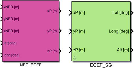
The software implementation of the position and velocity estimation algorithm follows a systematic approach. Each step mentioned above will be represented by a specific block, which reveals the underlying mathematical relationships and includes a user interface for inputting initial data (Figure 14).

Figure 14.

‘NED_ECEF’ and ‘ECEF_SG’ conversion blocks.

The integration block utilizes the initial values of speeds in the NED frame, the initial altitude, and the integration step [23].

The correction block requires latitude and altitude information obtained during the preceding iteration and applies the corrective model at each step (Figure 15) [22].

Figure 15.

MATLAB/Simulink scheme of the strap-down navigation algorithm.

Additionally, the NED → ECEF and ECEF→SG conversion blocks utilize for the current step the geodetic coordinates obtained before for accurate processing. They were also implemented according to [23].

The final scheme of the whole navigation algorithm, combining both attitude and global positioning parts can be observed in Figure 15. The subsystem ‘NAV’ that uses the IMU measurements and returns the attitude, position and velocity of the monitored vehicle was created from it in Figure 16.

Figure 16.

‘NAV’ simplified block of the navigation algorithm.

6. Validation of the wavelet filter and strap-down navigation algorithm integration

6.1 Flight scenario definition

The focus of this chapter is on the strap-down navigation system designed for deployment on aerial vehicles engaged in short-duration missions. Consequently, in the software-based experimental phase, the emphasis is placed on simulating real-life scenarios. Reference [12] serves as compelling evidence that the investigation of digital methods to optimize inertial sensor data is most effectively conducted by applying them in practical scenarios and analyzing their impact on the ultimate attitude and position results. To ensure this, specific constant acceleration and angular rate inputs have been selected for our study to mimic the conditions experienced during take-off and level-flight ascent: f_x = 5 m/s², f_y = 0 m/s², f_z = −9.82 m/s², om_x = om_z = 0^°/s, om_y = 0.2^°/s. The algorithm was also initalized with the following variables: v_N = 4 m/s, v_E = 0 m/s, v_D = −2 m/s, φ₀ = θ₀ = ψ₀ = 0. The starting point of the vehicle was set to 25.457319^° longitude, 44.926899^° latitude, and 20 m altitude. The duration of the mission (or the simulation time) was established to 60 seconds.

Observations:

• the z-axis specific force value was determined using the initial geodetic parameters, employing the relationship (16);

• initial attitude angles equal to 0 imply that the body-fixed frame is aligned with the NED frame;

• according to the initial NED speed components, the output latitude should encounter a slight rise, the longitude should remain close to zero and the altitude should significantly increase.

6.2 Generation of IMU perturbed data

To generate the perturbed MEMS outputs, referred to as “real” data, the aforementioned constant inputs were fed into the Simulink “IMU” block through the two MEMS models earlier mentioned and configured. The resulting signals from the simulation have been depicted in Figure 17.

Figure 17.

Perturbed IMU outputs: Accelerations – Left, angular speeds – Right.

The wavelet function chosen for denoising was Daubechies due to the previous results, and a 6-level decomposition was applied, resulting in the filtered signals shown in Figure 18.

Figure 18.

Filtered IMU outputs: Accelerations – Left, angular speeds – Right.

6.3 Simulation detection cases

The proper evaluation of the filter’s effectiveness involved conducting a numerical simulation in three distinct cases based on the type of inputs used for the algorithm in Simulink:

• Ideal Case: The ‘NAV’ block uses constant sensor inputs, representing the numerical values defined in the first section.

• Real/Perturbed Case: The ‘NAV’ block employs the perturbed inputs defined in Figure 17, applying numerical values at the entrance of the sensor models.

• Filtered Case: The ‘NAV’ block utilizes the filtered inputs defined in Figure 18, obtained by denoising the outputs shown in Figure 17.

Figure 19 presents the MATLAB/Simulink implementation of the three simulation cases.

Figure 19.

MATLAB/Simulink configuration of the three algorithm scenarios.

6.4 Results of the numerical simulation

The evaluation entailed comparing the absolute errors between the nine parameters (latitude, longitude, altitude, speed components in NED, and attitude angles) obtained from both the perturbed and filtered cases and the ideal navigation solution, which was illustrated in Figure 20. The evolution of the parameters follows the expected pattern from the picked numerical values:

• λ remains constant, Φ slightly increases, while h rises to almost 700 m from the initial value of 20 m;

• v_N increases, v_E remains null and v_D decreases;

• φ and ψ remain null, while θ increases to almost 12°.

Figure 20.

Ideal navigation solution.

Figure 21 shows the graphical representation of the errors obtained in both cases: red color for the perturbed case and blue color for the filtered case.

Figure 21.

Absolute errors obtained during the simulation.

Right from the outset, it becomes evident that the error curve of the filtered case exhibits a less pronounced trend compared to the perturbed case. This visual observation suggests that the filtering procedure enhances the error evolution in relation to the ideal navigation solution. In terms of numerical analysis, Table 4 presents the maximum absolute error values obtained for each parameter and input case.

Model	Maximum absolute error
	λ [deg] ·10^−4	Φ [deg] ·10^−4	h [m]	vN [m/s]	vE [m/s]	vD [m/s]	φ [deg] ·10^−3	θ [deg]	ψ [deg] ·10^−3
Perturbed	9.56	9.09	74.65	3.42	0.68	0.87	17.64	0.04	18.02
Filtered	2.18	8.47	16.78	3.18	0.58	0.83	2.76	0.02	5.01

Table 4.

Maximum absolute errors obtained during the simulation.

In every parameter case, the errors consistently decrease after filtration. Notably, the most significant improvement was observed in the altitude parameter, which saw a reduction of nearly 60 meters following wavelet denoising. Additionally, the attitude angles exhibit a clear enhancement in signal characteristics, effectively alleviating the oscillatory noise introduced to the output signal of the MEMS sensors. The overall performance of the wavelet filter proves to be notably high, demonstrating a clear improvement in the positioning accuracy of the monitored vehicle.

7. Conclusions

The chapter presented a modern approach on improving the measurements of low-cost miniaturized inertial sensors, which currently stand as a viable technical avenue for the architecture of inertial measurement units. These sensors can be seamlessly incorporated into the framework of strap-down inertial navigation systems, catering to diverse applications like aerial vehicle surveillance. Consequently, the precision and positioning accuracy of these sensors emerge as crucial focal points for researchers to enhance.

The primary aim of this study was to evaluate the applicability of wavelets, a potent analytical tool, in addressing the challenge posed by perturbed navigation data in strap-down MEMS IMUs.

Our research was divided into two distinct phases. The initial phase encompassed a comprehensive exposition of miniaturized inertial sensors and their typical errors. Subsequently, the issue of signal corruption associated with these sensors was outlined, along with the prerequisites for its resolution. The theoretical foundation of wavelet theory was introduced, accompanied by an enumeration of key reasons that render it a suitable choice for the present case.

The first experimental part involved an examination of the wavelet filter’s impact on an accelerometer and gyro model, both realized within MATLAB/Simulink. Distinct functions were employed for each sensor, and their efficacy was gauged through the computation of evaluation metrics. Following the application of the denoising technique using the MATLAB/Wavelet Analyzer tool, there was a notable reduction in noise levels, leading to enhanced signal attributes.

The second phase aimed at globally validating the efficacy of the wavelet filter by applying it to the complete strap-down navigation algorithm. The mathematical formulations of both attitude determination and position and velocity estimation components of the navigation algorithm were outlined, followed by their software implementation within MATLAB/Simulink. A practical scenario depicting the take-off of an aerial monitored vehicle was selected for numerical simulation of the strap-down algorithm. In this instance, to assess the performance of the denoising technique, three distinct input cases for the algorithm were examined. The ultimate objective was to compare the influence of unfiltered and filtered measurements on the navigation computation. Through a comparison of the absolute errors acquired in these two scenarios with the hypothetical ideal navigation solution, wherein numerical values serve as inputs, the outcomes underscored a substantial enhancement in positioning accuracy achieved through wavelet filtering. The evidence is presented through both graphical depictions and numerical values of the maximum absolute errors.

The overall conclusion drawn from the work presented in this chapter uncovers the potency of wavelets as a signal processing tool, offering remarkable attributes that hold promise for further advancements in the realm of MEMS-based strap-down INS. Given the numerous advantages bestowed by MEMS technology on the sensor market, the incorporation of wavelet filtering stands as a potentially advantageous step that could yield even greater benefits. The synergy between these two domains presents a compelling proposition that merits careful consideration and exploration.

References

1.Salychev O. Inertial Systems in Navigation and Geophysics. Moscow: Bauman MSTU Press; 1998
2.Ramalingam R, Anitha G, Shanmugam J. Microelectromechnical systems inertial measurement unit error modelling and error analysis for low-cost strapdown inertial navigation system. Defence Science Journal. 2009;59:650-658
3.Edu IR, Adochiei FC, Obreja R, Rotaru C, Grigorie TL. New tuning method of the wavelet function for inertial sensor signals denoising. In: CSCC ’14, Santorini Island, Greece, July 17-21, 2014. 2014
4.Al Bassam N, Ramachandran V, Eratt PS. Wavelet theory and application in communication and signal processing. In: Wavelet Theory. London, UK: IntechOpen; 2021. DOI: 10.5772/intechopen.95047
5.Pupo BL. Characterization of Errors and Noises in MEMS Inertial Sensors Using Allan Variance Method [Thesis]. Spain: Universitat Politècnica de Catalunya Barcelona Tech – UPC; 2016
6.Grigorie TL, Lungu R. Traductoare Accelerometrice și Girometrice. Craiova: Sitech; 2005
7.Nassar S, El-Sheimy N. Wavelet analysis for improving INS and INS/DGPS navigation accuracy. Journal of Navigation. 2005;58:119-134
8.Wirsing K. Time frequency analysis of wavelet and Fourier transform. In: Wavelet Theory. London, UK: IntechOpen; 2021. DOI: 10.5772/intechopen.94521
9.Hasan AM, Samsudin K, Ramli AR, Azmir RS. Wavelet-based pre-filtering for low cost inertial sensors. Journal of Applied Science. 2010;10:2217-2230
10.Ismaeel S, Al-Khazraji A. Wavelet decomposition for Denoising GPS/INS outputs in vehicular navigation system. WSEAS Transactions on Systems. 2017;16:197-203
11.Iontchev E, Miletiev R, Kapanakov P, Hristov L. Wavelet Algorithm for Denoising MEMS Sensor Data. Ohrid, North Macedonia: ICEST; 2019
12.Arya SJ, Jisha VR, Usha PMK. Implementation and performance assessment of wavelet Prefiltered platform tilt computation using low-cost MEMS IMU. In: 2022 IEEE 1st International Conference on Data, Decision and Systems (ICDDS), Bangalore, India. Vol. 2. IEEE; 2022
13.Song Q, Ma L, Cao J, et al. Image Denoising based on mean filter and wavelet transform. In: 2015 4th International Conference on Advanced Information Technology and Sensor Application (AITS). Epub ahead of print August 2015. 2015. DOI: 10.1109/aits.2015.17
14.IEEE Standard for Inertial Sensor Terminology. IEEE Std 528–2001. IEEE Standard for Inertial Sensor Terminology; 2001. pp. 1-26
15.Devices A. ADXRS150 ±150°/s Single Chip Yaw Rate Gyro with Signal Conditioning, Technical Datasheet. Analog Devices, Inc; 2004. pp. 1-12
16.Silicon Designs, Inc. S1221x-025 Single-Axis Accelerometer, Technical Datasheet. Silicon Designs, Inc.; 2006. pp. 1-16
17.Bayer FM, Kozakevicius AJ, Cintra RJ. An iterative wavelet threshold for signal denoising. Signal Processing. 2019;162:10-20
19.Grigorie TL, Sandu DG. On the attitude errors when the quaternionic Wilcox method is used. In: ELMAR 2007. Epub ahead of print September 2007. 2007. DOI: 10.1109/elmar.2007.4418804
20.Farrell J, Barth M. The Global Positioning System and Inertial Navigation. New York: McGraw-Hill Education; 1999
21.Dahia K. Nouvelles méthodes en filtrage particulaire: application au recalage de navigation inertielle par mesures altimétriques. 2005
22.Grigorie TL. Echipamente de Bord și Navigație Aeriană–Îndrumar de laborator. Craiova: Sitech; 2013
23.Grigorie TL, Sandu DG. Arhitecturi sinergice de sisteme de navigație cu componente inerțiale strap-down. Craiova: Sitech; 2013
Written By
Bianca-Gabriela Antofie, Marius-Ciprian Larco and Teodor Lucian Grigorie
Submitted: 09 August 2023Reviewed: 07 September 2023Published: 21 November 2023
Open access peer-reviewed chapter