Discrete Wavelet Transform Application to Three-Phase Power System Short Circuit Fault Detection

Abstract

In power system distribution, the transmission line is the bottleneck between power generation and consumers. Therefore, any fault or failure in the transmission line is critical and must be detected in a very short time. Meanwhile, as Discrete Wavelet Transform has special characteristics, it can be implemented to analyze and detect short circuit faults for the three-phase power system transmission line and identify the types based on phase-to-phase and phase-to-ground faults analysis. In this work, MATLAB Simulink was used to generate faults using a power distribution system simulator. The three-phase currents were analyzed using the Discrete Wavelet transform algorithm by decomposing the three-phase and ground currents and obtaining the detailed coefficients. As a result, the maximum value of the detailed coefficients is used to distinguish between different types of faults. Simulation results of the proposed method have shown promising results in detecting short circuit faults and identifying types of faults effectively.

1. Introduction

In the early days of ac power transmission in the United States, the operating voltage increased rapidly. Until 1917, electric systems were usually operated as individual units because they started as isolated systems and spread out only gradually to cover the whole country. The demand for large blocks of power and increased reliability suggested the interconnection of neighboring systems. Interconnection is advantageous economically because fewer machines are required as a reserve for operation at peak loads and fewer machines running without load are required to take care of sudden, unexpected jumps in load. Reducing machines is possible because one company usually calls on neighboring companies for additional power. Interconnection also allows a company to take advantage of the most economical sources of power, and a company may find it cheaper to buy some power than to use only its own generation during some periods. Interconnection has increased to the point where power is exchanged between the systems of different companies as a matter of routine.

Systems interconnection brought many new problems, most of which have been solved satisfactorily. Interconnection increases the amount of current that flows when a short circuit occurs on a system and required the installation of breakers to interrupt a larger current. The disturbance caused by a short circuit on one system may spread to interconnected systems unless proper relays and circuit breakers are provided at the interconnection point. Not only must the interconnected systems have the same nominal frequency, but also the synchronous generators of one system must remain in step with the synchronous generators of all the interconnected systems. Planning the operation, improvement, and expansion of the power system requires load studies, fault calculations, the design of means of protecting the system against lightning and switching surges and against short circuits, and studies of the system’s stability. Faults can be destructive to power systems. A great deal of study, development of devices, and design of protection schemes have resulted in continual improvement in the prevention of damages to transmission lines and equipment and interruption in generation following the occurrence of a fault.

With today’s advanced technology and widespread population across the globe, electrical power system networks become more complex to meet the growth in demand for electrical power energy. As a result, transmission lines can be seen as the arteries of the power system network that expand over several miles and act as an interconnection between power stations and consumers. Meanwhile, environmental effects on the open space transmission lines could cause fault occurrences in the power system [1]. In normal businesses operation and daily tasks, people’s lives are seriously affected by the fault of the power system. Whenever a fault occurs in the power system it causes damage to the devices connected and affects power quality transfer, power safety, and power stability that could lead to power blackouts [2].

Power transmission line fault identification and classification require fast and accurate analysis to detect the fault [3, 4]. The ability to detect and diagnose faults can help greatly in the protection of transmission lines and prevent damage to the power system. To solve this problem, a fault detection algorithm based on discrete Wavelet transform (DWT) is proposed in this paper. As power systems disturbances occurrence are nonstationary, nonperiodic, and short duration in most cases impulse super-imposed in nature, Wavelet transform can be one of the most suitable tools for the analysis of such faults and disturbances as in [3, 5, 6, 7]. The name wavelet first appeared in 1909 in thesis by Alfred Haar. Jean Morlet proposed the present theoretical form. The growth of interest in wavelets became huge. Wavelet analysis have developed mainly by Y. Meyer, and the main algorithm developed by Stephane Mallat in 1988. Since then many mathematicians and scientists have contributed towards the wavelets and their applications.

The main goal of this project is to find an accurate and quick way to detect short circuit fault to minimize system damage or even prevent it by taking action right away when fault detected. The process starts by generating known faults at known time using Simulink and MATLAB. The continuous wavelet transform is used to extract the detailed coefficients then compared it with a set threshold to detect if there is a fault then identify the fault type.

Per the IEEE 1159 standards, and as shown in [8, 9], constant observation for power system fault detection is required at all times to guarantee system reliability. Therefore, many researchers have studied power systems generation and distribution in terms of detecting faults and improving efficiency [10, 11, 12, 13, 14]. In [8, 15], about 70% of blackouts can be associated with power relay malfunction, which allows faulty tripping. Several loads are extremely sensitive to voltage sags, and several studies have investigated power relay setting by synchronizing delay and islanding [1]. Yet, a slower delay setting may cause serious load damage and fast tripping will cause excessive load isolation and shedding [2]. Meanwhile, other works had proposed monitoring the power system through Wide Area Monitoring (WAM) technique as in [16, 17]. Yet, it was observed by [18], that this technique requires a high-speed primary relay and sophisticated communication infrastructure [15]. In addition, other work focused on current/voltage waveform distortion caused by harmonics and surrounding noises. That is due to noise attenuation in the transmission line, the power relay was prepared with a harmonic controller surpassing 15% of the fundamental waveform. Thus, for larger fundamental waveforms, harmonics components may be added to the waveform without detecting faults. Meanwhile, some work has been done in the Wavelet transform decomposition process to vanquish conventional algorithms of current/voltage waveform analysis [2]. Therefore, to improve the exactness of monitoring the power system, this work will investigate the advantage of Wavelet transform in defining, locating, and classifying abnormality malfunction within a three-phase power system short circuit.

2. Wavelet and wavelet transform

Wavelets are mathematical functions derived from a mother wavelet. They are constructed by dilations and translations of the mother wavelet. The scaling parameter ‘a’ controls the dilation (expansion or contraction) of the wavelet, and the shift parameter ‘τ’ controls its translation along the time axis. This equation is showing the relationship between these parameters: ψ^{a, τ} (t) = |a|^−1/2ψ {(t - τ)/a}. The mother wavelet ψ is a function with a mean value of zero, i.e., its integral over all values of ‘t’ is equal to zero (∫ψ(t)dt = 0). The wavelet transform of a signal f(t) includes decomposing the signal into a group of basic functions (wavelets) with different scales and translations. This decomposition permits for representing the signal in terms of its different frequency components at various resolutions. The wavelet transform is suitable to use for both continuous-time and discrete-time signals. When the wavelet transform is applied on a signal, the scale components that represent the signal’s different frequency components at different scales. Low frequency wavelets have ‘a’ value greater than 1, which represent the larger time scales, while high-frequency wavelets have ‘a’ values less than 1, representing smaller time scales.

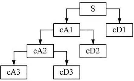
Wavelets have found numerous applications across various domains due to their ability to analyze and represent signals efficiently such as signal analysis, power system analysis, medical imaging, and other significant fields of functionalities [2, 4, 5]. The tree of wavelet decomposition is in Figure 1. The cA1, cA2 and cA3 are the approximation levels. The cD1, cD2 and cD3 are the detail levels while S is the signal of interest.

Figure 1.

Wavelet decomposition tree.

3. System design and modeling

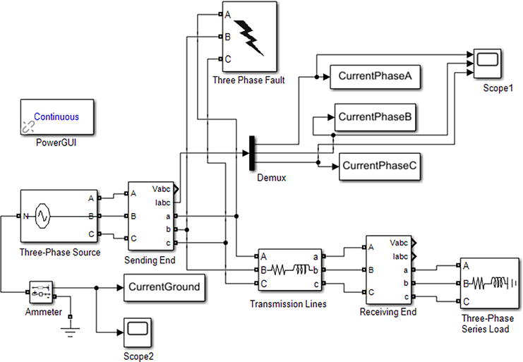
In this work of the new proposed algorithm to detect power transmission line fault, current signals under normal conditions (no fault) and the short circuit fault current signals are obtained to analyze and find a suitable detection and identification algorithm using wavelets transform. A power system simulation model was modeled using MATLAB/Simulink, as shown in Figure 2, to create and capture faults. The system is consisting of a three-phase source (generator), three-phase voltage-current measuring elements, transmission lines, current measuring (ammeter), scopes, load, and three-phase fault generators. The power system simulation model has a voltage level of 250 kV and a power frequency of 60 Hz. The three-phase power system is analyzed to examine its sustainability during fault experience. Short circuit faults such as single-phase-to-ground, multi-phase-to-ground, phase-to-phase, and three-phase faults are discussed. Both symmetrical and unsymmetrical faults are analyzed. The system can simulate all kinds of short-circuit faults that may occur in the power system.

Figure 2.

Power system simulation using MATLAB Simulink.

The three-phase source generates a sinusoidal signal with a frequency of 60 HZ. It is a balanced source with 120 degrees out of phase with each other. The internal connection is ‘Yn’ connection, which means the three voltage sources are connected in Y configuration and the neutral line is connected to the ground. The three-phase series RL branch block parameters represent the three-phase transmission lines.

One three-phase V-I measurement block parameter is used at the sending end. The block allows voltage and current measurements of all three phases to be taken simultaneously. The three inputs for the block at the sending end are the three phases of the generator, while the three inputs for the block at the receiving end are the three phases of the transmission lines.

For fault identification, all three phase current measurements as well as neutral current measurements are required [19]. Therefore, the de-multiplexer (Demux) block is used to separate all the three-phase currents. PowerGui (continuous simulation) block is used to simulate the Simulink model that contains electrical specialized power systems blocks. PowerGui is a required block to implement the functions within the toolbox.

Current signals of each phase are recorded in MATLAB workspace to apply DWT on these current signals for fault detection and diagnosis and they are labeled as CurrentPhaseA, CurrentPhaseB, and CurrentPhaseC to represent the three-phase currents A, B, and C. To distinguish between line (phase) to line (phase) fault and double line to ground fault, neutral current is measured. Ammeter is used to measure and transfer the neutral current to the workspace using the ‘To workspace” block and labeled as (Current Ground). The scope is used to display the three-phase voltages and the three-phase currents.

The three-phase fault block parameters are used to implement a fault (short-circuit) between any phase and the ground. The fault timing is defined directly from the dialog box in this project simulation. Replace the entirety of this text with the main body of your chapter. The body is where the author explains experiments, presents and interprets data of one’s research. Authors are free to decide how the main body will be structured. However, you are required to have at least one heading. Please ensure that either British or American English is used consistently in your chapter.

4. Proposed algorithm

We combine the characteristics of the fault signal and the detection algorithm based on Wavelet transform as follows:

• Simulink is used to build the power system model.

• The three-phase current signals are obtained.

• The Mother Wavelet (Daubechies-4) is used to extract the approximation and detailed coefficients for level one.

• The threshold value is set.

• The maximum values of the detailed coefficients are obtained.

• The detailed coefficients’ maximum values are compared with the threshold (Td).

• Faults detect if the maximum values of the detailed coefficients are larger than the threshold.

• Then, the fault type is identified.

To start, the fault was created using the block parameters-three phase faults at 0.05 seconds and remove the fault at 0.1 seconds. Discrete Wavelet transform is used since it is an effective tool for analyzing the current signals. The current signals are decomposed using Daubechies Wavelet-4 (db4) to obtain the approximate and detailed coefficients at level one. Then the decomposed signals are used for the detection of faults by using the detailed coefficients.

To distinguish between different types of faults, the maximum value of the current signal must be defined by measuring the maximum value of all coefficients for phase A, phase B, phase C, and the ground current as shown in Table 1. By setting the parameters of the three-phase fault block parameters, the three-phase current of the detailed coefficients of phase A, phase B, phase C, and ground current.

Case No.	Maximum Detailed Coefficient Of Phase A Current	Maximum Detailed Coefficient Of Phase B Current	Maximum Detailed Coefficient Of Phase C Current	Maximum Detailed Coefficient Of Ground Current	Fault Type
1	103.9844	103.9844	103.9844	7.8793e-10	No Fault
2	1.3523e+06	103.9844	119.5264	1.6087e+06	Line to Ground (A-G)
3	103.9857	3.7024e+06	134.4171	1.1253e+06	Line to Ground (B-G)
4	103.9857	103.9844	1.4099e+06	1.4099e+06	Line to Ground (C-G)
5	3.6468e+07	1.2349e+07	104.6234	.0454	Line to Line (A-B)
6	2.1185e+07	111.4911	4.9922e+07	0.0146	Line to Line (A-C)
7	104.6286	3.1411e+07	8.6390e+07	0.0101	Line to Line (B-C)
8	1.0667e+07	2.1332e+07	119.5264	7.7120e+05	Double Line to Ground (AB-G)
9	1.9807e+07	103.9844	8.6994e+06	1.9393e+06	Double Line to Ground (AC-G)
10	103.9857	4.0725e+07	8.4664e+06	9.7973e+05	Double Line to Ground (BC-G)
11	1.2506e+07	2.9173e+07	9.0875e+07	0.0065	Three Phase Fault

Table 1.

Maximum value of detailed coefficients of all phases and ground current for different faults.

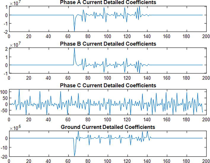
The detailed coefficients in the phase that has a fault will have a high value while the coefficients in the other phases that have no fault will have zero magnitudes or very small values. This means when there is no fault in the power system, the value of the coefficients in all phases is zero or very small. The threshold value needs to set in order to distinguish between the fault types. If the highest value for the detailed coefficient for any current signal is above that threshold, then that line (phase) has a fault. The no-fault value is the threshold value, and all other values are with different faulty conditions. This way, we can distinguish between different types of faults.

As an example, when we apply two phases (phase A and phase B) to ground fault (AB-G) in the power system and measure the maximum value of all the coefficients, phase A, phase B, and ground currents have a very high value of the coefficient, while phase C has a very small value of confidence. The results of the applying system and the ground current can be extracted through Scope1 and Scope2.

5. Fault detection using wavelet transform

The three-phase power system’s currents and voltages are sinusoidal signals when there is no fault. A fault in the power system causes changes in the current and voltage signals [19]. A short circuit fault occurs in the transmission lines, current signals will have transient components [19]. Meanwhile, as Wavelet transform analyzes a localized area of signal and provides information like breakpoints and discontinuities, Wavelet transform can be very useful in detecting the start of the fault and realizing non-stationary signals including both low and high-frequency components [6]. The first level of decomposition contains high frequencies that are associated with the faults. Fault detection can be obtained by examining the detailed coefficients of the first-level decomposition of the current signal.

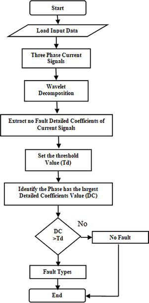
When the transient components are presence then the fault is detected by comparing the current detailed coefficients with the threshold. If the value is larger than the Td, then there is a fault as presented in the flowchart block diagram algorithm of Figure 3. The wavelet transform is applied to the three-phase current A, B, C, and the ground current G for decomposition which provide the detailed coefficients and the approximation coefficients using Daubechies Wavelet-4 (db4) stage one decomposition. By comparing the absolute maximum value of each phase detailed coefficients to the Td, the presence of the fault can be determined. There is fault in a phase when the value for that phase’s detailed coefficients is larger than the Td. Then the type of the fault is identified by exposing the faulty phase to further analysis. In this paper, the value of Td is choosing to equal 175. If the value of the coefficient for phase current is less than the Td, there is no fault, and the system is operating in normal healthy condition. If the value of the detailed coefficient for any phase current exceeds the Td value, then the fault type can be identified.

Figure 3.

The flowchart for short circuit fault detection.

6. Fault type and discussion

The Wavelet used in this project is db4 with first-level decomposition. By comparing the three-phase current and the ground current detailed coefficients with a threshold, we can capture the fault and determine the type of all faults. Since the faulty phase detailed coefficients (absolute maximum value) is larger than the threshold, using the proposed algorithm we detect all faulty lines and determine the fault types.

This method allows distinguishing and determining all type of faults:

1. Symmetrical Fault (Balanced Fault):

• Three phase fault (LLL).

• Three phase to ground fault (LLLG).

1. Unsymmetrical Faults (Unbalanced Faults):

• Single phase to ground fault (LG).

• Two phase fault (LL).

• Two phase to ground fault (LLG)

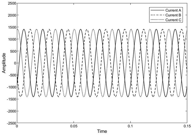
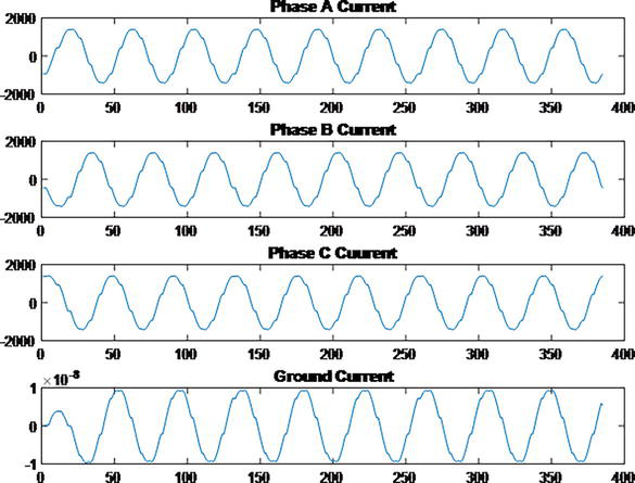
From Table 1, it was noticed that all types of faults’ coefficient values were extremely high, while for no fault applied in any of the phases, the value was very small as shown in Figure 4 for the three-phase current with no fault embedded. Meanwhile, to illustrate the finding in faulty three-phase current, five different faults were captured and displayed including the approximation and the detailed coefficients as shown in Figures 5–27.

Figure 4.

Simulink no fault three-phase current.

Figure 5.

Algorithm no fault three-phase current.

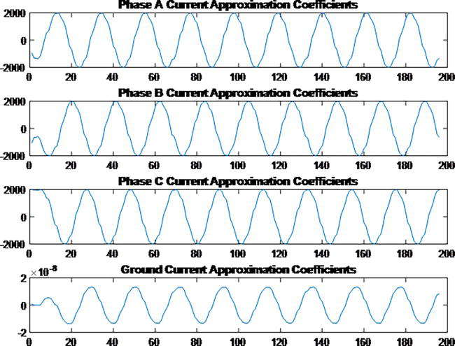
Figure 6.

Three phase current approximation coefficients.

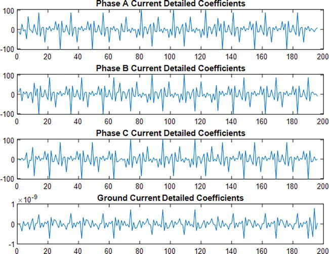
Figure 7.

Algorithm no fault three-phase current detailed coefficients.

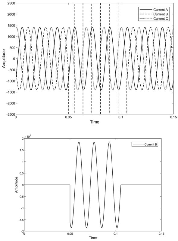
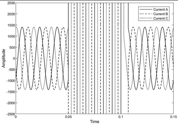
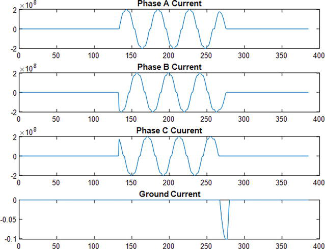
Figure 8.

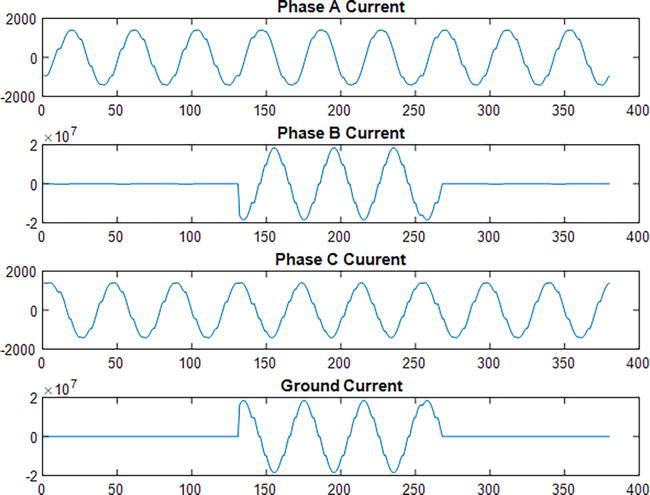
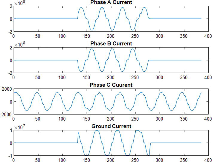
Simulink current phase B to ground fault (B-G).

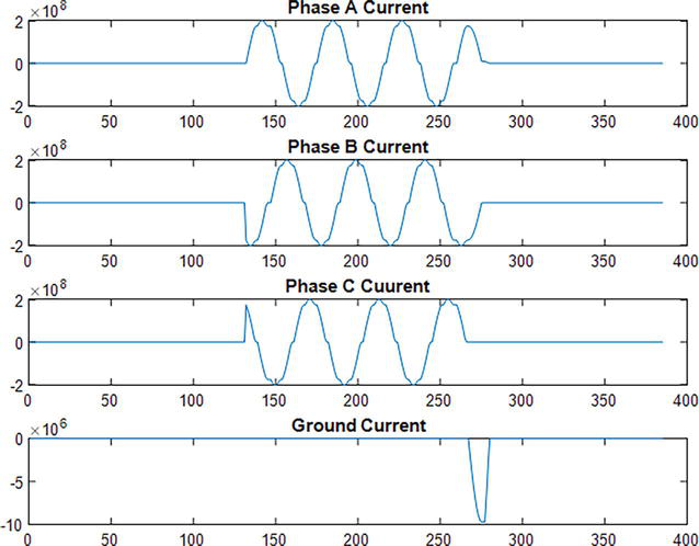
Figure 9.

Algorithm single phase B to ground fault.

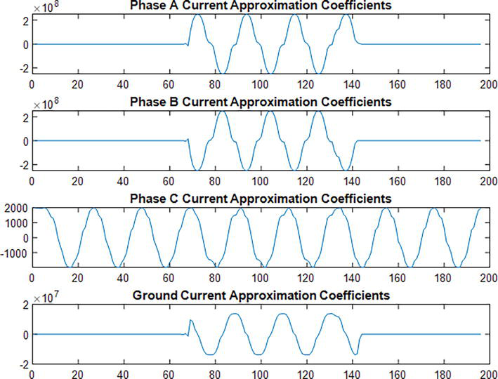
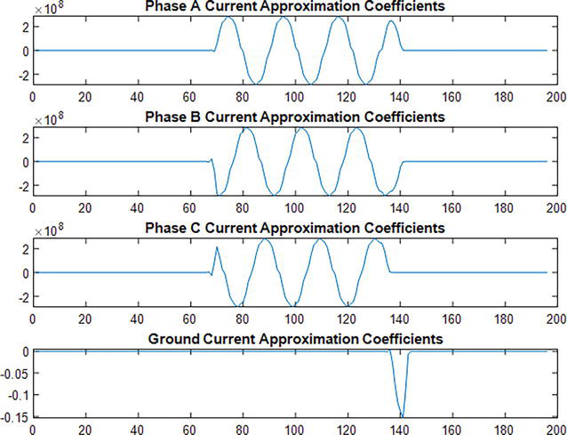
Figure 10.

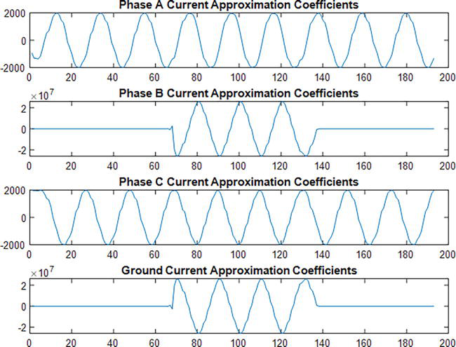
Single phase B to ground fault approximation coefficients.

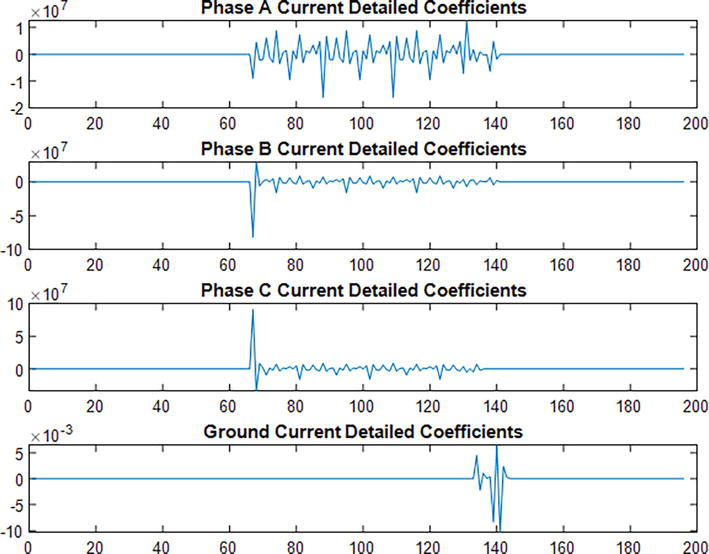
Figure 11.

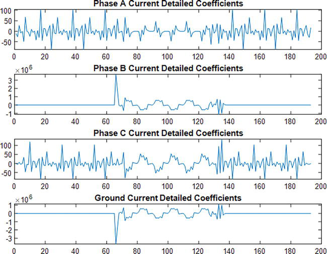
Single phase B to ground detailed coefficients.

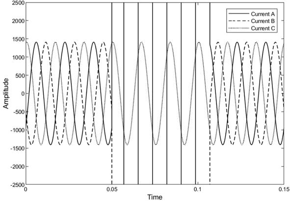
Figure 12.

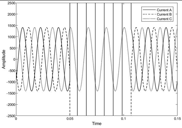
Simulink double phase fault – Phase a to phase B fault.

Figure 13.

Algorithm double phase fault (phase a to phase B fault).

Figure 14.

Double phase fault (phase a to phase B fault) approximation coefficients.

Figure 15.

Double phase fault (phase a to phase B fault) detailed coefficients.

Figure 16.

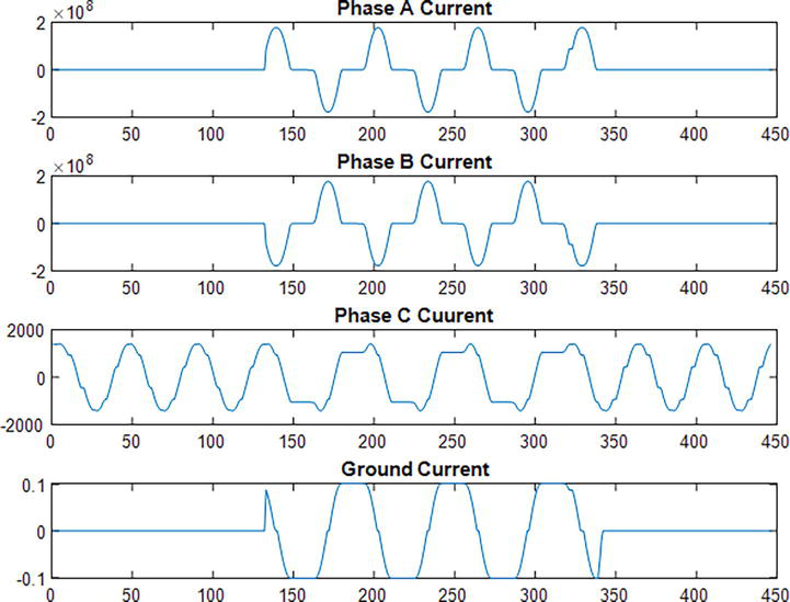
Simulink double phase to ground fault (AB-G).

Figure 17.

Algorithm double phase to ground fault (AB-G).

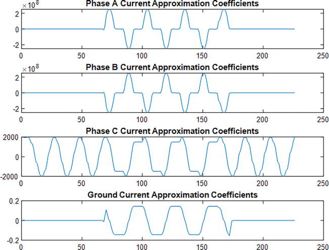
Figure 18.

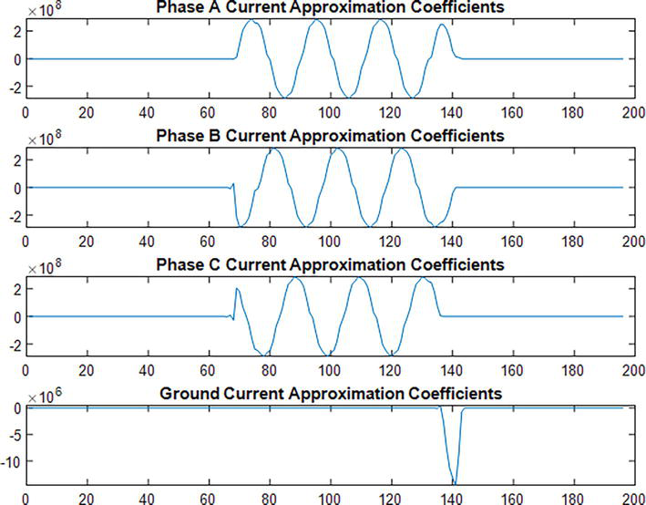
Double phase to ground fault (AB-G) approximation coefficients.

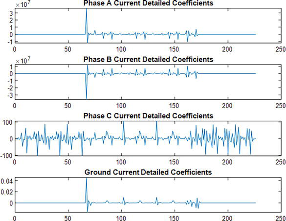
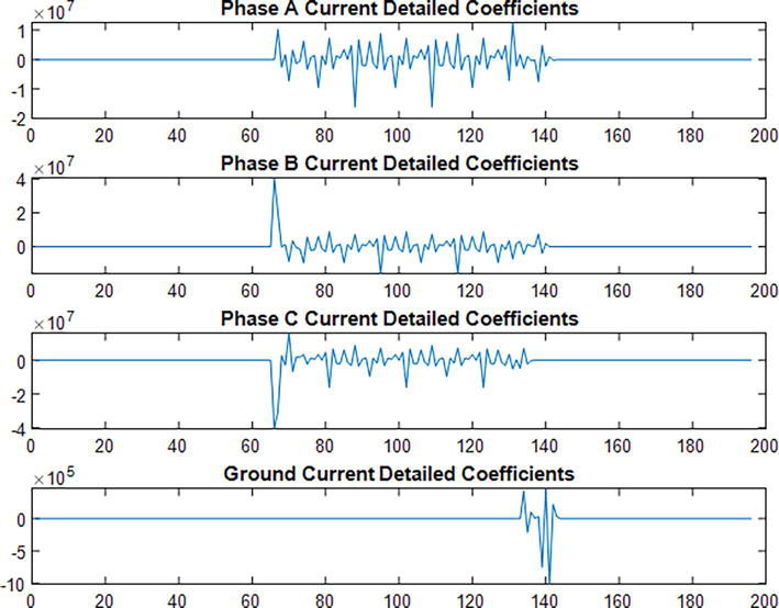
Figure 19.

Double phase to ground fault (AB-G) detailed coefficients.

Figure 20.

Simulink three-phase fault (ABC).

Figure 21.

Algorithm three-phase fault (ABC).

Figure 22.

Algorithm three-phase fault (ABC) approximation coefficients.

Figure 23.

Algorithm three-phase fault (ABC) detailed coefficients.

Figure 24.

Simulink three-phase to ground fault (ABC-G).

Figure 25.

Algorithm three-phase to ground fault current (ABC-G).

Figure 26.

Three-phase to ground fault (ABC-G) approximation coefficients.

Figure 27.

Three-phase to ground fault (ABC-G) detailed coefficients.

As an example, the case of the single phase to ground fault (B-G) illustrated in Figure 8, clearly shows abnormal phase B signal behavior when the fault is applied. When a fault occurs in a phase that phase’s current increases. Which is the same result occurred for all types of faults applied.

The table shows that the detailed coefficient values are extremely high for all types of faults while the detailed coefficient values are very small when there was no fault applied.

We can assign a value for the threshold by finding the largest value for all the maximum detailed coefficients for all phases with no fault (from Table 1. = 134.4171), then choose a reasonable larger value for the threshold such as Td = 175.

The three-phase current ABC and the ground under normal conditions (no fault) are illustrated in Figures 4–7 where the detailed coefficient values for all the currents are very small.

The single phase to ground fault (B-G) illustrated in 8–11 is clearly showing abnormal phase B signal behavior. The phase and ground current increased when the fault occur, and the maximum value of the detailed coefficients for phase B and ground currents have a very high value while phases A and C have a very small value of coefficients.

The two-phase fault (A-B) is illustrated in Figures 9–15 which shows abnormal phase A and phase B signal behavior. The two-phase currents increased when the fault occurs and the maximum value of the detailed coefficients for phase A, and phase B currents have a very high value while phase C and the ground have a very small value of coefficients.

The two phases to ground fault (AB-G) are illustrated in Figures 15–19, which shows abnormal phase A, and phase B signal behavior. The two-phase and ground current increased when the fault occurs and the maximum value of the detailed coefficients for phase A, phase B, and ground currents have a very high value while phase C has a very small value of coefficients.

The three-phase fault (ABC) is illustrated in Figures 20–23 which shows abnormal phase A, phase B, and phase C signal behavior. The three-phase current increases when the fault occurs and the maximum value of the detailed coefficients has a very high value while the ground current has a very small value of coefficients.

The three-phase to ground fault (ABC-G) is illustrated in Figures 24–27 which shows abnormal signal behavior in all phases and the ground. The three phases and the ground current increased when the fault occurs and the maximum value of the detailed coefficients for all have a very high value.

7. Conclusion

We have used wavelet transform successfully to detect and identify the short circuit fault in the power system. Different types of faults on the transmission lines are simulated by using MATLAB/Simulink. The current in each phase is recorded and the detailed coefficients of the first level decomposition are extracted using wavelet (db4). The no-fault detailed coefficients are obtained and compared with the threshold value of the system to detect and identify the fault. We observed that if the system has no fault, these values are less than the threshold value, while these values exceed the threshold values when there is a fault. The proposed algorithm is fast and accurate because it depends upon the detailed coefficients extracted from one stage and it achieves an accurate result under all short circuit fault types.

References

1.Asman SH, Ab Aziz NF, Ungku Amirulddin UA, Ab Kadir MZ. Transient fault detection and location in power distribution network: A review of current practices and challenges in Malaysia. Energies. 2021;14(11):2-20. DOI: 10.3390/en14112988
2.Awada E. Numerical voltage relay enhancement by integrated discrete wavelet transform. Journal of Southwest Jiaotong University. 2021;56(6):843-854. DOI: 10.35741/issn.0258-2724.56.6.74
3.Huang S-J, Hsieh C-T. Computation of continuous wavelet transform via a new wavelet function for visualization of power system disturbances. In: 2000 Power Engineering Society Summer Meeting (Cat. No.00CH37134). Vol. 2. Seatle, WA, USA: IEEE; 2000. pp. 951-955. DOI: 10.1109/PESS.2000.867500
4.Awada E, Radwan E, Nour M, Al-Qaisi A, Al-Rawashdeh AY. Modeling of power numerical relay digitizer harmonic testing in wavelet transform. Bulletin of Electrical Engineering and Informatics. 2023;12(2):659-667. DOI: 10.11591/eei.v12i2.4553
5.Akujuobi CM. Wavelets and Wavelet Transform Systems and their Applications:A Digital Signal Processing Approach. Switzerland: Springer; 2022. DOI: 10.1007/978-3-030-87528-2
6.Reddy BR, Kumar MV, Suryakalavathi M, Babu CP. Fault detection, classification and location on transmission lines using wavelet transform. In: 2009 IEEE Conference on Electrical Insulation and Dielectric Phenomena. Virginia Beach, VA, USA: IEEE; 2009. pp. 409-411. DOI: 10.1109/CEIDP.2009.5377788
7.Mishra R, Deoghare PM. Analysis of transmission line fault by using wavelet. International Journal of Engineering Research & Technology (IJERT). 2014;3(5):36-40
8.Abdelmoumene A, Bentarzi H. Reliability enhancement of power transformer protection system. Journal of Basic and Applied Scientific Research. 2012;10:10534-10539
9.Zbunjak Z, Kuzle I. System integrity protection scheme (SIPS) development and an optimal bus-splitting scheme supported by phasor measurement units (PMUs). Energies. 2019;12(17):1-12. DOI: 10.3390/en12173404
10.Akhmetova IG, Chichirova ND. The reliability and efficiency of power companies. In: SHS Web Conf. Vol. 35. 2017. p. 01108. DOI: 10.1051/shsconf/20173501108
11.Salawudeen AT, Olaniyan AA, Olarinoye GA, Sikiru TH. Formulation and Optimization of Overcurrent Relay Coordination in Distribution Networks Using Metaheuristic Algorithms. Vol. 1350. Minna, Nigerai: Springer International Publishing; 2021. DOI: 10.1007/978-3-030-69143-1_30
12.Irfan M et al. An optimized adaptive protection scheme for numerical and directional overcurrent relay coordination using Harris hawk optimization. Energies. 2021;14(18):1-11. DOI: 10.3390/en14185603
13.Hong L, Rizwan M, Rasool S, Gu Y. Optimal relay coordination with hybrid time–current–voltage characteristics for an active distribution network using alpha Harris hawks optimization. Engineering Proceedings. 2021;12(1):1-5. DOI: 10.3390/engproc2021012026
14.Ramli SP, Mokhlis H, Wong WR, Muhammad MA, Mansor NN, Hussain MH. Optimal coordination of directional overcurrent relay based on combination of improved particle swarm optimization and linear programming considering multiple characteristics curve. Turkish Journal of Electrical Engineering and Computer Sciences. 2021;29(3):1765-1780. DOI: 10.3906/elk-2008-23
15.Phadke AG, Wall P, Ding L, Terzija V. Improving the performance of power system protection using wide area monitoring systems. Journal of Modern Power Systems and Clean Energy. 2016;4(3):319-331. DOI: 10.1007/s40565-016-0211-x
16.Gadiraju HKV, Barry VR, Jain RK. Improved performance of PV water pumping system using dynamic ReconFigureuration algorithm under partial shading conditions. CPSS Transactions on Power Electronics and Applications. 2022;7(2):206-215. DOI: 10.24295/CPSSTPEA.2022.00019
17.Kalas A, Fauzy M, Dessouki ME, El-refay AM, El-zefery M. High performance direct torque control for induction motor drive fed from photovoltaic system. International Journal of Electrical, Computer, Energy, and Communication Engineering. 2015;9:11
18.Alawady AA, Alkhayyat A, Jubair MA, Hassan MH, Mostafa SA. Analyzing bit error rate of relay sensors selection in wireless cooperative communication systems. Bulletin of Electrical Engineering and Informatics. 2020;10(1):216-223. DOI: 10.11591/eei.v10i1.2492
19.Eldin ESMT. Fault location for a series compensated transmission line based on wavelet transform and an adaptive neuro-fuzzy inference system. In: Proceedings of the 2010 Electric Power Quality and Supply Reliability Conference. Kuressare, Estonia: IEEE; 2010. pp. 229-236. DOI: 10.1109/PQ.2010.5549994
Written By
Maysoun Alshrouf, Cajetan M. Akujuobi and Emad Awada
Submitted: 12 July 2023Reviewed: 19 July 2023Published: 08 October 2023
Open access peer-reviewed chapter