Application of Complex Hilbert Principal Component Analysis to the Economic Phenomena

Abstract

Conventional principal component analysis operates using a correlation matrix that is defined in the space of real numbers. This study introduces a novel method—complex Hilbert principal component analysis—which analyzes data using a correlation matrix defined in the space of complex numbers. As a practical application, we examine 10 major categories from the Japanese Family Income and Expenditure Survey for the period between January 1, 2000 and June 30, 2023, paying special attention to the time periods preceding and following the onset of the novel coronavirus disease 2019 pandemic. By analyzing the mode signal’s peaks, we identify specific days that exhibit characteristics that are consistent with the events occurring before and after the pandemic.

1. Introduction

The analysis of big data may reveal novel aspects of nature and of our society. However, the significance of datasets is often obscured by noise, so distinguishing meaningful signals from such noise is an essential task. Principal component analysis (PCA) is a valuable tool for understanding the characteristics of a dataset by reducing its dimensionality to fewer dimensions than exist in the original dataset. PCA has long been exploited in various fields of study ranging from natural science to the social sciences and was recently used with machine learning as a dimensionality reduction method.

A pioneering economic study that used PCA by Connor and Korajczyk [1] to derive factors from a large set of stock returns, which led to PCA’s application in various areas of economics from microeconomics to macroeconomics (e.g., [2, 3, 4, 5, 6, 7]).

PCA’s key point is to distinguish between significant and random components. The Scree criterion for factor retention introduced by Cattell [8] is useful for visually identifying the separation point. In statistical physics, the distribution of eigenvalues [9] and of components of corresponding eigenvectors [10] were derived analytically in research on random matrix theory (RMT). The authors from references [11, 12, 13] developed an RMT-based “null hypothesis” test that explicitly compares the properties of empirical equal-time cross-correlation matrices to those of random matrices. Any deviations from the properties of a random matrix were considered indicators of meaningful information. The RMT method has been applied to the equal-time cross-correlation matrix of assets [14, 15, 16, 17, 18, 19].

Plerou et al. [13] constructed a “filtered” cross-correlation matrix using eigenvalues and eigenvectors outside of the bounds of a random matrix and applied it to Markowitz’s portfolio optimization [20]. Their results showed that predicted risk is more closely aligned with realized risk when using a cross-correlation matrix than when using traditional portfolio optimization methods. The authors from references [21, 22] applied Markowitz’s portfolio optimization technique to stocks listed in the first division of the Tokyo Stock Exchange and demonstrated that the performance of portfolios constructed using this method generally outperformed market indices such as the Tokyo Price Index (TOPIX).

RMT is a robust technique for isolating the meaningful components from background noise in financial time-series data. The null hypothesis used in this method assumes both cross-correlation and autocorrelation randomness. However, autocorrelation in stock returns is generally not random, as evidenced by studies such as in Ref. [23]. Therefore, a new method that maintains autocorrelation while randomizing cross-correlation is required. To address this need, the authors from references [24, 25] introduced Rotational Random Shuffling (RRS), a method in which empirical time-series data are rotationally shuffled along the time axis, subject to periodic boundary conditions. Equal-time cross-correlation matrices generated from RRS time-series data preserve most of the autocorrelation while effectively randomizing the cross-correlation. A comparison between the eigenvalue distribution of the RRS-generated cross-correlation matrix and that of the empirical matrix enables one to effectively differentiate between meaningful components and noise.

Extending the application of RMT to cross-correlation matrices that consider different time frames was a natural development. Arai et al. [26] introduced complex Hilbert principal component analysis (CHPCA), in which the cross-correlation matrix is formulated in complex space, and the components of the eigenvectors are distributed across the complex plane, allowing for the identification of lead-lag relationships between components using angular differences. The authors from references [27, 28] applied CHPCA to a time-series dataset of assets in the S&P 500. Vodenska et al. [29] employed CHPCA to explore foreign exchange and stock market data from 48 countries for the 1990–2012 period and revealed significant lead-lag relationships between these markets. Souma et al. [30] used CHPCA to analyze a time-series dataset for assets listed on the New York Stock Exchange from 2005 to 2014, illuminating lead-lag relationships between stocks, investment trusts, real estate investment trusts, and exchange-traded funds. The authors from references [31, 32] applied CHPCA to the early warning indicators for a financial crisis proposed by the Bank of Japan to investigate shifts in the lead-lag relationships between indices before and after a financial crisis.

When applying CHPCA to time-series data, explicitly extracting the lead-lag relationships between the different time series is essential. The authors from references [33, 34, 35] employed the Helmholtz-Hodge decomposition (HHD) to identify circular and gradient flows within complex networks. Iyetomi [36] used CHPCA and HHD on monthly time-series data for 57 U.S. Macroeconomic indicators and five trade/money indices and statistically confirmed significant co-movement among these time series, pinpointing significant economic events. Iyetomi et al. [37] summarized CHPCA, RRS, and HHD and applied these methodologies to economic time-series data.

Souma et al. [38] investigated the complex interdependencies between the economic policy uncertainty (EPU) and geopolitical risk (GPR) indices across 31 countries by using CHPCA to identify key events that prompted significant changes in EPU and GPR index values for the 1997–2020 period and examining the leading and lagging relationships between countries to determine whether one country’s EPU or GPR index could influence those of another’s. This study demonstrated that CHPCA enables a weighted and directed network to be constructed from the correlation matrix and concluded that the most impactful event of this period was the September 11, 2001 terrorist attacks, followed by the COVID-19 pandemic in 2020 and the global financial crisis in 2008.

The objective of this chapter is to apply CHPCA to the Japanese Family Income and Expenditure Survey (FIES), which is conducted by the Statistics Bureau of Japan [39], and to clarify the characteristics of consumption before and after the COVID-19 pandemic. In Section 2, we describe the characteristics of the FIES data, which consists of daily consumption records extending from January 1, 2000 through June 30, 2023. We remove trends, seasonality, and weekly effects from this dataset. In Section 3, we outline the CHPCA methodology and discuss random shuffling (RS), RRS, and mode signals. In Section 4, we present our findings, demonstrating that CHPCA is able to successfully extract the characteristics of typical events occurring before and after the COVID-19 pandemic using consumption as the mode signal. Finally, Section 5 presents a summary and discussion.

2. Data

This chapter investigates the FIES conducted by the Statistics Bureau of Japan [39]. The FIES is a sample survey that includes households, excluding single-person student households. The 2015 Population Census covered 51.57 million households and represented 96.5% of all Japanese households. Sample households for the FIES are chosen using statistical methodologies that ensure that the FIES data may represent all households in the country. Approximately 9000 households were selected using a three-stage sampling method. Each sampled family household recorded its income and expenditure in a family account ledger for 6 months and for 3 months single-person households.

The FIES comprises multi-person households (i.e., those with two or more persons) and single-person households. Of the approximately 9000 households surveyed, about 85.7% are multi-person households, while approximately 14.3% are single-person households.

Although the proportion of single-person households has recently been increasing, this chapter focuses on data for multi-person households, as they remain the predominant type of Japanese household. The FIES began in September 1950, and census data starting in January 2000 can be downloaded from reference [40]. The number of disclosed items exceeds 150. There are 10 major consumption expenditure categories as follows: 1. Food, 2. Housing, 3. Fuel, light & water charges, 4. Furniture & household utensils, 5. Clothing & footwear, 6. Medical care, 7. Transportation & communication, 8. Education, 9. Culture & recreation, and 10. Other Consumption Expenditures.

While FIES reports and statistical tables are published monthly, they feature daily data, so this section delves into the characteristics of the daily data associated with the 10 primary consumption items. The dataset includes six leap years. To standardize each year to 365 days for this analysis, we compute the average consumption expenditures for February 28 and 29 and then assign this average to February 28. Then, we exclude February 29. We denote the consumption expenditure of the $n$-th item in year $y$ on day $d$ as $X_{n,y,d}$.

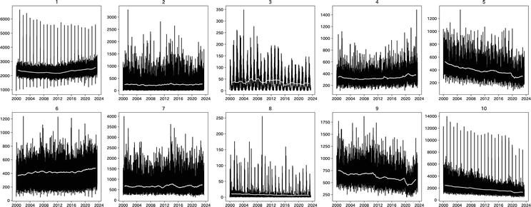
Figure 1 portrays the daily fluctuations of these 10 primary consumption items from January 1, 2000, to June 30, 2023. In this figure, each white line represents the one-year moving average, highlighting the existence of a trend. To remove the trend from each time series, we calculate the change relative to the corresponding day in the previous year using the following equation:

Figure 1.

Original data for 10 categories of the Japanese family income and expenditure survey. Source: The statistics Bureau of Japan.

$$R_{n,y,d}=\frac{X_{n,y,d}}{X_{n,y-1,d}}.$$E1

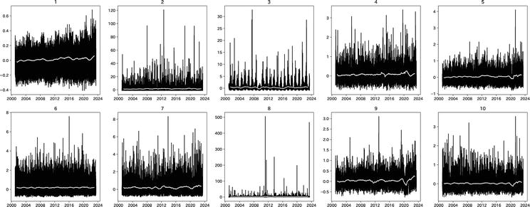
Hereafter, we will denote $R_{n,y,d}$ as $R_{n,t}$.The results of this transformation are illustrated in Figure 2. In this figure, each white line represents a one-year moving average of $R_{n,t}$, which highlights the existence of a trend denoted $G_{n,t}$.

Figure 2.

Change in 10 categories of the Japanese family income and expenditure survey from the same day the previous year.

In addition to the trend $G_{n,t}$, the time series $R_{n,t}$ contains seasonality $S_{n,t}$. To remove these components, we obtain the following equation:

$$Y_{n,t}=R_{n,t}-G_{n,t}-S_{n,t}.$$E2

However, $Y_{n,t}$ is still subject to day-of-the-week effects, $D_{n,t}$, defined as follows:

$$D_{n,t}=\frac{1}{N_d}\sum _{t\in d}{Y}_{n,t},$$E3

where $N_d$ represents the number of days in a week. Therefore, after removing $D_{n,t}$ from $Y_{n,t}$, we obtain the following:

$$r_{n,t}=Y_{n,t}-D_{n,d}.$$E4

The resulting time series passes both the Augmented Dickey-Fuller test and the Kwiatkowski-Phillips-Schmidt-Shin tests.

3. Methods and materials

In this section, we explain how CHPCA is used to explore the correlation structure of $r_{n,t}$.

3.1 Complex correlation matrix

The mean value of $r_{n,t}$ is defined as follows:

$$⟨r_n⟩=\frac{1}{T}\sum _{t=1}^T{r}_{n,t}.$$E5

The variance is given by the following:

$${\sigma }_n^2=\frac{1}{T}\sum _{t=1}^T{\left(r_{n,t}-⟨r_n⟩\right)}^2.$$E6

To standardize $r_{n,t}$, as defined in Eq. (4), to have a mean of zero and a variance of one, we use the following:

$$w_{n,t}=\frac{r_{n,t}-⟨r_n⟩}{{\sigma }_n}.$$E7

The Fourier transform of Eq. (7) is given as follows:

$$w_{n,t}=\sum _{k=0}^T\left[a_n\left({\omega }_k\right)cos\left({\omega }_{k}t\right)+b_n\left({\omega }_k\right)sin\left({\omega }_{k}t\right)\right],$$E8

where ${\omega }_k=2\mathit{\pi k}/T\ge 0$.

The Hilbert transform of Eq. (8) is given by the following:

$${\widehat{w}}_{n,t}=\sum _{k=0}^T\left[b_n\left({\omega }_k\right)cos\left({\omega }_{k}t\right)-a_n\left({\omega }_k\right)sin\left({\omega }_{k}t\right)\right].$$E9

Eq. (9) corresponds to Eq. (8) shifted to the phase $\pi /2$. Therefore, Eqs. (8) and (9) are orthogonal to each other. Now, using Eqs. (8) and (9), we define the complex time series as follows:

$${\tilde{w}}_{n,t}=w_{n,t}+i{\widehat{w}}_{n,t}=\sum _{k=0}^T{c}_n\left({\omega }_k\right)e^{-i{\omega }_{k}t},$$E10

where $i$ is an imaginary unit defined by $i^2=-1$, and $c_n\left({\omega }_k\right)=a_n\left({\omega }_k\right)+i{b}_n\left({\omega }_k\right)$.

The right-hand side of Eq. (10) indicates that ${\tilde{w}}_{n,t}$ rotates in a clockwise direction over time. The matrix with the components specified by Eq. (10) is known as the complex Wishart matrix, and it can be expressed as follows:

$$\tilde{\mathbf{W}}=\left[{\tilde{w}}_{n,t}\right].$$E11

Consequently, the complex correlation matrix is defined by the following:

$$\mathrm{C}=\frac{1}{T}{\tilde{\mathbf{W}}\tilde{\mathbf{W}}}^{†},$$E12

where ${\tilde{\mathbf{W}}}^{†}$ denotes the adjoint matrix of $\tilde{\mathbf{W}}$ (i.e., the transpose and complex conjugate).

The components of the complex correlation matrix can be expressed as follows:

$$C_{\mathit{mn}}=Re\left(C_{\mathit{mn}}\right)+iIm\left(C_{\mathit{mn}}\right),$$E13

$$=\left|C_{\mathit{mn}}\right|e^{i{\phi }_{\mathit{mn}}},$$E14

where ${\phi }_{\mathit{mn}}$ represents the correlation in phase space. The leading or lagging behavior of each component is determined using ${\phi }_{\mathit{mn}}$.

3.2 Random shuffling and rotational random shuffling

We can generate a random complex correlation matrix devoid of both autocorrelation and cross-correlation by employing a randomly shuffled Wishart matrix as follows:

$$w_{n,t}\to w_{n,rand\left[1,T\right]},$$E15

where $rand\left[1,T\right]$ denotes a random integer between 1 to $T$ selected without repetition. This procedure is referred to as RS.

Many economic time series display autocorrelation, so a method that retains autocorrelation while randomizing cross-correlation is helpful. To achieve this, we create a random complex correlation matrix that preserves autocorrelation but eliminates cross-correlation, which can be accomplished by using a rotationally and randomly shuffled Wishart matrix, defined as follows:

$$w_{n,t}\to w_{n,mod\left[t+\tau ,T\right]},$$E16

where $\tau \in \left[0,T-1\right]$ is a pseudo-random integer unique to each $n$. This procedure is referred to as RRS. It should be noted, however, that the imposition of a periodic boundary condition disrupts autocorrelation at that point.

3.3 Decomposition of the complex correlation matrix

When PCA is applied to the complex correlation matrix, $\mathbf{C}$, it yields the eigenvalue ${\lambda }_j$ and its corresponding eigenvector ${\mathbf{v}}_j$, where $j$ denotes the ranking of the eigenvalues and their corresponding eigenvectors. By employing PCA, if we determine the number of principal components as $n_{\mathrm{p}}$, we may decompose the complex correlation matrix into its meaningful and noisy parts as follows:

$$\mathbf{C}=\sum _{j=1}^N{\lambda }_j{\mathit{v}}_j{\mathit{v}}_j^{†}=\sum _{j=1}^{n_{\mathrm{p}}}{\lambda }_j{\mathit{v}}_j{\mathit{v}}_j^{†}+\sum _{j=n_{\mathrm{p}}+1}^N{\lambda }_j{\mathit{v}}_j{\mathit{v}}_j^{†}=\mathbf{P}+\mathbf{R},$$E17

where ${\mathit{v}}_j^{†}$ represents the adjoint vector of ${\mathit{v}}_j$, which is its transformation and complex conjugate. In Eq. (17), $\mathbf{P}$ and $\mathbf{R}$ denote the principal and noisy components of the complex correlation matrix, respectively. Thus, examining $\mathbf{P}$ is a logical means for uncovering the characteristics of the correlation.

3.4 Mode signal

A mode signal, denoted ${\alpha }_j$, is a vector the number of components of which is equal to the length of the time series, $T$. It is defined by the product of ${\mathit{v}}_j$ and $\mathbf{W}$ as follows:

$${\alpha }_j={\mathit{v}}_j^{†}\mathbf{W}.$$E18

The mode signal serves as a useful tool for identifying the sympathetic structure of the time series.

4. Results

In Section 2, we discussed 10 major categories of consumption expenditure. However, the categories of Housing, Fuel, Light & Water Charges, and Education primarily consist of monthly payment items and therefore do not accurately represent daily consumption patterns. Therefore, we excluded these three categories and focused on the remaining seven major consumption expenditure categories. We applied the methodology outlined in Section 3 to the FIES data, specifically targeting the following seven categories: 1. Food, 4. Furniture & household utensils, 5. Clothing & footwear, 6. Medical care, 7. Transportation & communication, 9. Culture & recreation, and 10. Other Consumption Expenditures.

4.1 Eigenvalues

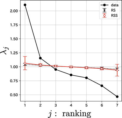
Figure 3 presents the scree graph for the eigenvalues where the abscissa represents the ranking, $j$, of each eigenvalue, while the ordinate indicates the magnitude of each eigenvalue ${\lambda }_j$.

Figure 3.

Distribution of eigenvalues.

The black line marked with filled circles corresponds to the distribution of eigenvalues obtained from the complex correlation matrix constructed from the data. The black dotted line marked with crosses and accompanied by error bars represents the distribution of the eigenvalues sourced from the complex correlation matrix generated using RS. The red line marked with open circles and error bars depicts the distribution of eigenvalues derived from the complex correlation matrix generated using RRS. We conducted 50 simulations for RS and RRS to determine their respective mean values and standard deviations. In this graph, the error bars represent three times the standard deviation.

By comparing these results, we confirm that the first eigenvalue is evidently the principal component, that is, $n_{\mathrm{p}}=1$.

4.2 Principal eigenvector

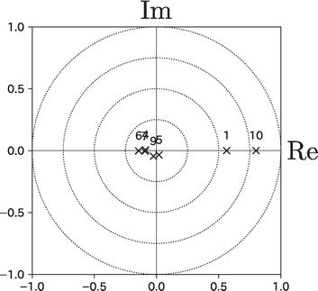
Figure 4 illustrates the distribution of the eigenvector that corresponds to the first eigenvalue. In this figure, the abscissa represents the real axis, while the ordinate represents the imaginary axis. Unlike the components in a real correlation matrix, the components of this eigenvector are distributed on a complex plane. To account for the nature of the eigenvectors in this figure, we imposed a constraint that sets the imaginary part of “10. Other Consumption Expenditures” to zero.

Figure 4.

Distribution of components of principal eigenvector.

In this context, two key quantities are the absolute value and the argument of each complex component. The absolute value signifies the strength of each component in the eigenvector. Therefore, “10. Other Consumption Expenditures” emerges as the most dominant factor, followed by “1. Food.”

The argument of the complex number indicates the leading and lagging relationships between the factors. As demonstrated in Eq. (10), each index rotates in a clockwise manner as time progresses. Nevertheless, Figure 4 reveals no typical leading or lagging relationships. Instead, the figure identifies three distinct groups: one consisting of “10. Other Consumption Expenditures” and “1. Food”; another comprising “4. Furniture & Household Utensils,” “6. Medical Care,” and “7. Transportation & Communication”; and a final group containing “5. Clothing & Footwear” and “9. Culture & Recreation.”

4.3 Mode signals

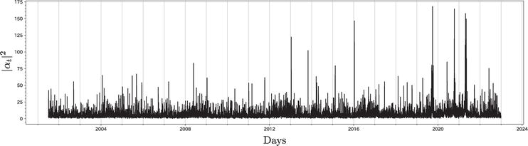
We consider the squared values of the mode signals defined by using the following expression:

$${\left|{\alpha }_t\right|}^2=\sum _{j\in J}{\left|{\alpha }_{j,t}\right|}^2,$$E19

where $J=\left\{\mathrm{1,4,5,6,7,9,10}\right\}$ represents the numbers corresponding to the various categories from the included in our analysis. We square the mode signals because their components consist of complex numbers. Figure 5 displays the mode signal as it is defined in Eq. (19).

Figure 5.

The sum of mode signals ${\left|{\alpha }_t\right|}^2$ for the Japanese family income and expenditure survey data.

In this figure, the abscissa represents the days, and the ordinate represents the squared values of the mode signals. Here, we focus on the peaks occurring after 2019. The top five peaks are summarized in Table 1, ordered according to time. The most significant peak occurred on September 30, 2019. This is the day before Japan’s consumption tax was increased from $8\%$ to $10\%$, October 1, 2019. The second peak falls on October 12, 2020, coinciding with the Japanese government’s “Go To Campaign” to stimulate the economy after the COVID-19 pandemic, which had decreased consumption. The third peak is observed on April 24, 2021, when Japan was in the midst of the fourth wave of its COVID-19 pandemic; a state of emergency was declared in four prefectures in the Tokyo metropolitan area on April 25, 2021. The fourth peak occurs on May 6, 2021 and corresponds to the declaration of a state of emergency for nine prefectures on May 12, 2021. Finally, the fifth peak occurs on April 18, 2021 and is attributed to the same factors as the third peak.

Data	Ranking of mode signal	Relating events
2019-09-30	1	Sales tax rate increases from 8–10% (October 1, 2019)
2020-10-12	2	Economic stimulus package for the COVID-19 pandemic
2021-04-18	5	State of emergency declared in four prefectures
2021-04-24	3	State of emergency declared in four prefectures (April 25, 2021)
2021-05-06	4	State of emergency declared in nine prefectures (May 12, 2021)

Table 1.

Five peaks of the sum of mode signals ${\left|{\alpha }_t\right|}^2$ after 2019 and the occurrence of related events.

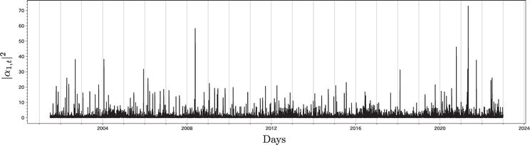
Next, we focus on the first mode signal ${\left|{\alpha }_{1,t}\right|}^2$. Figure 6 displays the mode signal of ${\left|{\alpha }_{1,t}\right|}^2$. In this figure, the abscissa represents the days, and the ordinate represents ${\left|{\alpha }_{1,t}\right|}^2$. Here, we once again focus on the peaks occurring after 2019. The top five peaks are summarized in Table 2, Unlike the data in Table 1, the most prominent peak for this mode signal is May 6, 2021 when Japan was in the midst of the fourth wave of its COVID-19 pandemic: A state of emergency had been declared for four prefectures in the Tokyo metropolitan area on April 25, 2021 and was extended to nine prefectures on May 12, 2021. The second peak falls on October 12, 2020, coinciding with the Japanese government’s “Go To Campaign” aimed at stimulating the economy due to the decline in consumption precipitated by the pandemic. The third peak is observed on April 26, 2021, 1 day after a state of emergency was declared for four prefectures in the Tokyo metropolitan area on April 25, 2021. The fourth peak occurs on September 24, 2021, a date not exhibited in Table 1, corresponding to the lifting of all emergency declarations on September 30, 2021. It should be noted that people had more opportunities to go out around this time, leading to increased consumption. Finally, the fifth peak occurs on September 30, 2019, the day before Japan’s consumption tax was increased from 8–10%, October 1, 2019, as explained in Table 1.

Figure 6.

The first mode signal ${\left|{\alpha }_{1,t}\right|}^2$ for the Japanese family income and expenditure survey data.

Data	Ranking of mode signal	Relating events
2019-09-30	5	Sales tax rate increases from 8–10% (October 1, 2019)
2020-10-12	2	Economic stimulus package for the COVID-19 pandemic
2021-04-26	3	State of emergency declared in four prefectures (April 25, 2021)
2021-05-06	1	State of emergency declared in nine prefectures (May 12, 2021)
2021-09-24	4	All emergency declarations lifted (September 30, 2021)

Table 2.

Five peaks of the first mode signal ${\left|{\alpha }_{1,t}\right|}^2$ after 2019 and relating events.

5. Conclusion

This chapter reviewed the methodology of CHPCA and examined the top 10 categories from the Japanese FIES for the January 1, 2000–June 30, 2023 period as a practical example, specifically delving into the periods preceding and following the COVID-19 pandemic. We identified characteristic days based on mode signal peaks and explored their relationship to the events occurring before and after the pandemic.

The most prominent peak in the sum of mode signals occurred on September 30, 2019, and the day before Japan’s consumption tax was increased from 8–10%, October 1, 2019. Other peaks were associated with the spread of COVID-19 and government stimulus measures. Interestingly, the mode signal for the principal component, which accounted predominantly for the spread of COVID-19 and government interventions during the pandemic, ranked fifth, following the peak associated with the tax increase.

The Japanese government initiated a special fixed benefit of 100,000 yen for all citizens in June 2020 as part of the economic stimulus measures implemented during the COVID-19 pandemic. This benefit was claimed by 99% of the population by September 2020. However, this paper’s CHPCA analysis did not detect that this measure had any significant impact. One explanation for this fact could be that the fixed benefit was spent gradually over several months and therefore did not cause an immediate spike in consumption. Another possibility is that the effect of the fixed benefit was too subtle to be captured by the FIES household survey.

Acknowledgments

I would like to thank Prof. H. Aoyama, Prof. Y. Fujiwara, Prof. H. Iyetomi, and Prof. H. Yoshikawa for useful discussions. This research was supported by a grant-in-aid for scientific research (KAKENHI), JSPS Grant Number 22 K04590.

References

1.Connor G, Korajczyk RA. Performance measurement with the arbitrage pricing theory: A new framework for analysis. Journal of Financial Economics. 1986;15(3):373-394
2.Ilmanen A. Time-varying expected returns in international bond markets. Journal of Finance. 1995;50(2):481-506
3.Stock JH, Watson MW. Forecasting using principal components from a large number of predictors. Journal of the American Statistical Association. 2002;97(460):1167-1179
4.Stock JH, Watson MW. Macroeconomic forecasting using diffusion indexes. Journal of Business & Economic Statistics. 2002;20(2):147-162
5.Bai J, Ng S. Determining the number of factors in approximate factor models. Econometrica. 2002;70(1):191-221
6.Kose MA, Otrok C, Whiteman CH. International business cycles: World, region, and country-specific factors. The American Economic Review. 2003;93(4):1216-1239
7.Bernanke BS, Boivin J, Eliasz P. Measuring the effects of monetary policy: A factor-augmented vector autoregressive (FAVAR) approach. The Quarterly Journal of Economics. 2005;120(1):387-422
8.Cattell RB. The screen test for the number of factors. Multivariate Behavioral Research. 1966;1(2):245-276
9.Marčenko VA, Pastur LA. Distribution of eigenvalues for some sets of random matrices. Mathematics of the USSR-Sbornik. 1967;1(4):457-483
10.Porter CE, Thomas RG. Fluctuations of nuclear reaction widths. Physical Review. 1956;104(2):483-491
11.Laloux L, Cizeau P, Bouchaud JP, Potters M. Noise dressing of financial correlation matrices. Physical Review Letters. 1999;83(7):1467-1470
12.Plerou V, Gopikrishnan P, Rosenow B, Amaral LAN, Stanley HE. Universal and nonuniversal properties of cross correlations in financial time series. Physical Review Letters. 1999;83(7):1471-1474
13.Plerou V, Gopikrishnan P, Rosenow B, Amaral LAN, Guhr T, Stanley HE. Random matrix approach to cross correlations in financial data. Physical Review E. 2002;65(6):066126
14.Utsugi A, Ino K, Oshikawa M. Random matrix theory analysis of cross correlations in financial markets. Physical Review E. 2004;70(2):026110
15.Kim DH, Jeong H. Systematic analysis of group identification in stock markets. Physical Review E. 2005;72(4):046133
16.Pan RK, Sinha S. Collective behavior of stock price movements in an emerging market. Physical Review E. 2007;76(4):046116
17.Namaki A, Shirazi AH, Raei R, Jafari GR. Network analysis of a financial market based on genuine correlation and threshold method. Physica A: Statistical Mechanics and its Applications. 2011;390(21–22):3835-3841
18.Namaki A, Jafari GR, Raei R. Comparing the structure of an emerging market with a mature one under global perturbation. Physica A: Statistical Mechanics and its Applications. 2011;390(17):3020-3025
19.Jamali T, Jafari GR. Spectra of empirical autocorrelation matrices: A random-matrix-theory–inspired perspective. EPL. 2015;111(1):10001
20.Markowitz H. Portfolio selection. The Journal of Finance. 1952;7(1):77-91
21.Fujiwara Y, Souma W, Murasato H, Yoon H. Application of PCA and random matrix theory to passive fund management. In: Takayasu H, editor. Practical Fruits of Econophysics. Tokyo: Springer; 2006. pp. 226-230
22.Souma W. Toward a practical application of Econophysics: An approach from random matrix theory (written in Japanese). Applied Mathematics. 2005;15(3):45-59
23.Lo AW, MacKinlay AC. An econometric analysis of nonsynchronous trading. Journal of Econometrics. 1990;45(1–2):181-211
24.Iyetomi H, Nakayama Y, Aoyama H, Fujiwara Y, Ikeda Y, Souma W. Fluctuation-dissipation theory of input-output interindustrial relations. Physical Review E. 2011;83(1):016103
25.Iyetomi H, Nakayama Y, Yoshikawa H, Aoyama H, Fujiwara Y, Ikeda Y, et al. What causes business cycles? Analysis of the Japanese industrial production data. Journal of the Japanese and International Economies. 2011;25(3):246-272
26.Arai Y, Yoshikawa T, Iyetomi H. Complex principal component analysis of dynamic correlations in financial markets. Frontiers in Artificial Intelligence and Applications. 2013;255:111-119
27.Arai Y, Yoshikawa T, Iyetomi H. Dynamic stock correlation network. Procedia Computer Science. 2015;60:1826-1835
28.Souma W. Characteristics of principal components in stock price correlation. Frontiers in Physics. 2021;9:602944
29.Vodenska I, Aoyama H, Fujiwara Y, Iyetomi H, Arai Y. Interdependencies and causalities in coupled financial networks. PLoS One. 2016;11(3):e0150994
30.Souma W, Aoyama H, Iyetomi H, Fujiwara Y, Irena V. Construction and application of new analytical methods for stock correlations: Toward the construction of prediction model of the financial crisis (written in Japanese). In: Proceeding of Network Emergent Intelligence Workshop. Tokyo: Japan Society for Software Science and Technology; 2016. pp. 1-8. Available from: http://www.ics.lab.uec.ac.jp/sig-ein/index.php?JWEIN2016
31.Souma W, Iyetomi H, Yoshikawa H. Application of complex Hilbert principal component analysis to financial data. In: IEEE 41st Annual Computer Software and Applications Conference (COMPSAC). Vol. 2. IEEE; 2017. pp. 391-394
32.Souma W, Iyetomi H, Yoshikawa H. The Leading and Lagging Structure of Early Warning Indicators for Detecting Financial Crises (Written in Japanese). RIETI Policy Discussion Paper Series; 18-P-005. Tokyo; 2018. pp. 1-26. Available from: https://www.rieti.go.jp/jp/publications/summary/18030017.html
33.Kichikawa Y, Iyetomi H, Iino T, Inoue H. Hierarchical and circulating flow structure in an interfirm transaction network. In: Abstracts of the 6th International Workshop on Complex Networks and their Applications; Lyon, France. 2017. pp. 12-14
34.Iyetomi H, Ikeda Y, Mizuno T, Ohnishi T, Watanabe T. International trade relationship from a multilateral. In: Abstracts of the 6th International Workshop on Complex Networks and their Applications; Lyon, France. 2017. pp. 253-255
35.Kichikawa Y, Iyetomi H, Iino T, Inoue H. Community structure based on circular flow in a large-scale transaction network. Applied Network Science. 2019;4(1):92. DOI: 10.1007/s41109-019-0202-8
36.Iyetomi H. Collective phenomena in economic system. In: Complexity, Heterogeneity, and the Methods of Statistical Physics in Economics. Singapore: Springer; 2020. pp. 177-201
37.Iyetomi H, Aoyama H, Fujiwara Y, Souma W, Vodenska I, Yoshikawa H. Relationship between macroeconomic indicators and economic cycles in US. Scientific Reports. 2020;10(1):1-12
38.Souma W, Roma CM, Goto H, Iyetomi H, Vodenska I. Complex Global Interdependencies between Economic Policy Uncertainty and Geopolitical Risks Indices. RIETI Discussion Paper Series; 22-E-028. Tokyo; 2022. pp. 1-36. Available from: https://www.rieti.go.jp/en/publications/summary/22030031.html
39.Statistics Bureau of Japan: Available from: https://www.stat.go.jp/english/data/kakei/index.html.
40.Statistical tables (in Japanese): Available from: https://www.e-stat.go.jp/stat-search/files?page=1&layout=datalist&toukei=00200561&tstat=000000330001&cycle=1&tclass1=000000330001&tclass2=000000330004&tclass3=000000330005&tclass4val=0.
Written By
Wataru Souma
Submitted: 31 August 2023Reviewed: 04 September 2023Published: 07 November 2023
Open access peer-reviewed chapter