Open Access is an initiative that aims to make scientific research freely available to all. To date our community has made over 100 million downloads. It’s based on principles of collaboration, unobstructed discovery, and, most importantly, scientific progression. As PhD students, we found it difficult to access the research we needed, so we decided to create a new Open Access publisher that levels the playing field for scientists across the world. How? By making research easy to access, and puts the academic needs of the researchers before the business interests of publishers.
We are a community of more than 103,000 authors and editors from 3,291 institutions spanning 160 countries, including Nobel Prize winners and some of the world’s most-cited researchers. Publishing on IntechOpen allows authors to earn citations and find new collaborators, meaning more people see your work not only from your own field of study, but from other related fields too.
To purchase hard copies of this book, please contact the representative in India:
CBS Publishers & Distributors Pvt. Ltd.
www.cbspd.com
|
customercare@cbspd.com
On March 11, 2011, the Great East Japan Earthquake struck the Tohoku Region of Japan. A huge area along the northeast coast of Japan was seriously damaged by earthquake with a magnitude of 9.0 and subsequent tsunami. The view of the coastline of the Tohoku Region was dramatically changed by the tsunami. Since then, the author and his group at Tokai University have been monitoring the recovery of the tsunami-damaged areas of Miyagi Prefecture through ground survey and satellite image data analysis. In this study, the authors have investigated how the NDVI seasonal variability of inundated paddy fields changed from year to year after the tsunami. The authors have selected two areas in Miyagi Prefecture in Japan for the test sites of the investigation. One is the paddy fields along the Kitakami River, and the other is the paddy fields in the Sennan Plain of Miyagi Prefecture. Usually, the NDVI of typical paddy fields in Miyagi Prefecture gradually increases from May to August and suddenly decreases in September due to harvesting. The NDVI trend analysis of both areas clarified how the location of paddy fields influenced recovery from the damages of the tsunami.
Tokai University, Research & Information Center, 2-3-23, Takanawa, Minato-ku, Tokyo
*Address all correspondence to: kohei.cho@tokai-u.jp
1. Introduction
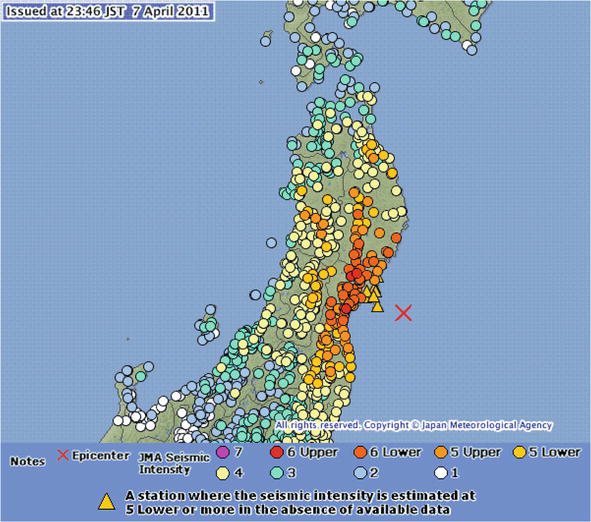
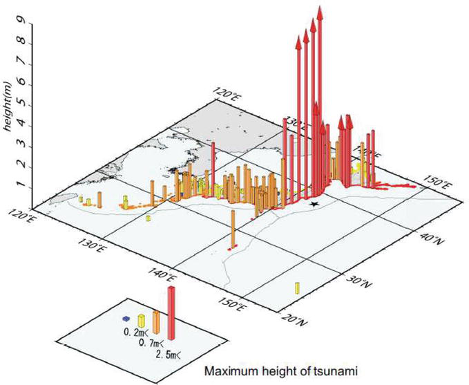
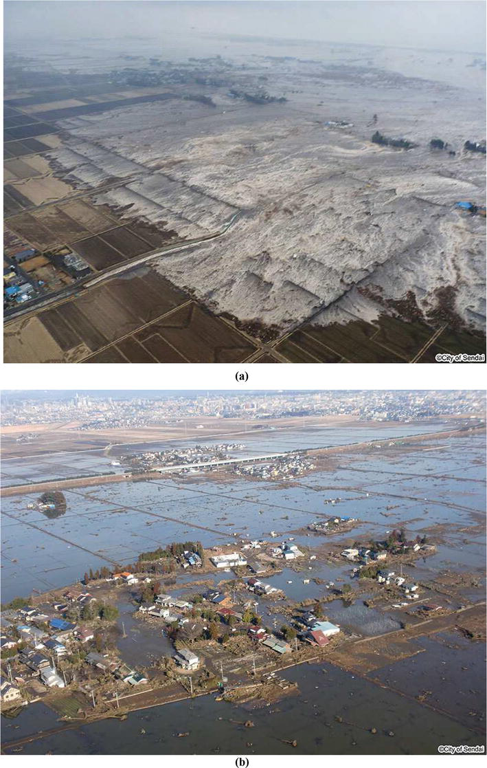
On March 11, 2011, the Great East Japan Earthquake with a magnitude of 9.0 struck the Tohoku Region of Japan. A huge area along the coast of the northeast coast of Japan was seriously damaged by the earthquake and subsequent tsunami. Figure 1 shows the epicenter and the seismic intensity distribution of the earthquake [1]. The maximum height of the tsunami was 9.3 m recorded in Soma, Fukushima Prefecture (see Figure 2). A total of 561 sq. km was inundated by the tsunami [2]. More than 19,000 people were lost and more than 2592 people are still missing [3]. The Great East Japan Earthquake can be characterized by the heavy damages caused by the huge tsunami. Figure 3 shows aerial photos of the paddy fields of Wakabayashi-ku, Sendai City, Miyagi Prefecture reflecting how seriously the area was damaged by the tsunami [4].
Figure 1.
Epicenter and seismic intensity distribution of the Japan Earthquake (Mar. 11, 2011, JMA) [1].
Figure 2.
Observed maximum height of tsunami (Mar. 11, 2011, JMA) [1].
Figure 3.
Aerial photos of Wakabayashi-ku, Sendai City, Miyagi Prefecture (provided by Sendai City). (a) Tsunami striking paddy fields (March 11, 2011) and (b) inundated paddy fields (March 14, 2011) [4].
More than 5000 satellite images were taken within 2 weeks after the disaster under international cooperation [5, 6, 7]. The comparison of the satellite images taken before and after the disaster enhanced the serious damages in the area. After the Great East Japan Earthquake, various studies on monitoring the damages of the earthquake and associated tsunami were performed. JAXA has taken a total of 643 images of the damaged areas using AVNIR2 and PALSAR onboard the ALOS satellite, and these images were used for damage analysis [8]. Koshimura et al. [9] reviewed how remote sensing methods have been used to contribute to post-tsunami disaster response. Remote sensing is a necessary technology for monitoring the damages of disasters. Liou et al. [10] analyzed MODIS data of before (2010) and after (2011) the tsunami, and evaluated the area of rice fields lost by the tsunami. They estimated the total loss area of paddy fields after the tsunami using MODIS data. However, remote sensing should also be used for monitoring the recovery of the damaged areas. Since 2011, the authors are monitoring the recovery of the tsunami-damaged areas of the Miyagi Prefecture by ground survey and satellite image data analysis [11, 12, 13, 14]. In this study, the author and his team have applied a multitemporal analysis of MODIS NDVI to evaluate the recovery status of paddy fields [15].
The authors have selected two areas in Miyagi Prefecture in Japan as the test sites for the investigation. One is the paddy fields along the Kitakami River, and the other is the paddy fields in the Sennan Plain.
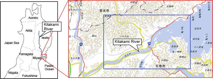
2.1 Kitakami River
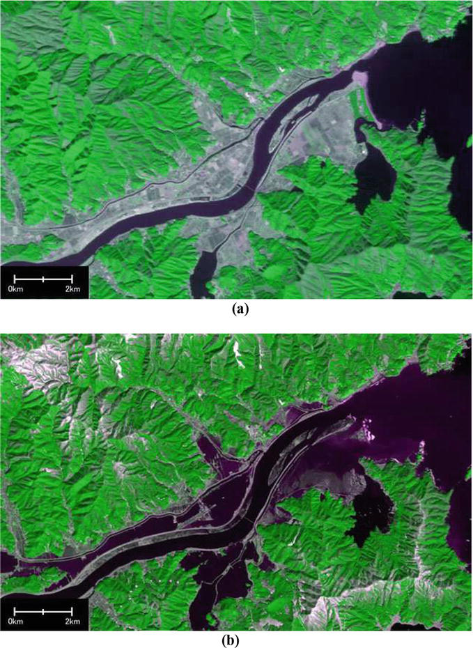
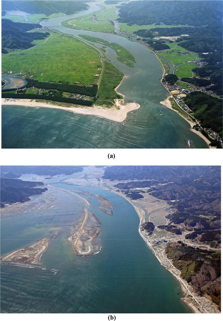
The Kitakami River is the fourth largest river in Japan with a length of 249 km. The source of the river is in the northern part of Iwate Prefecture and it flows down to Miyagi Prefecture. In Miyagi Prefecture, the river bends to the east and flows into the Pacific Ocean (see Figure 4). Figure 5 shows the optical sensor AVNIR2 images taken from the ALOS satellite of JAXA before and after the tsunami. It is clear that a huge area of paddy fields along the river was inundated by the tsunami. Figure 6 shows the aerial photos of the mouth of the river taken before and after the tsunami. It is shocking to see how the scenery of the mouth of the river is completely changed by the tsunami.
Figure 4.
Map of the Kitakami River before the tsunami (blue square frame corresponds to the area of Figure 5). (Source: GSI Maps).
Figure 5.
ALOS/AVNIR2 images of the Kitakami River taken before and after the tsunami (AVNIR2: Band 1: Blue, Band 3: Red, Band 4: Green, provided by JAXA). (a) February 27, 2011 and (b) March 19, 2011.
Figure 6.
Aerial photos of the mouth of Kitakami River taken before and after the Tsunami [16]. (a) July, 1995 and (b) April 4, 2011.
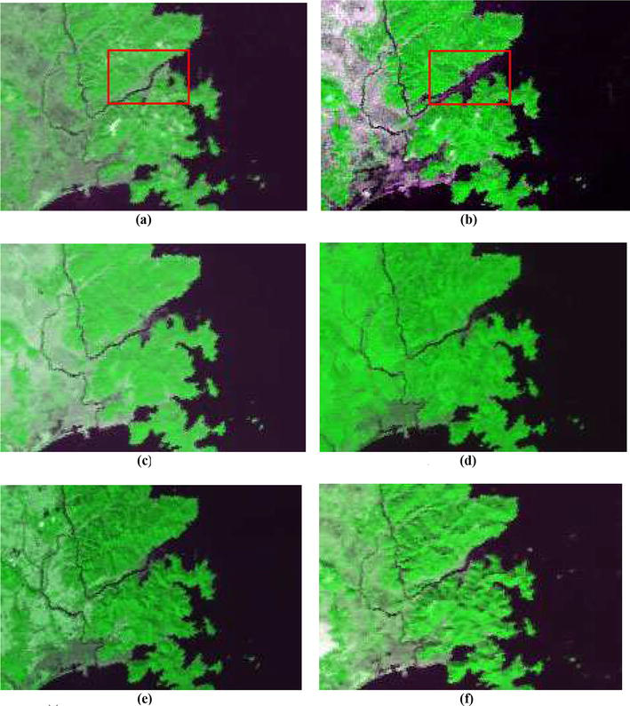
Figure 7 shows MODIS false composite images around the Kitakami River. By looking at the time series of MODIS images, we can recognize the changes in the form of the river reflecting the damage and recovery along the river. However, on the other hand, it is also clear that the 250-m special resolution of MODIS is not enough for spatially evaluating the damages and recovery of the paddy fields in this area. As a result, considering that MODIS can observe the same area every day, the author has decided to monitor the damages and recovery by comparing the time series of MODIS NDVI of particular paddy fields.
Figure 7.
Time series of MODIS images of Kitakami River and it’s surroundings. The red rectangle corresponds to the area of Figure 4 (MODIS Band 1: blue, red, Band 2: Green). (a) February 16, 2011, (b) March 13, 2011, (c) April 5, 2011, (d) August 13, 2011, (e) October 19, 2011 and (f) December 24, 2011.
2.2 Sennan Plain
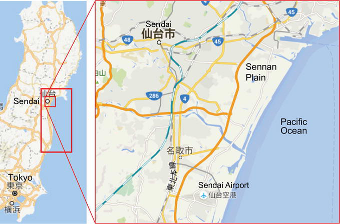
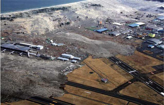
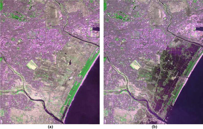
The second test site we selected is Sennan Plain of Miyagi Prefecture. The Sennan Plain is located in the southeast along the coast of Miyagi Prefecture facing the Pacific Ocean as shown in Figure 8. Huge agricultural fields, mostly paddy fields, of the Sennan Plain were seriously inundated by the tsunami. Figure 9 shows an aerial photo of Sendai Airport that was taken at the time when the tsunami inundated the area on March 11, 2011, after the earthquake. Figure 10 shows the AVNIR2 images of this area taken before and after the tsunami. It is obvious that most of the paddy fields along the coast were inundated by the tsunami. The dotted line box in Figure 8 shows the test site for evaluating how the 16 days of MODIS images were composed into a single image (see Chapter 3).
Figure 8.
Location of the test site. (Source: Google Maps).
Figure 9.
Aerial photo of the Sendai Airport and it’s surroundings (March 11, 2011 Japan Coast Guard).
Figure 10.
ALOS/AVNIR2 images of the Wakabayashi-ku taken before and after the Tsunami (AVNIR2: Band 1: blue, Band 3: red, Band 4: green, provided by JAXA). (a) February 27, 2010 and (b) March 14, 2011.
NDVI (Normalized Difference Vegetation Index) defined by the following formula is a typical index for estimating the condition of vegetation [17].
NDVI=NIR–VIS/NIR+VISE1
Where NIR: near infrared band; VIS: visible red band.
Since inundated paddy fields are likely to reduce the reflectance of NIR, the damages may be enhanced in the value reduction of NDVI. In this study, NDVI derived from MODIS data of the Terra satellite was used for the analysis. Table 1 shows the specifications of MODIS. For calculating NDVI with formula (1), MODIS Band 1 is used for VIS, and Band 2 is used for NIR. As for the test site of the Kitakami River, MODIS NDVI monthly composite data provided by GSI (Geospatial Information Authority of Japan) was used [19]. As for the test site of the Sennan Plain, the 16-day composite of MODIS NDVI dataset (MOD13Q1 [18, 20, 21]) provided by NASA [23] was analyzed. AVNIR2 images of the ALOS satellite of JAXA were used as the reference for selecting the sample areas. Table 2 shows the specification of AVNIR2 [24].
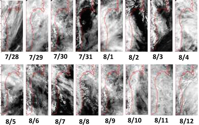
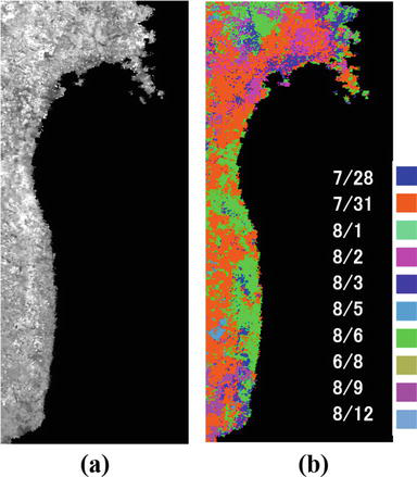
Figure 11 shows 16 MODIS Band 1 images of the area of the dotted line box in Figure 8 from July 28 to August 12, 2014. Certain areas of each image are covered with clouds. Table 3 shows the pixel reliability key [22] of MODIS provided by NASA. This pixel reliability data is used in MOD13Q1 when calculating 16-day composite MODIS NDVI. In addition, Band 3 was used for detecting the bright area such as clouds or snow. For example, if only the data of three days among 16 days were Good Data (0) and the others were No Data (−1), the three days data are averaged for calculating the 16-day composite. Figure 12(a) shows the result of 16-day composite. Most of the clouds are well rejected. Figure 12(b) shows which day was used for each location. This image shows that though the image was acquired within 16 days, the exact observation dates of NDVI are quite different from pixel to pixel.
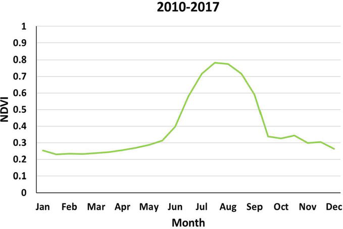
Figure 13 shows the typical MODIS NDVI seasonal variability of normal paddy fields in Miyagi Prefecture. This graph was derived by averaging monthly NDVI of normal paddy fields that were not suffered by the Tsunami from 2010 to 2017. In Tohoku Region, the NDVI of a paddy field gradually increases from May after the rice planting and reaches to a peak in August. From September to October, NDVI suddenly goes down after the harvesting. The author has examined how this seasonal NDVI pattern changed before and after the Tsunami.
Figure 13.
MODIS NDVI seasonal variability of normal paddy field. (Monthly NDVI data were averaged from 2010 to 2017).
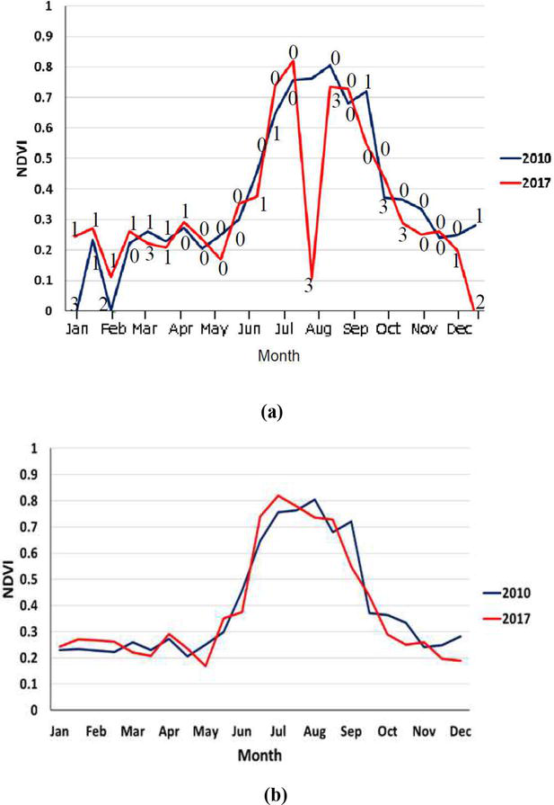
4.2 Interpolation of irregular value of NDVI in the 16-day composite
When we checked the NDVI seasonal variation of various paddy fields using the 16-day composite of MODIS NDVI, irregular reductions in NDVI value were often observed. Figure 14 shows such an example. The graph for 2017 has an abnormal reduction of NDVI in July. The graph of 2010 also has reductions in January and February. The numbers in the graph correspond to the pixel reliability key described in Table 3. “2” corresponds to snow/ice and “3” corresponds to clouds. So, we can understand that a big reduction of NDVI values was caused by the snow or clouds cover during 16 days. These irregular values of NDVI make it difficult to understand the condition of the paddy fields. On the other hand, even though the pixel reliability key is “3” (cloudy), many of the NDVI values looked normal. So, simply using the pixel reliability key for extracting irregular values is not appropriate. Also, it has become clear that most of the points where the NDVI was 0 were the areas that were covered with snow. These problems had to be solved. The authors have examined ways to extract the irregular value of NDVI by comparing the NDVI value before and after the period. In this study, we defined the following two equations to interpolate the irregular value of NDVI.
Figure 14.
MODIS NDVI seasonal variability of normal paddy field. (a) Original NDVI and (b) interpolated NDVI.
If NDVI(t − 1) − NDVI(t) > 0.1 and
If NDVI(t + 1) − NDVI(t) > 0.1
or NDVI(t) = 0
then
NDVIt=NDVIt−1+NDVIt+1/2E2
If NDVI(t)<0.1 and If NDVI(t + 1) <0.1
then
NDVIt=NDVIt−1+NDVIt+2/2E3
t: target period (1 to 23).
The result of applying this method is shown in Figure 14(b). The seasonal variability became similar to the normal paddy field shown in Figure 13.
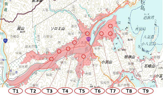
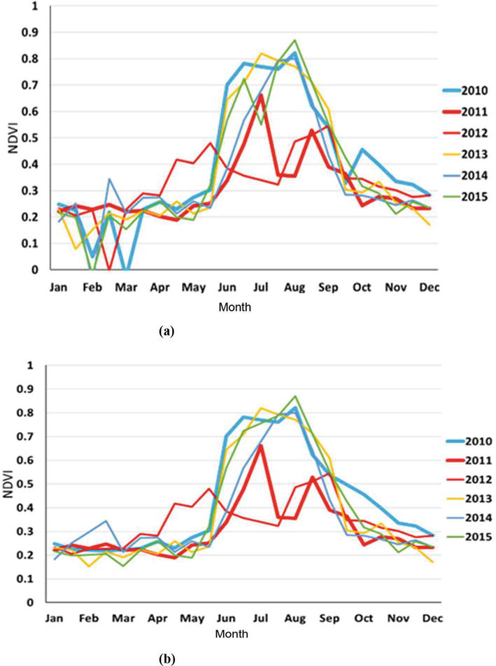
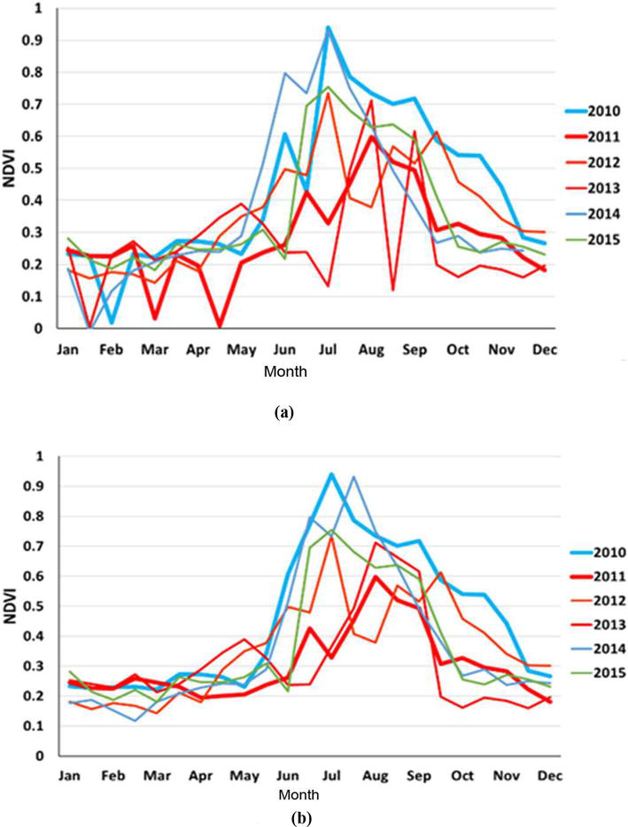
As shown in Figures 5 and 6, the Kitakami River was seriously damaged by the Tsunami. In order to evaluate the damage difference of the paddy fields located along the Kitakami River, the author have selected nine sample points, namely T1 to T9, as shown in Figure 15. The map is an inundated map produced by GSI after the Tsunami. The pink areas correspond to the inundated areas. Figure 16 shows the seasonal NDVI variability graph of 2009 to 2012 for each sample point.
Figure 15.
Sample point of NDVI plotted on the inundated map of the Kitakami River.
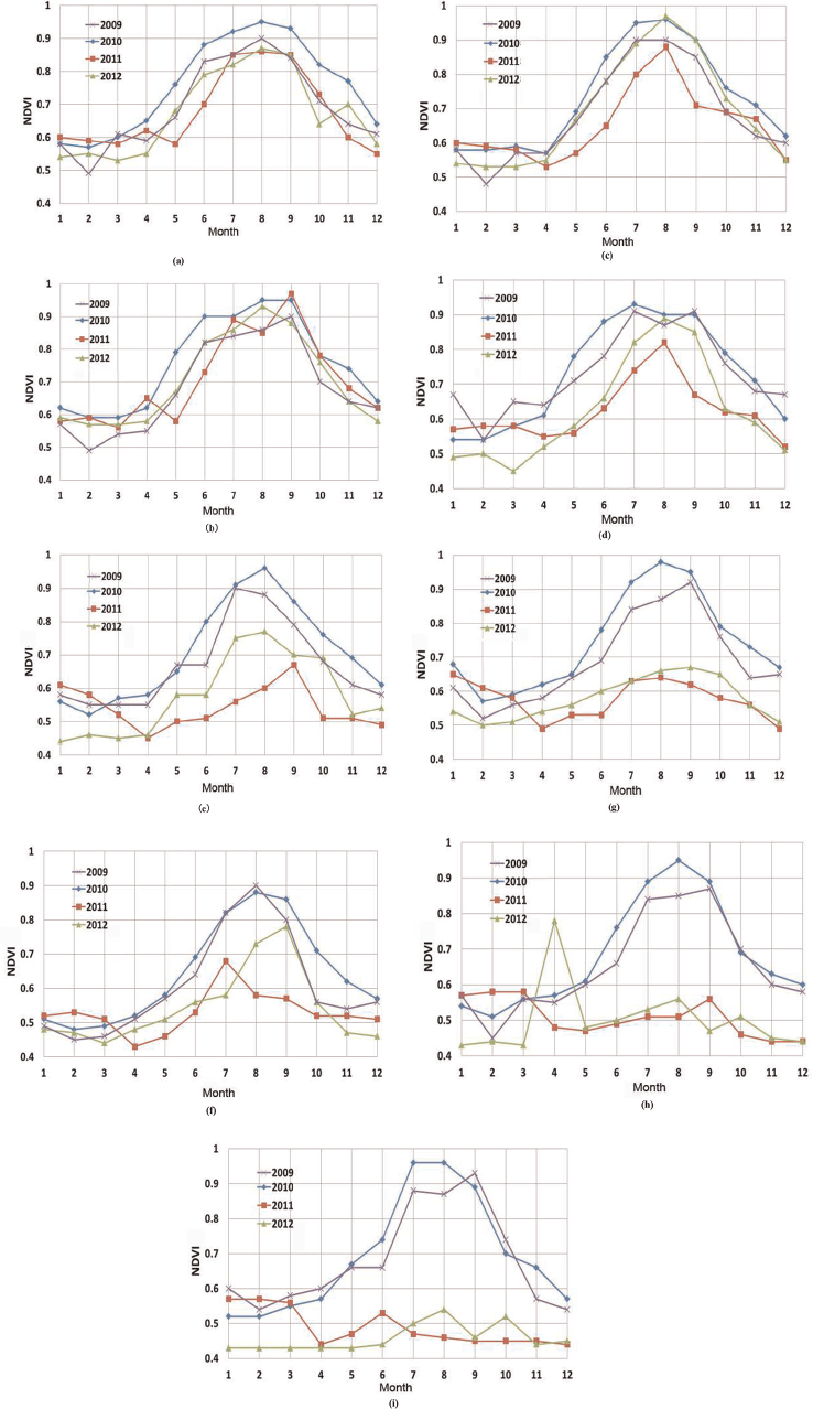
Figure 16.
Seasonal NDVI Variability comparison of the nine sample points. (a) T1, (b) T2, (c) T3, (d) T4, (e) T5, (f) T6, (g) T7, (h) T8 and (i) T9.
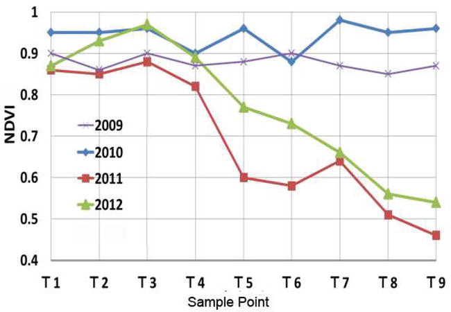
We compare seasonal NDVI graphs shown in Figure 16, all the graph patterns of 2009 and 2010, before the tsunami looks similar to the pattern of the normal paddy fields as shown in Figure 13. However, the patterns of 2011 and 2012 are quite different from one sample point to the other. Particularly, if we compare the patterns of the year 2011, it is clear that the NDVI values gradually reduced from T1 to T9. These changes can be explained as follows. The damages of the paddy fields far from the river mouth, namely sample points T1 to T4, were not much. The damages of the paddy fields in the middle, namely sample points T5 and T7, were quite serious. Finally, the damages of the paddy fields near in the mouth of the river, namely sample points T8 and T9, were most serious, and NDVI value did not go up to more than 0.6 throughout the years of 2011 and 2012.
Figure 17 shows the NDVI comparison of August from T1 to T9 for 2009 to 2012. The NDVI values of T1 to T9 are almost the same for 2009 and 2010. However, as for 2011, the NDVI value dramatically reduced from T1 to T9 reflecting the damage difference of paddy fields according to the distance from the mouth of the river. Though the pattern of 2012 is similar to the pattern of 2011, some increase of NDVI value can be observed reflecting the recovery of the paddy field. The paddy fields around the mouth of the river were completely destroyed and needed to be reclaimed to reconstruct the paddy fields, and the author terminated the NDVI comparison of the paddy fields around the Kitakami River and shifted to the detailed study of the paddy fields in the Sennan Plain.
Figure 17.
NDVI comparison of August from 2009 to 2012 of the sample points T1 to T9.
5.2 Sennan Plain
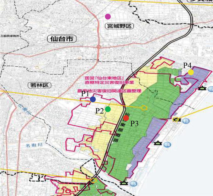
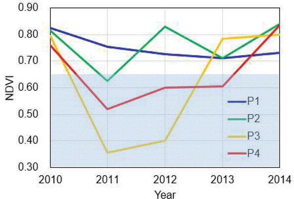
Figure 18 shows a part of the agricultural recovery map of the Sendai Area prepared by the Miyagi Prefectural Government [25]. The area framed in red is the area that suffered from the Tsunami. The area colored in white corresponds to the area where the tsunami did not come or was not much affected by the tsunami. The area colored in yellow corresponds to the area where the recovery project started in 2011, the green area started in 2012, and the purple area started in 2013. It is quite reasonable that the agricultural recovery project started from the inland areas where the damages of the tsunami were lighter than the inshore areas. Then, the recovery project was expanded toward the inshore areas. To evaluate the status of the recovery project, the authors have selected four sample points as shown in Figure 18.
shows the sample point P1 selected from the normal inland paddy field that was not affected by the tsunami.
shows the sample point P2 selected in the area of recovery project started in 2011.
shows the sample point P3 selected in the area of recovery project started in 2012, and
shows the sample point P4 selected in the area of recovery project started in 2013.
Figure 18.
Paddy Field Recovery Project Map [24].
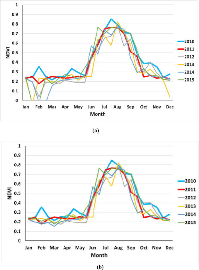
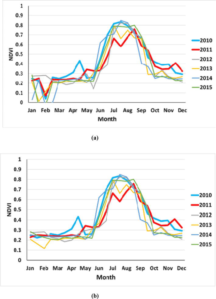
The interpolation method was applied to the 16-day composite MODIS NDVI for the paddy fields selected in Figure 18. The result of before and after applying the method to the MODIS NDVI seasonal variabilities from 2010 to 2015 is shown in Figures 19–22. In all four figures, by applying the proposed interpolation method, irregular reduction of NDVI during the winter due to the snow cover (see (a) of each figure) was well interpolated by the data of before and after the period, and the normal paddy filed pattern became clear in (b) of each figure. At the same time, the NDVI reduction patterns in the year 2011 and afterward due to the effects of the tsunami were well preserved after applying the interpolation method.
Figure 19.
MODIS NDVI seasonal variability of a normal paddy field (sample point P1). (a) Before interpolation and (b) after interpolation.
Figure 20.
MODIS NDVI seasonal variability of inundated inland paddy field (sample point P2). (a) Before interpolation and (b) after interpolation.
Figure 21.
MODIS NDVI seasonal variability of inundated inshore paddy field (sample point P3). (a) Before interpolation and (b) after interpolation.
Figure 22.
MODIS NDVI seasonal variability of seriously inundated inshore paddy field (sample point P4). (a) Before interpolation and (b) after interpolation.
The NDVI values from July to August were averaged and plotted from 2010 to 2014 for the four sample points as shown in Figure 23. If we assume that the paddy fields whose NDVI values were less than 0.65 were damaged by the tsunami, we may conclude as follows. The NDVI values of sample point P1, the normal paddy field, are all over 0.7 reflecting the no damage from the tsunami. As for sample point P2, the inundated paddy field where the recovery project started in 2011 reduced the NDVI value from 0.83 to 0.63 in 2011, but recovered to 0.83 in 2012. As for sample point P3, the inundated inshore paddy field where the recovery project started in 2012 reduced the NDVI value from 0.79 to 0.35 in 2011 and 0.4 in 2012, but recovered to 0.78 in 2013. As for sample point P4, the inundated inshore paddy field where the recovery project started in 2013 reduced the NDVI value from 0.76 to 0.53 in 2011, and 0.60 in 2012 and 2013, but recovered to 0.83 in 2014. The result suggests that the recovery project was performed steadily, and the recovery of the paddy fields was achieved within a year in each project.
Figure 23.
MODIS NDVI variability of the four sample points for each summer.
In this study, the authors have investigated how the NDVI seasonal variability of paddy fields changes before and after the tsunami that struck the Tohoku Region of Japan on March 11, 2011. The authors have selected two areas, namely the paddy fields along the Kitakami River and in the Sennan Plain of Miyagi Prefecture, as the test sites of this study.
As for the Kitakami River, the difference in the damages of the tsunami was clearly reflected in the seasonal variability of NDVI. The inundated paddy fields located on the upper side of the River shows similar NDVI seasonal variability with normal paddy field in 2011 and also in 2012. This means that the inundated paddy fields on the upper side of the river were not as serious as the lower side of the river. However, the NDVI seasonal variability pattern of the inundated paddy fields near the mouth of the river was quite different for 2011 and 2012. The result reflected the heavy damage to the paddy fields in this area.
Time series of the 16-day composite of MODIS NDVI data were analyzed for evaluating the recovery speed of paddy fields in the Sensan Plain. As a result, in the inland area where the agricultural recovery project started in 2011, the paddy fields recovered within 1 year. As for the paddy fields located between the inland and inshore, the agricultural recovery project started in 2012 and the paddy fields recovered in 2012. The agricultural recovery project started in 2012 for the paddy fields located at inshore, and the paddy fields were recovered in 2013. By looking only at the results, you may say that every damaged paddy field analyzed in this study recovered within 1 year after performing the agricultural recovery project. But, maybe this is not true. The local government may have investigated the damages of the inundated paddy fields and systematically scheduled the agricultural recovery project. As a result, not all, but most of the paddy fields in this region successfully recovered within 3 years.
As the conclusion of this study, we may say that the seasonal variability evaluation of MODIS NDVI is quite useful for monitoring the damage and recovery condition of paddy fields. However, the spatial resolution of MODIS is too low for applying the classification method to evaluate the recovery condition of the damaged paddy fields. The paddy field of this region is not so large to be identified with MODIS data, and the mixed pixel problem may reduce the accuracy of the result. A higher resolution optical sensor such as the Sentinel-2/MSI with a revisit cycle of fewer days may be needed for applying the classification method.
This study was performed under the framework of “Monitoring Environmental Recovery of Damaged Area in Tohoku, Japan from Space & Ground for Environmental Education” under the Grants-in-Aid for Scientific Research sponsorship by MEXT (Ministry of Education, Culture, Sports, Science and Technology) and JSPS (The Japan Society for the Promotion of Science). The financial support from the Remote Sensing Technology Center (RESTEC) was also very helpful. The author would like to thank them for their kind support. The author also would like to thank the students of his lab, namely Mr. Ryota Uemachi and Mr. Kota Yamamoto, who worked hard with me in the past. Their contribution was outstanding.
References
1.JMA. The 2011 Off the Pacific Coast of Tohoku Earthquake Observed Tsunami. 2011. Available from: http://www.jma.go.jp/jma/en/2011_Earthquake/chart/2011_Earthquake_Tsunami.pdf
2.Nagayama T, Inaba K, Hayashi T, Nakai H. How the National Mapping Organization of Japan responded to the Great East Japan Earthquake? Proceedings of FIG Working Week. 2012;2012(TS03K-5791):1-15
3.Fire and Disaster Management Agency (FDMA). 2016. Available from: http://www.fdma.go.jp/bn/higaihou/pdf/jishin/158.pdf
4.Sendai City. 2023. Available from: https://www.city.sendai.jp/shiminkoho/shise/daishinsai/zenkoku/photoarchive/engan/index.html
5.Takahashi M, Shimada M. 2012, Disaster monitoring by JAXA for Japan Earthquake using satellites. Journal of the Japan Society of Photogrammetry and Remote Sensing. 2011;50(4):198-205
6.International Charter. 2022. Available from: https://www.disasterscharter.org/
7.Sentinel Asia. 2022. Available from: https://sentinel-asia.org/index.html
8.JAXA. Report on JAXA’s Response to the Great East Japan Earthquake. 2012. Available from: https://earth.jaxa.jp/en/application/disaster/20110311report-e/index.html
9.Koshimura S, Moya L, Mas E, Bai Y. Tsunami damage detection with remote sensing: A review. Geosciences. 2020;10(5):177. DOI: 10.3390/geosciences10050177
10.Liou Y, Sha H, Chen T, Wang T, Li Y, Lai Y, et al. Assessment of disaster losses in rice field and yield after tsunami induced by the 2011 Great East Japan earthquake. Journal of Marine Science and Technology. 2012;20(6):618-623. DOI: 10.6119/JMST-012-0328-2
11.Cho K, Fukue K, Uchida O, Terada K, Chen CF. Monitoring environmental recovery of damaged area in Tohoku, Japan from Space & Ground for Environmental Education. In: Proceedings of the 34th Asian Conference on Remote Sensing, SC03. AARS. 2013. pp. 709-716
12.Cho K, Baltsavias E, Remondino F, Soergel U, Wakabayashi H. RAPIDMAP project for disaster monitoring. In: Proceedings of the 35th Asian Conference on Remote Sensing, OS-145. AARS. 2014. pp. 1-6
13.Cho K, Fukue K, Uchida O, Terada K, Wakabayashi H, Sato T, et al. A study on detecting disaster damaged areas. In: Proceedings of the 36th Asian Conference on Remote Sensing, SP.FR2. AARS. 2015. pp. 1-4
14.Cho K, Uchida O, Terada K, Wakabayashi H, Sato T. Monitoring the recovery of the Tsunami damaged areas using satellite observation and field survey for environmental education. In: Proceedings of the 43rd Asian Conference on Remote Sensing, ACRS22_106. AARS. 2022. pp. 1-10
15.Uemachi R, Naoki K, Cho K. Monitoring the recovery of tsunami damaged paddy fields using MODIS NDVI. In: Proceedings of the 38th Asian Conference on Remote Sensing, PS-04-ID-844. 2017. pp. 1-4
16.Kappa club. 2014. Available from: http://www.michinoku.ne.jp/~kappa/
17.Weier J., D. Herring, 2000. Available from: http://earthobservatory.nasa.gov/Features/MeasuringVegetation/
18.NASA. 2017. MODIS Specifications. Available from: https://modis.gsfc.nasa.gov/about/specifications.php
19.GSI. 2012. Available from: https://www.gsi.go.jp/kankyochiri/ndvi.html (In Japanese)
20.NASA. 2017. MODIS Specifications. Available from: https://modis.gsfc.nasa.gov/about/specifications.php
21.Huete A, Didan K, Miura T, Rodriguez EP, Gao X, Ferreira LG. Overview of the radiometric and biophysical performance of the MODIS vegetation indices. Remote Sensing of Environment. 2002;83:195-213
22.Solano R., K. Didan, A. Jacobson, A. Huete. MODIS Vegetation Index User’s Guide. 2012. Available from: https://vip.arizona.edu/documents/MODIS/MODIS_VI_UsersGuide_01_2012.pdf
23.NASA LAADS DAAC. 2023. Available from: https://ladsweb.modaps.eosdis.nasa.gov/search/
24.JAXA. AVNIR-2 Advanced Visible and Near Infrared Radiometer Type 2. 2018. Available from: https://www.eorc.jaxa.jp/ALOS/en/alos/sensor/avnir2_e.htm
25.Miyagi Prefectural Government. 2015. Available from: http://www.pref.miyagi.jp/site/touhoku-saigai/nn-pamphlet-h27.html
Written By
Kohei Cho
Submitted: 10 July 2023Reviewed: 11 July 2023Published: 18 August 2023
 Open access peer-reviewed chapter