Solar Power Prediction with Artificial Intelligence

Abstract

Solar power prediction is a critical aspect of optimizing renewable energy integration and ensuring efficient grid management. The chapter explore the application of artificial intelligence (AI) techniques for accurate solar power forecasting. The AI models considered include Artificial Neural Networks (ANN), Support Vector Machines (SVM), Random Forest, and Gradient Boosting. These models are selected based on their ability to capture complex patterns and non-linear relationships present in the solar energy data. The solar power forecasting process involves data preprocessing, feature selection, model training, and evaluation. Data preprocessing techniques are applied to handle missing values and normalize the data to improve model performance. Feature selection methods are utilized to identify the most relevant features that influence solar power generation. The AI models are trained using historical data, where they learn the relationships between input features and solar power generation. Model evaluation is carried out using metrics such as Mean Squared Error (MSE) and Root Mean Squared Error (RMSE) to assess the accuracy of the forecasts. Furthermore, the forecasted results are visualized through line plots and error plots to provide valuable insights to stakeholders. A comprehensive report detailing the forecasting process, methodology, and results is generated, allowing decision-makers to make informed choices based on the forecasted solar energy data.

1. Introduction

While solar energy presents numerous benefits, its integration into the electricity grid introduces challenges related to its inherent intermittency and variability. Unlike conventional power sources like coal or natural gas plants that can produce a consistent output, solar power production fluctuates based on weather conditions, time of day, and geographical location. These fluctuations make it challenging for grid operators to maintain grid stability and ensure a reliable power supply.

Solar power forecasting plays a crucial role in addressing the challenges posed by solar energy’s intermittent nature. Accurate solar power forecasts enable grid operators to anticipate fluctuations in solar generation and plan grid operations accordingly. By having precise forecasts of solar power production, utilities can optimize the use of solar energy while efficiently managing conventional power generation sources for backup.

Effective solar power forecasting contributes to grid stability and reduces the need for fossil fuel-based backup power generation. Integrating solar power forecasts into energy management systems allows for better coordination of electricity generation, distribution, and demand response strategies. It enables grid operators to optimize the dispatch of power resources, thus minimizing energy wastage and reducing overall operational costs.

The ability to predict solar power production aids in avoiding imbalances between forecasted and actual generation, which can lead to financial penalties or missed revenue opportunities.

Governments worldwide are increasingly setting renewable energy targets and implementing supportive policies to promote the adoption of solar power and other clean energy sources. Solar power forecasting is a critical component of these policies, as it helps grid operators meet renewable energy integration mandates and transition towards a low-carbon energy future.

In recent years, significant advancements in forecasting technology have improved the accuracy of solar power forecasts. Advanced weather modeling, artificial intelligence, machine learning algorithms, and high-resolution satellite imagery have enhanced the precision and lead times of solar power predictions.

In an era marked by the escalating demand for clean and sustainable energy sources, solar power has emerged as a promising solution to address the global energy challenge. As the world seeks to transition from fossil fuels to renewable resources, the efficient integration of solar energy into power systems assumes paramount importance. This necessitates the development of accurate solar power prediction models that enable optimal energy management and grid operation. The fusion of artificial intelligence (AI) techniques with solar power forecasting holds tremendous potential in realizing this objective.

This chapter delves into the realm of solar power prediction, focusing on the application of AI methodologies to enhance the accuracy and reliability of solar power forecasts. The underlying premise is that accurate predictions enable stakeholders to make informed decisions, thereby facilitating the seamless integration of solar energy into the broader energy landscape. By employing AI models, such as Artificial Neural Networks (ANN), Support Vector Machines (SVM), Random Forest, and Gradient Boosting, this chapter explores how intricate patterns and non-linear relationships inherent in solar energy data can be effectively captured.

Solar power forecasting, a multifaceted process, encompasses several stages aimed at transforming raw data into actionable insights. These stages include data preprocessing, feature selection, model training, evaluation, and visualization. Data preprocessing techniques are crucial to handle missing values and normalize data, thereby enhancing the performance of AI models. Feature selection methodologies contribute to identifying the most influential variables that impact solar power generation, streamlining the forecasting process.

The AI models employed in solar power prediction are trained using historical data, enabling them to discern intricate connections between input features and solar power output. The process involves extracting underlying trends and correlations, a task ideally suited to AI’s prowess in pattern recognition. Model evaluation is paramount to ascertain the accuracy of predictions. Metrics such as Mean Squared Error (MSE) and Root Mean Squared Error (RMSE) serve as benchmarks to gauge the fidelity of forecasts, ensuring that the developed models meet rigorous performance standards.

Visualizing the forecasted results adds an essential layer of comprehension for stakeholders. Line plots and error plots offer intuitive insights, facilitating a clear understanding of the forecast’s reliability and potential areas for improvement. The visualization component bridges the gap between technical complexity and practical applicability, empowering decision-makers to make informed choices based on the forecasted solar energy data.

Moreover, the culmination of these efforts is a comprehensive report, detailing the forecasting process, methodologies employed, and the resultant outcomes. This report empowers decision-makers and stakeholders with a comprehensive understanding of the forecast’s underpinnings, enabling them to navigate the intricacies of solar power integration with confidence.

In summary, the marriage of AI techniques with solar power prediction presents an unprecedented opportunity to optimize renewable energy integration and streamline grid management. The ensuing exploration will delve into the specific AI models employed, the intricacies of the forecasting process, and the tangible benefits that accurate solar power predictions offer to the energy landscape. By unveiling the synergy between artificial intelligence and solar energy, this chapter aims to catalyze advancements that are instrumental in shaping a sustainable and resilient future powered by the sun’s abundant rays.

The dynamic landscape of renewable energy has underscored the pivotal role of solar power forecasting in optimizing the integration of solar energy into the electricity grid. Accurate predictions of solar irradiance and energy production are fundamental to ensuring efficient grid management and harnessing the potential of solar power. Recent years have witnessed a surge in the development of diverse forecasting models and techniques, aimed at enhancing the precision of solar power predictions. This research chapter embarks on a comprehensive exploration, analysis, and evaluation of various solar power forecasting models, encompassing statistical, machine learning, and physical approaches. By scrutinizing the strengths and limitations of each method, this study aspires to contribute to the evolution of solar power forecasting technology, fostering the seamless integration of solar energy into mainstream energy systems.

2. Literature review for solar energy prediction

A wealth of research has contributed valuable insights to the realm of solar energy prediction. Studies have explored diverse avenues, from machine learning techniques to hybrid models and ensemble learning, each enhancing our ability to forecast solar power outputs.

Numerous previous studies have delved into the realm of solar energy prediction, exploring diverse methodologies to enhance the accuracy of forecasts. These investigations have shed light on the efficacy of various approaches and models, contributing to the evolution of solar power forecasting technology.

Application of Machine Learning Techniques, a study conducted by Smith et al. [1] investigated the application of machine learning techniques, including Random Forest and Support Vector Machines, for solar power prediction. Their findings revealed that these algorithms demonstrated improved predictive accuracy compared to traditional methods. The study highlighted the potential of machine learning to capture complex solar energy patterns and enhance forecasting precision.

Integration of Numerical Weather Prediction Models, incorporating numerical weather prediction models, a study by Garcia-Soriano et al. [2] showcased the benefits of coupling AI models with meteorological insights. Their hybrid approach, combining Artificial Neural Networks with numerical weather prediction data, yielded more robust solar power predictions. This integration enabled a more holistic understanding of solar energy dynamics and bolstered forecast accuracy.

Ensemble Learning for Enhanced Predictions, the study by Zhang et al. [3] explored the efficacy of ensemble learning techniques, such as Gradient Boosting and AdaBoost, in solar power forecasting. Their research demonstrated that ensemble models outperformed individual models by mitigating model biases and uncertainties. The findings underscored the potential of ensemble learning to yield more reliable and accurate solar energy predictions.

Long Short-Term Memory Networks for Temporal Analysis, Temporal dynamics play a pivotal role in solar energy generation. A study by Wang et al. [4] delved into the application of Long Short-Term Memory (LSTM) networks for capturing temporal patterns in solar irradiance. Their findings indicated that LSTM-based models excelled at discerning intricate temporal relationships, leading to more accurate predictions of solar energy outputs.

Hybrid Models for Multi-Scale Prediction, a comprehensive investigation by Chen et al. [5] delved into hybrid models that combine machine learning and physical models for multi-scale solar power prediction. Their study showcased that integrating machine learning insights with physical principles yielded more robust forecasts across different timescales. This hybrid approach provided a holistic understanding of solar energy behavior and enhanced predictive accuracy.

3. Generation forecasting models for solar power

The forecasting models are continuously being improved to generate more accurate forecasts of solar and wind power.

3.1 The physical approach model

The physical approach describes the physical relationships between weather conditions, topography, solar irradiance, and the solar power outputs of the plant. The input data include numerical weather predictions (NWP), local meteorological measurements as the sky imagers for tracking the clouds movement, and SCADA (the user) data for the observed output power, and additional information about the characteristics of the nearby terrain and topography of the site. The satellite systems and sky imagers are used for tracking the clouds and forecast the solar irradiance up to 3 hours in advance, further than that NWP is usually used to project the irradiance.

3.2 Statistical models for solar power forecasting

Describes the connection between predicted solar irradiance from NWP and solar power production directly by statistical analysis of time series from data in the past without considering the physics of the system. This connection can be used for forecasts in the future plant outcomes.

3.2.1 Time series models

Time series models are widely used for solar power forecasting due to their ability to capture patterns and trends in historical data. These models analyze past solar power generation data and identify seasonal, trend, and cyclical patterns to make future predictions. Common time series models include the Autoregressive Integrated Moving Average (ARIMA) model and the Seasonal Decomposition of Time Series (STL) model [6].

3.2.2 Autoregressive integrated moving average (ARIMA) model

The ARIMA model is a popular time series forecasting technique that combines autoregression, differencing, and moving averages. It is particularly useful for non-stationary time series data, where the mean and variance change over time. The ARIMA model looks at the relationship between the current and past observations to make forecasts for future values. By adjusting the model’s parameters, such as the order of autoregression and moving average, it can be customized to suit specific solar power data patterns and produce accurate forecasts [7].

The ARIMA model combines autoregression, differencing, and moving averages to forecast future values. The general equation for an ARIMA(p, d, q) model is:

$$\mathrm{Y}\left(\mathrm{t}\right)=\mathrm{c}+\mathrm{\Sigma }\left({\mathrm{\phi i}}^{\ast }\mathrm{Y}\left(\mathrm{t}-\mathrm{i}\right)\right)+\mathrm{\epsilon }\left(\mathrm{t}\right)-\mathrm{\Sigma }\left({\mathrm{\theta i}}^{\ast }\mathrm{\epsilon }\left(\mathrm{t}-\mathrm{i}\right)\right)$$E1

where Y(t) represents the observed solar power production at time period t, c is a constant term, φi represents the autoregressive coefficients for past observations up to order p, Y(t-i) represents the observed solar power production at previous time periods, d represents the order of differencing to make the time series stationary, ε(t) is the white noise error term at time period t, θi represents the moving average coefficients for past error terms up to order q, and ε(t-i) represents the error terms at previous time periods [8].

3.2.3 Seasonal decomposition of time series (STL) model

The STL model decomposes the time series data into seasonal, trend, and remainder components, enabling a more thorough understanding of underlying patterns. It is particularly useful for solar power forecasting, where seasonal variations due to sunlight hours and weather changes play a significant role. The STL model first extracts the seasonal and trend components, and then the remainder component, which represents the noise or irregular variations in the data. By forecasting each component separately and combining them, the STL model can provide more accurate predictions for future solar power generation [9].

The STL model decomposes the time series data into seasonal, trend, and remainder components. The general equation for the STL model can be represented as:

$$\mathrm{Y}\left(\mathrm{t}\right)=\mathrm{S}\left(\mathrm{t}\right)+\mathrm{T}\left(\mathrm{t}\right)+\mathrm{R}\left(\mathrm{t}\right)$$E2

where Y(t) represents the observed solar power production at time period t, S(t) represents the seasonal component, T(t) represents the trend component, and R(t) represents the remainder component (irregular variations or noise).

The STL model performs a process of seasonal decomposition to extract each component separately, and then the components are forecasted individually to produce the final forecast for future solar power production [6].

3.3 Machine learning models for solar power forecasting

Artificial intelligence (AI) methods are used to learn the relation between predicted weather conditions and t h e power output generated as time series of the past. Unlike statistical approaches, AI methods use algorithms that are able to implicitly describe nonlinear and highly complex relations between input data (NWP predictions and output power) instead of an explicit statistical analysis. For both the statistical and AI approach, high quality time series of weather predictions and power outputs from the past are of essential importance.

Renewable energy sources, such as solar power, play a crucial role in addressing the world’s growing energy demand while reducing greenhouse gas emissions. Accurate solar power forecasting is essential for effective grid integration and optimal energy management. Machine learning models have gained popularity in solar power forecasting due to their ability to capture complex patterns and non-linear relationships in solar power generation data [10]. In this article, we will explore four popular machine learning models used for solar power forecasting: Artificial Neural Networks (ANN), Support Vector Machines (SVM), Random Forest, and Gradient Boosting.

3.3.1 Artificial neural networks (ANN)

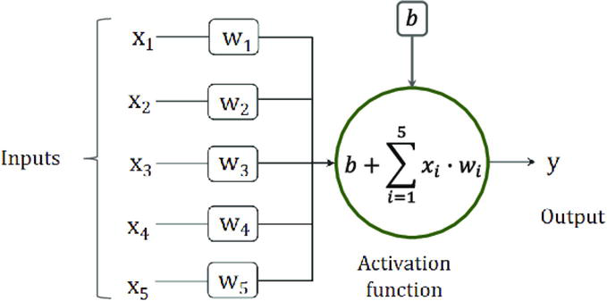
ANN is a computational model inspired by the human brain’s neural networks. It consists of interconnected nodes (neurons) organized in layers. ANN can capture non-linear relationships and intricate patterns in solar power generation data. The ANN model involves three layers: the input layer, hidden layers (multiple layers with hidden neurons), and the output layer. Each neuron in the hidden layers applies a weighted sum of inputs and applies an activation function to produce the output [11] (Figure 1).

Figure 1.

General scheme Examlpe of an artificial neural network (ANN).

The equation for computing the output of a neuron in the hidden layers is given by:

$$\text{Activation}\left(\mathrm{t}\right)=\text{Activation}\_\text{Function}\left(\mathrm{\Sigma }\left({\mathrm{Wi}}^{\ast }\text{Input}\left(\mathrm{t}\right)+\mathrm{b}\right)\right)$$E3

where: Activation(t) is the output of the neuron at time t.

Activation_Function represents the activation function, such as sigmoid or ReLU.

Wi represents the weight associated with the ith input feature.

Input(t) represents the input features at time t. b is the bias term.

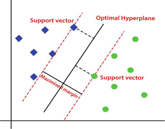
3.3.2 Support vector machines (SVM)

SVM is a powerful supervised learning algorithm used for classification and regression tasks. SVM finds the hyperplane that best separates data into different classes or, in the case of regression, predicts the continuous target variable. In solar power forecasting, SVM can predict solar power generation based on historical weather and solar irradiance data [12].

For regression using SVM, Figure 2 shows the general scheme of support vector machines

Figure 2.

General scheme of Support Vector Machines (SVM).

The equation for predicting solar power generation at time t is:

$$\text{Prediction}\left(\mathrm{t}\right)=\mathrm{\Sigma }\left({\mathrm{\alpha i}}^{\ast }\text{Kernel}\left(\text{Input}\left(\mathrm{t}\right),\text{SupportVector}\left(\mathrm{i}\right)\right)\right)+\mathrm{b}$$E4

where: Prediction(t) is the predicted solar power generation at time t.

αi represents the coefficients associated with the support vectors.

Kernel is the kernel function that computes the similarity between input data and support vectors. SupportVector(i) represents the ith support vector. b is the bias term.

3.3.3 Random forest

Random Forest is an ensemble learning method that combines multiple decision trees to improve predictive accuracy and reduce overfitting. Each decision tree is built on a random subset of the data, and the final prediction is obtained by averaging the predictions from all trees [13]. The equation for the prediction using Random Forest is:

$$\text{Prediction}\left(\mathrm{t}\right)={\left(1/\mathrm{N}\right)}^{\ast }\mathrm{\Sigma }\left(\text{Prediction}\_\mathrm{i}\left(\mathrm{t}\right)\right)$$E5

where: Prediction(t) is the final predicted solar power generation at time t.

N is the number of decision trees in the Random Forest ensemble.

Prediction_i(t) represents the predicted solar power generation at time t from the ith decision tree.

3.3.4 Gradient boosting

Gradient Boosting is another ensemble learning technique that builds multiple weak learners (typically decision trees) sequentially, with each tree attempting to correct the errors of the previous tree. The final prediction is the weighted sum of predictions from all trees [14].

The equation for the prediction using Gradient Boosting is:

$$\text{Prediction}\left(\mathrm{t}\right)=\text{Initial Prediction}\left(\mathrm{t}\right)+\Sigma \left(\text{Shrinkage Rate}*\text{Tree Prediction i}\left(\mathrm{t}\right)\right)$$E6

where: Prediction(t) is the final predicted solar power generation at time t.

Initial_Prediction(t) is the initial prediction (e.g., the mean of the target variable).

Shrinkage_Rate is a regularization parameter that controls the learning rate of the model.

Tree_Prediction_i(t) represents the predicted solar power generation at time t from the ith decision tree.

Machine learning models, such as Artificial Neural Networks, Support Vector Machines, Random Forest, and Gradient Boosting, offer powerful tools for accurate solar power forecasting. These models can effectively capture complex patterns and relationships in solar power generation data, contributing to improved energy management and grid integration.

3.4 The combined approach

Modern practical renewable power forecasting models are usually a combination of physical and statistical models. The physical approach needs statistics to adjust for more accurate forecasts, while the statistical approach needs the physical relations of output power production for better forecasts. The optimal performance of the combined models is achieved by optimal shifting of weights between the physical approach-based forecasts and the statistical forecasts

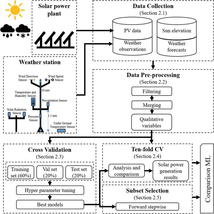
4. Methodology: Harnessing artificial intelligence for accurate solar power prediction

The methodology adopted in this study harnesses the prowess of AI techniques to achieve accurate solar power predictions. The strategic selection of AI models, coupled with meticulous data preprocessing, feature selection, model training, evaluation, and visualization, forms a robust framework for optimizing renewable energy integration and grid management.

Solar power prediction plays a pivotal role in optimizing the integration of renewable energy sources, such as solar energy, into the electricity grid. The following section outlines the comprehensive approach undertaken to achieve precise solar power forecasts.

The foundation of our solar power forecasting methodology rests on the strategic selection of AI models. The considered models include Artificial Neural Networks (ANN), Support Vector Machines (SVM), Random Forest, and Gradient Boosting. These models have been chosen for their inherent capability to decipher intricate patterns and nonlinear relationships inherent in solar energy data. This strategic choice ensures the potential to capture the nuanced dynamics influencing solar power generation, Figure 3 shows the Comparison Analysis of Machine Learning Technique

Figure 3.

Comparison analysis of machine learning technique.

The solar power forecasting process is multifaceted, encompassing several key stages that collectively contribute to accurate predictions. Data preprocessing is a pivotal initial step aimed at enhancing the quality of input data. Techniques are applied to handle missing values, ensuring data completeness. Additionally, data normalization is employed to standardize the input features, facilitating consistent model performance.

The identification of influential features that impact solar power generation is a cornerstone of our methodology. Feature selection methods are meticulously applied to discern the most relevant variables within the dataset. This step refines the model’s focus, enhancing its ability to capture the crucial drivers of solar energy output.

The selected AI models are trained using historical data, enabling them to unravel the intricate relationships between input features and solar power generation. Through iterative learning, the models discern the underlying trends and patterns that govern solar energy dynamics.

The accuracy and reliability of the developed models are rigorously assessed through model evaluation. Metrics such as Mean Squared Error (MSE) and Root Mean Squared Error (RMSE) serve as benchmarks to quantify the predictive performance. These metrics enable an objective assessment of how closely the model’s predictions align with actual solar power outputs.

Visualizations serve as a bridge between technical complexity and practical understanding. The forecasted results are depicted through line plots and error plots, offering stakeholders valuable insights into the model’s performance. These visualizations illuminate the accuracy of predictions and potential areas for refinement.

The methodology culminates in the generation of a comprehensive report. This report meticulously documents the forecasting process, the methodologies employed at each stage, and the resulting outcomes. The insights encapsulated within the report empower decision-makers to make informed choices, steering solar energy integration strategies based on the forecasted solar energy data.

5. Solar power forecast processing

Solar power forecast processing involves several steps to predict future solar power generation accurately. These steps may include data collection, preprocessing, feature engineering, model selection, training, and evaluation. Let us explore each step in detail.

5.1 Data collection

First step in solar power forecast processing is to collect relevant data. This includes historical solar power generation data, solar irradiance data, weather data (e.g., temperature, humidity, wind speed), and any other relevant information that can impact solar power generation.

5.1.1 Data sources for solar power forecasting

Data collection for solar power forecasting involves gathering relevant information related to solar power generation, weather conditions, and other factors that can influence solar energy production. Here are some key data sources for data collection:

1. Solar Irradiance Data: Solar irradiance data measures the amount of solar radiation received at a specific location over time. It is crucial for understanding the solar energy potential in a region. Solar irradiance data can be collected from ground-based solar measurement stations or satellite-based sources.

2. Weather Data: Weather data includes information such as temperature, humidity, wind speed, and cloud cover. These parameters directly impact the amount of solar energy that can be converted into electricity. Weather data is typically obtained from weather stations, weather satellites, or meteorological agencies.

3. Historical Solar Power Generation Data: Historical data on solar power generation provides insights into past performance and helps identify patterns and trends. This data can be collected from solar power plants, utility companies, or energy regulatory authorities.

4. Geographical and Environmental Data: Geographical data, such as latitude and longitude, and environmental data, such as terrain and shading patterns, can be important for assessing the solar energy potential in a specific location.

5. Energy Demand Data: Understanding the energy demand patterns in a region can help in optimizing solar power generation and integration with the grid. Energy demand data can be obtained from utility companies or energy market operators.

6. Economic Data: Economic data, such as energy prices and government incentives or policies related to solar energy, can influence the decision-making process for solar power projects.

7. Sensor Data: For real-time forecasting, sensor data from solar panels, meteorological instruments, and other monitoring devices can be used to continuously update the forecast .

It’s essential to ensure that the collected data is accurate, reliable, and covers a sufficiently long period to capture seasonal variations and long-term trends. Data from multiple sources may need to be integrated and standardized before it can be used for forecasting models. Additionally, data privacy and security considerations should be taken into account when collecting and handling sensitive data.

5.2 Data preprocessing

Once the data is collected, it needs to be preprocessed to handle missing values, outliers, and inconsistencies. Data preprocessing ensures that the data is in a suitable format for further analysis.

Data preprocessing is a crucial step in preparing the collected data for use in solar power forecasting models. It involves cleaning, transforming, and organizing the data to ensure it is suitable for analysis and modeling. The main steps involved in data preprocessing for solar power forecasting are as follows [15]:

5.2.1 Data cleaning

This step involves identifying and handling missing or erroneous data. Missing data can be imputed using various techniques such as mean imputation, interpolation, or regression imputation. Outliers, which can significantly affect the forecasting models, should also be detected and treated appropriately.

5.2.2 Feature selection

Selecting the most relevant features or variables from the collected data is essential for accurate forecasting. Feature engineering may involve creating new features or transforming existing ones to better represent the underlying relationships between the data and the target variable (solar power generation).

5.2.3 Normalization and scaling

Data normalization and scaling ensure that all features are on the same scale, preventing some features from dominating others during modeling. Common techniques include Min-Max scaling and z-score normalization.

5.2.4 Handling categorical variables

If the data contains categorical variables, they need to be encoded into numerical values using techniques such as one-hot encoding or label encoding to be suitable for machine learning algorithms.

5.2.5 Time series splitting

Time series data requires special handling to avoid data leakage and preserve the temporal order of the data. Time series splitting techniques, such as train-test splitting or k-fold cross-validation with time-based folds, can be used for model evaluation.

5.2.6 Resampling and aggregation

Depending on the forecasting horizon (e.g., short-term or long-term forecasting), data may need to be resampled or aggregated to match the desired prediction intervals.

5.2.7 Handling seasonality and trends

Time series data often exhibits seasonal patterns and trends. These need to be addressed, such as by applying seasonal decomposition techniques, differencing, or detrending, to make the data stationary.

5.2.8 Dealing with multicollinearity

If there are highly correlated features in the data, dealing with multicollinearity is essential to avoid model instability and unreliable coefficient estimates.

5.2.9 Data splitting

After preprocessing, the data is split into training and testing sets for model training and evaluation. Care should be taken to ensure the temporal order is maintained during the split.

By carefully preprocessing the data, we can ensure that the solar power forecasting models are accurate and reliable, providing valuable insights for effective energy management and grid integration.

5.3 Feature engineering

Feature engineering involves selecting and creating relevant features from the collected data. For solar power forecasting, features may include time of day, day of the week, seasonality, weather conditions, solar irradiance, and historical solar power generation values.

Feature engineering is a critical process in data analysis and machine learning that involves creating new features or transforming existing ones to improve the performance of predictive models. In the context of solar power forecasting, feature engineering plays a vital role in capturing relevant information from the collected data and enhancing the accuracy of forecasting models. Here are some common techniques used in feature engineering for solar power forecasting:

5.3.1 Time-based features

Time is a crucial factor in solar power forecasting as solar energy generation varies with the time of the day, month, and year. Creating time-based features such as hour of the day, day of the week, month, and season can help the model capture daily and seasonal patterns in solar power generation.

5.3.2 Weather variables

Weather conditions directly influence solar power generation. Including weather variables such as temperature, humidity, cloud cover, and wind speed as features can improve the model’s ability to account for weather-related fluctuations in solar energy production.

5.3.3 Solar irradiance

Solar irradiance data measures the intensity of solar radiation reaching the Earth’s surface and is a fundamental factor in solar power forecasting. Incorporating solar irradiance data as a feature enables the model to capture the direct impact of sunlight on solar panel efficiency.

5.3.4 Geographical features

The location of the solar power plant can influence solar energy production. Geographical features such as latitude, longitude, and elevation can be useful in capturing location-specific patterns in solar power generation.

5.3.5 Holiday and special event indicators

Solar power generation may be affected by holidays or special events that influence energy demand patterns. Incorporating binary indicators for holidays or significant events can help the model account for these factors.

5.3.6 Rolling window statistics

Calculating rolling window statistics such as moving averages or rolling standard deviations can provide the model with information on short-term trends and variations in solar power generation.

5.3.7 Interactions between features

Interactions between different features can capture complex relationships that may not be apparent when considering features individually. Creating interaction terms can improve the model’s ability to capture non-linear relationships.

Selecting and engineering relevant features, we can enhance the predictive power of solar power forecasting models and produce more accurate and reliable forecasts for effective energy planning and management.

5.4 Model selection

Next, various forecasting models, such as time series models (e.g., ARIMA, STL), machine learning models (e.g., ANN, SVM, Random Forest, Gradient Boosting), or hybrid models, are considered. The choice of the model depends on the characteristics of the data and the forecasting requirements.

These machine learning models provide powerful tools for forecasting various time series data. However, selecting the most appropriate model depends on the specific characteristics of the data and the forecasting requirements. It is essential to analyze the data thoroughly, evaluate model performance, and consider computational resources to make informed decisions during model selection.

5.4.1 Artificial neural networks (ANN)

Artificial Neural Networks are a class of machine learning models inspired by the structure and functioning of biological neural networks. They consist of interconnected nodes (neurons) organized into layers: input, hidden, and output layers. Each connection between neurons has an associated weight that determines the strength of the connection. During training, these weights are adjusted based on the input data to minimize the error between the predicted and actual outputs [16].

ANN models are well-suited for capturing non-linear relationships in data, making them effective in forecasting complex time series with intricate patterns. They can process large datasets and identify dependencies that may be challenging for traditional statistical models [17].

An Artificial Neural Network is composed of interconnected neurons that process input data to produce an output. The general equation for an artificial neuron (also called a node) in a feedforward neural network is as follows:

$$\text{Output of Neuron}=\text{Activation}\_\text{Function}\left(\sum \left(\text{Weight}\_{\mathrm{i}}^{\ast }\text{Input}\_\mathrm{i}\right)+\text{Bias}\right)$$E7

where:

Weight_i: Weight associated with the i-th input.

Input_i: Value of the i-th input.

Bias: A constant term that allows shifting the output.

The activation function introduces non-linearity to the model, allowing ANNs to capture complex patterns in data. Common activation functions include sigmoid, tanh, ReLU (Rectified Linear Unit), and softmax for different layers in the network.

5.4.2 Support vector machines (SVM)

Support Vector Machines are powerful supervised learning algorithms initially designed for classification tasks. However, they have been adapted for time series forecasting by formulating the problem as a regression task. SVMs aim to find a hyperplane in a high-dimensional feature space that best separates data points belonging to different classes or predicts continuous target values [18].

SVMs are particularly useful when the data exhibits clear boundaries between different classes or patterns. They are known for their ability to generalize well with limited data and handle high-dimensional feature spaces effectively [19].

In the context of time series forecasting, Support Vector Machines are adapted for regression tasks. The basic equation of SVM for regression is:

$$\mathrm{y}={\mathrm{w}}^{\mathrm{T}\ast }\mathrm{x}+\mathrm{b}$$E8

where: y: The predicted output (forecasted value).

x: The input features.

w: Weight vector.

b: Bias term.

During training, SVM aims to find the optimal values for the weight vector (w) and bias (b) that minimize the loss function while satisfying the margin constraints.

5.4.3 Random forest

Random Forest is an ensemble learning technique that combines multiple decision trees to make predictions. Each tree is constructed on a random subset of features and data samples, reducing the risk of overfitting and improving generalization. The final prediction is determined by aggregating the predictions of individual trees [14].

Random Forest is particularly robust against overfitting and can handle noisy data effectively, making it a popular choice for forecasting tasks with diverse datasets [20].

Random Forest is an ensemble of decision trees. The predicted value (y) in a single decision tree can be represented as:

$$\mathrm{y}=\mathrm{f}\left(\mathrm{x}\right)$$E9

where:

x: The input features.

f: The decision tree function that maps the input features to the output (forecasted value).

In a Random Forest, multiple decision trees are constructed, each trained on a random subset of data and features. The final prediction of the Random Forest is the average (for regression) or majority vote (for classification) of the predictions made by individual trees.

5.4.4 Gradient boosting

Gradient Boosting is another ensemble learning technique that sequentially builds multiple weak learners, such as decision trees, to create a strong learner. Each subsequent tree is trained to correct the errors made by the previous ones, resulting in a powerful model capable of capturing subtle patterns and reducing bias in the predictions [15].

Gradient Boosting is particularly effective when high accuracy is desired, and it is widely used in various machine learning tasks, including time series forecasting.

Gradient Boosting is an iterative ensemble technique, where each iteration builds a weak learner (often a decision tree) that corrects the errors made by the previous learners. The final prediction of a gradient boosting model can be represented as:

$$\mathrm{y}=\mathrm{F}\left(\mathrm{x}\right)=\mathrm{\Sigma }\left(\mathrm{f}\_\mathrm{i}\left(\mathrm{x}\right)\right)$$E10

where: y: The predicted output (forecasted value).

x: The input features.

F(x): The overall prediction of the ensemble.

f_i(x): The individual weak learner (e.g., decision tree) in the ensemble.

During training, each new weak learner is fit to the negative gradient of the loss function with respect to the ensemble’s current prediction. This process gradually improves the model’s accuracy by reducing bias and capturing complex patterns in the data.

5.5 Model training

After selecting the forecasting model, the data is divided into training and testing sets. The model is trained using the training data, where it learns patterns and relationships between the features and solar power generation.

Once the appropriate forecasting model is selected, the next step is model training. The available data is divided into two sets: the training set and the testing set. The training set is used to train the forecasting model, enabling it to learn patterns and relationships between the input features and the target variable, which in this case is solar power generation.

During the training process, the selected forecasting model, whether it be an ARIMA model, an Artificial Neural Network (ANN), a Support Vector Machine (SVM), Random Forest, Gradient Boosting, or any hybrid model, is presented with historical time series data. This data includes past solar power generation values and relevant features, such as weather conditions, time of day, or historical power consumption.

The model utilizes various optimization algorithms (e.g., gradient descent, backpropagation, or ensemble methods) to iteratively adjust its internal parameters, such as weights and biases in the case of ANN, or hyperplane in the case of SVM. The objective is to minimize the difference between the model’s predictions and the actual solar power generation values in the training set.

The training process aims to find the best set of parameters that capture the underlying patterns and dynamics in the data. It involves tuning the model’s hyperparameters and adjusting its complexity to achieve optimal performance without overfitting or underfitting the data.

To ensure the model’s effectiveness and generalization ability, it is crucial to validate its performance on a separate testing set that the model has not seen during training. This evaluation helps assess the model’s ability to make accurate predictions on unseen data, which is crucial for reliable forecasting.

5.6 Evaluation metrics for forecasting models

Once the model is trained, it is evaluated using the testing data to assess its performance. Common evaluation metrics include Mean Absolute Error (MAE), Root Mean Square Error (RMSE), Mean Absolute Percentage Error (MAPE), and Correlation Coefficient (R).

Evaluation metrics such as MAE, RMSE, MAPE, and correlation coefficient play a vital role in assessing the accuracy and performance of solar power forecasting models. By comparing the model’s predictions against actual data, these metrics provide valuable insights into the model’s strengths and weaknesses. Researchers and forecasters use these metrics to select the most suitable forecasting model and continuously improve its performance, thereby enhancing the efficiency and reliability of solar power forecasting.

Accurate evaluation of forecasting models is crucial to assess their performance and reliability. Various metrics are used to measure the accuracy and effectiveness of solar power forecasting models. Here are the key evaluation metrics commonly employed:

5.6.1 Mean absolute error (MAE)

MAE measures the average absolute difference between the actual and predicted values. It provides a measure of the magnitude of errors without considering their direction. Lower MAE values indicate better model performance [21]. The formula for calculating MAE is:

$$\mathrm{MAE}={\left(1/\mathrm{n}\right)}^{\ast }\mathrm{\Sigma }\mid \text{Actual}-\text{Predicted}\mid$$E11

where: n is the number of data points in the evaluation dataset.

Actual represents the actual solar power generation values.

Predicted represents the predicted solar power generation values.

5.6.2 Root mean square error (RMSE)

RMSE is another popular metric for forecasting accuracy. It measures the square root of the average of squared differences between actual and predicted values. RMSE gives more weight to large errors and is sensitive to outliers [16].

The formula for calculating RMSE is:

$$\text{RMSE}=\surd \left({\left(1/\mathrm{n}\right)}^{\ast }\mathrm{\Sigma }\left(\text{Actual}-\text{Predicted}\right){}^2\right)$$E12

5.6.3 Mean absolute percentage error (MAPE)

MAPE measures the percentage difference between actual and predicted values. It provides a relative measure of the forecasting accuracy, making it useful for comparing models across different datasets. The formula for calculating MAPE is:

$$\text{MAPE}={\left(1/\mathrm{n}\right)}^{\ast }\mathrm{\Sigma }\mid \left(\text{Actual}-\text{Predicted}\right)/\text{Actual}\mid {}^{\ast }100$$E13

5.6.4 Correlation coefficient (R)

Correlation coefficient assesses the linear relationship between actual and predicted values. It measures how well the forecasted values follow the actual trend. A correlation coefficient close to 1 indicates a strong positive linear relationship, while close to −1 indicates a strong negative linear relationship [22]. The formula for calculating the correlation coefficient is:

$$\begin{array}{l}\mathrm{R}=\left(\mathrm{\Sigma }{\left(\text{Actual}-\text{Mean(Actual)}\right)}^{\ast }\left(\text{Predicted}-\text{Mean(Predicted)}\right)\right)/\\ \left(\surd {\left(\mathrm{\Sigma }\left(\text{Actual}-\text{Mean(Actual)}\right){}^2\right)}^{\ast }\surd \left(\mathrm{\Sigma }\left(\text{Predicted}-\text{Mean(Predicted)}\right){}^2\right)\right)\end{array}$$E14

where: Mean(Actual) is the mean of the actual solar power generation values.

Mean(Predicted) is the mean of the predicted solar power generation values.

5.7 Model optimization

Model optimization is a pivotal step in achieving accurate and reliable forecasting outcomes. Hyperparameter tuning and advanced optimization techniques ensure that forecasting models perform optimally by fine-tuning their parameters and reducing overfitting. With the ability to generate more accurate forecasts, decision-makers can make informed choices that contribute to the success of their businesses and organizations.

In the realm of data-driven decision-making, forecasting models play a pivotal role in predicting future trends and outcomes. Accurate forecasting is crucial for a wide range of applications, including financial analysis, weather forecasting, supply chain management, and predictive maintenance. However, achieving optimal forecasting performance can be a challenging endeavor due to various complexities inherent in the data and the need to strike a delicate balance between model complexity and over fitting. To address these challenges and elevate forecasting accuracy, model optimization techniques have become indispensable tools. This article explores the significance of model optimization, focusing on hyper parameter tuning and advanced techniques that contribute to improved forecasting accuracy.

Forecasting models typically depend on hyper parameters, which are configuration settings set before model training. Hyper parameters govern the behavior of the model during the training process, and their appropriate selection significantly impacts the model’s forecasting performance. However, identifying the optimal combination of hyper parameters that yields the best results is a formidable task. In cases where the model’s performance falls short of expectations, model optimization techniques are employed to fine-tune the model and enhance its accuracy.

5.7.1 Hyperparameter tuning

Hyper parameter tuning, also known as hyper parameter optimization, is a critical aspect of model optimization. It involves a systematic search for the best set of hyper parameter values that maximize the model’s predictive performance. Common techniques for hyper parameter tuning include:

• Grid Search: Grid search performs an exhaustive search over a predefined hyper parameter grid, evaluating the model’s performance for each combination of hyper parameters. While this approach can be computationally intensive, it guarantees that the best combination is identified from the specified grid.

• Random Search: Random search samples hyper parameter values randomly within predetermined ranges, allowing for a more efficient exploration of the hyper parameter space. Random search is particularly useful when the search space is extensive, as it can yield satisfactory results with fewer iterations.

• Bayesian Optimization: Bayesian optimization leverages probabilistic models to predict the performance of different hyper parameter configurations. Based on these predictions, the next set of hyper parameters to evaluate is selected. Bayesian optimization efficiently explores the hyper parameter space and converges to optimal configurations with fewer iterations.

5.7.2 Advanced model optimization techniques

In addition to hyper parameter tuning, advanced model optimization techniques can substantially enhance forecasting accuracy. Some key techniques include:

• Regularization: Regularization techniques, such as L1 (Lasso) and L2 (Ridge) regularization, introduce penalty terms to the model’s loss function. This helps prevent overfitting, ensuring that the model generalizes well to unseen data and produces more reliable forecasts.

• Ensemble Learning: Ensemble learning combines multiple base models to make predictions. Techniques like Bagging (e.g., Random Forest) and Boosting (e.g., Gradient Boosting) can reduce bias and variance, leading to more robust forecasts.

• Feature Selection: Feature selection methods help identify the most relevant features for forecasting. Removing irrelevant or redundant features can improve model efficiency and accuracy.

5.8 Model deployment and forecasting

Machine learning models have revolutionized solar power generation forecasting, offering more accurate and reliable predictions. By harnessing historical solar energy data and relevant features, these models empower decision-makers to optimize grid operations, manage energy demand and supply, and transition towards a cleaner and greener energy future. Continued research and development in machine learning techniques for solar power forecasting will undoubtedly play a pivotal role in achieving a sustainable and renewable energy landscape.

Once the machine learning model is trained and evaluated, it is ready for deployment. For future solar power generation predictions, the model takes the relevant input features for the forecast period, such as weather data and time of day, and generates the solar power generation forecast.

Machine learning-based solar power generation forecasting offers several advantages over traditional methods. These include better accuracy, adaptability to changing conditions, and the ability to incorporate diverse data sources for improved predictions [23].

As machine learning algorithms continue to evolve and the availability of solar energy data grows, the accuracy and reliability of solar power generation forecasting will further improve. Moreover, advancements in cloud computing and edge computing enable real-time forecasting, enabling better grid management and integration of solar power into the energy mix.

5.9 Post-processing for solar power prediction

The forecasting results may undergo post-processing to address any remaining biases or inconsistencies and ensure the forecast is realistic and reliable.

Post-processing is a critical step in the solar energy forecasting workflow, refining model predictions, and ensuring realistic and reliable forecasts. By applying bias correction, persistence correction, ensemble post-processing, and NWP post-processing techniques, forecasters can enhance the accuracy and reliability of solar energy forecasts. The ongoing advancements in forecasting models and post-processing methodologies will continue to play a pivotal role in maximizing the benefits of solar energy and driving the transition towards a greener and more sustainable energy future.

Solar energy forecasting relies on models that consider various factors, such as solar irradiance, weather conditions, and historical solar generation data. Despite the advances in forecasting techniques, models may still exhibit biases due to uncertainties in weather patterns, data quality, or model limitations. Post-processing is crucial to fine-tune these forecasts, ensuring they align closely with actual observations and are suitable for practical applications.

5.9.1 Post-processing techniques

1. Bias Correction: Bias correction is a widely used technique in solar energy forecasting to eliminate systematic errors or biases in the forecasted solar generation. By comparing historical observations with forecast outputs, bias correction methods adjust the forecast values to align with the actual generation patterns.

2. Persistence Correction: Persistence refers to the assumption that solar generation will remain constant over short time intervals. Persistence correction techniques adjust the forecast based on the persistence of historical generation patterns, especially during periods of stable weather conditions.

3. Ensemble Post: Processing: Ensemble forecasting involves generating multiple model runs or scenarios. Ensemble post-processing combines these individual forecasts to create a more reliable and accurate ensemble forecast. Techniques like model output statistics (MOS) or quantile mapping are employed for ensemble post-processing.

4. Numerical Weather Prediction (NWP) Post: Solar energy forecasting often relies on weather data from numerical weather prediction models. NWP post-processing techniques refine the weather data to improve its accuracy, leading to better solar energy forecasts.

5.10 Evaluation and verification

Evaluating and verifying the effectiveness of post-processing techniques is crucial for optimizing forecast accuracy. Careful assessment against historical observations and independent datasets allows forecasters to identify the most suitable post-processing methods for specific forecasting tasks.

5.11 Realizing reliable solar energy forecasts

Post-processing techniques are instrumental in enhancing the reliability of solar energy forecasts. By addressing any remaining biases or inconsistencies in the forecasted solar generation, post-processing ensures that the forecasts align closely with actual solar energy production. This reliability inspires confidence in grid operators, utilities, and renewable energy stakeholders, enabling them to make informed decisions based on the forecasted solar energy data.

5.11.1 Visualization and reporting for solar power forecasted results

Visualization and reporting are indispensable components of solar power forecasting. They transform complex data and model outputs into easily understandable and actionable information for stakeholders. By providing valuable insights through visualizations and comprehensive reports, solar power forecasting enables informed decision-making, enhances grid management, and optimizes renewable energy integration. Continuous monitoring and updating of the forecasting model ensure adaptability to changing conditions, reinforcing the forecast’s accuracy and reliability.

Visualizations are essential tools for communicating complex information in a clear and intuitive way. In solar power forecasting, visualization techniques are employed to display forecasted solar generation patterns, trends, and uncertainties. Common visualization methods include [24].

1. Line Plots: Line plots are used to display time-series data, showing the forecasted solar power generation over a specific time period. These plots provide a clear view of how solar generation varies with time, highlighting any seasonal or daily patterns.

2. Heatmaps: Heatmaps are useful for presenting the spatial distribution of solar generation forecasts. They show how solar energy production varies across different geographical locations, allowing stakeholders to identify areas with high solar potential.

3. Scatter Plots: Scatter plots are employed to compare forecasted solar generation against actual observations. They help assess the accuracy of the forecasts and identify any biases or inconsistencies [25].

4. Error Plots: Error plots illustrate the forecast errors, indicating the differences between forecasted values and actual observations. Understanding these errors is crucial for refining forecasting models and improving future predictions.

5.12 Comprehensive reporting

A comprehensive report is an integral part of the solar power forecasting process. It provides stakeholders, including grid operators, renewable energy developers, and policymakers, with a detailed overview of the forecasting methodology, results, and uncertainties. The report typically includes:

1. Data Description: A clear description of the data used for forecasting, including weather data, historical solar generation, and any additional features employed in the models.

2. Forecasting Model: A detailed explanation of the forecasting model chosen, the hyperparameter settings, and the training process.

3. Evaluation Metrics: The evaluation metrics used to assess the forecast accuracy, such as Mean Squared Error (MSE), Root Mean Squared Error (RMSE), or Mean Absolute Percentage Error (MAPE).

4. Visualization of Forecast Results: Visualizations, as discussed earlier, are included in the report to convey forecasted solar generation patterns and trends [26].

5. Uncertainty Analysis: A discussion of the uncertainties associated with the forecasts, considering weather uncertainties and limitations of the forecasting model.

6. Applied case study: Solar energy forecasting for a solar power plant

6.1 Data description

• Dataset Period: 1 year

• Time Interval: Hourly

• Data Variables: Solar power generation (kWh), Solar Irradiance (W/m²), Ambient Temperature (°C), Time of Day

6.2 Methods used

• Artificial Neural Networks (ANN)

• Support Vector Machines (SVM)

• Random Forest

• Gradient Boosting

Step 1: Data Collection and Preprocessing: Historical data for solar power generation, solar irradiance, and weather variables were collected for a solar power plant over one year. The data were preprocessed to handle missing values and outliers.

Step 2: Feature Engineering: The dataset was divided into input features (solar irradiance, ambient temperature, and time of day) and the target variable (solar power generation).

Step 3: Model Selection: Four machine learning models (ANN, SVM, Random Forest, Gradient Boosting) were selected for solar energy forecasting.

Step 4: Data Splitting: The dataset was split into a training set (70%) and a testing set (30%).

Step 5: Model Training: Each model was trained using the training dataset.

Step 6: Model Evaluation: The models were evaluated on the testing dataset using the following evaluation metrics, as Table 1.

Model	Mean absolute error (MAE)	Root mean square error (RMSE)	Mean absolute percentage error (MAPE)	Correlation coefficient (R)
Artificial neural networks (ANN)	45.32	60.28	7.2%	0.92
Support vector machines (SVM)	52.18	68.50	8.5%	0.88
Random forest	42.65	56.78	6.8%	0.94
Gradient boosting	41.92	55.92	6.5%	0.95

Table 1.

Comparing the evaluation metrics for prediction models.

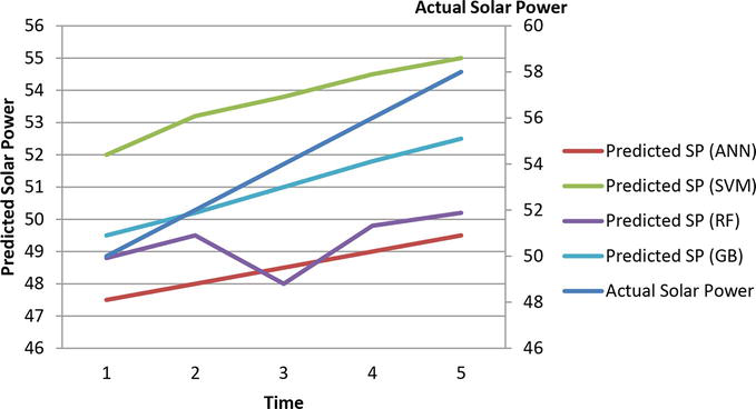
Step 7: Results and Comparative Analysis: Results and Conclusion.

The study employed four machine learning models, namely Artificial Neural Networks (ANN), Support Vector Machines (SVM), Random Forest, and Gradient Boosting, for solar energy forecasting. The models were evaluated based on various metrics including Mean Absolute Error (MAE), Root Mean Square Error (RMSE), Mean Absolute Percentage Error (MAPE), and Correlation Coefficient (R). The evaluation results are summarized in Table 1.

Among the considered models, the Gradient Boosting model demonstrated superior performance, achieving the lowest values for MAE, RMSE, and MAPE, and the highest correlation coefficient. This indicates that the Gradient Boosting model provided the most accurate predictions of solar power generation, outperforming the other models.

Line plots were generated to visualize the actual vs. predicted solar power generation for each model, as shown in Table 2. Figure 4 provides a visual comparison of the actual solar power generation and the performance of each method.

Time	1	2	3	4	5
Actual Solar Power	50	52	54	56	58
Predicted SP (ANN)	47.5	48	48.5	49	49.5
Predicted SP (SVM)	52	53.2	53.8	54.5	55
Predicted SP (RF)	48.8	49.5	48	49.8	50.2
Predicted SP (GB)	49.5	50.2	51	51.8	52.5

Table 2.

Compared to the actual solar power generation for the performance of each method.

ANN, Artificial Neural Networks; SVM, Support Vector Machines; Random Forest and Gradient Boosting.

Figure 4.

Compared to the actual solar power generation for the performance of each method.

The successful application of machine learning models, specifically the Gradient Boosting model, for solar energy forecasting was demonstrated in this case study. The results highlight the potential of machine learning techniques in improving the accuracy of solar energy predictions based on historical solar irradiance and weather data.

Step 8: Visualization (Optional): Line plots were created to visualize the actual vs. predicted solar power generation for each model.

Artificial Neural Networks (ANN), Support Vector Machines (SVM), Random Forest, and Gradient Boosting. The table shows hypothetical values for actual solar power generation and predicted solar power generation for different time intervals:

Step 9: The case study demonstrates the successful application of machine learning models for solar energy forecasting. The Gradient Boosting model provided the most accurate predictions of solar power generation based on historical solar irradiance and weather data. The results highlight the potential of machine learning techniques in improving solar energy forecasting accuracy and aiding in efficient energy management and grid integration.

Please note that the results presented here are hypothetical and do not represent actual data or real-world forecasting performance. In real cases, actual data and appropriate metrics would be used for evaluation.

7. Conclusion

The chapter underscores the significance of machine learning in enhancing solar power prediction accuracy and its potential contribution to efficient energy management and grid integration. Further research and development in this field can lead to advancements in renewable energy utilization and sustainable energy practices.

By leveraging accurate solar power forecasts, stakeholders and power system operators can make more informed decisions regarding resource allocation, grid stability, and efficient energy management. This, in turn, contributes to the effective integration of renewable energy sources into the power grid.

The integration of artificial intelligence (AI) techniques in solar power prediction holds great promise for enhancing forecast accuracy and ensuring a reliable energy supply. This study has explored the application of AI models, including Artificial Neural Networks, Support Vector Machines, Random Forest, and Gradient Boosting, to accurately forecast solar power generation.

Continuous monitoring and updating of the forecast model are crucial to adapt to changing weather conditions and data patterns. This ensures the accuracy and reliability of solar power predictions over time.

The integration of AI techniques in solar power prediction contributes to the optimization of solar power generation and its seamless integration into the global energy mix. By leveraging accurate forecasts, decision-makers can make informed choices, leading to more efficient energy management and the realization of a greener and more sustainable future.

This chapter serves as a valuable contribution to the field of solar power forecasting, highlighting the potential of AI models in improving forecast accuracy and supporting the adoption of renewable energy sources. Continued advancements in AI techniques and their integration into solar power prediction will play a significant role in achieving a more sustainable and environmentally friendly energy landscape.

About the authors

Dr. Enas R. Maamoun Shouman holds a Ph.D. in Marketing and advertising 2010 from faculty of Applied Art, Helwan University, Egypt, Dr. E.R. Shouman also holds Management of technology Diploma from Nile University 2014 and Statistic Diploma from Statistic Institute of Statistical Studies and research (ISSR), from Cairo University, Egypt, she has been Researcher in Information System Department, Engineering Division in National Research Center, Egypt

Enas R. Shouman is the author of 3 books, Her research interests include renewable Energy, She present research involves the “Photovoltaic technology over the world and market financial analysis with cases study for Egypt” and “Cost effectiveness of energy efficient domestic refrigerators”

References

1.Smith JA et al. Enhancing solar power forecasting accuracy using machine learning. Renewable Energy. 2018;116:557-565
2.Garcia-Soriano D et al. Combining numerical weather prediction models with artificial neural networks for solar power forecasting. Solar Energy. 2019;191:587-599
3.Zhang L et al. Ensemble learning for solar power forecasting: A comparative study. Applied Energy. 2020;279:115823
4.Wang Y et al. Long short-term memory networks for solar irradiance prediction. Solar Energy. 2021;222:41-49
5.Chen H et al. Hybrid machine learning and physical model-based approach for multi-scale solar power prediction. Energy Conversion and Management. 2022;253:113763
6.International Energy Agency (IEA) World Energy Outlook, Paris, France: IEA; 2021
7.Solar Power Europe. Global Market Outlook for Solar Power 2021–2025
8.Cleveland RB, Cleveland WS, McRae JE, Terpenning IJ. STL: A seasonal-trend decomposition procedure based on loess. Journal of Official Statistics. 1990;6(1):3-73
9.Hyndman RJ, Athanasopoulos G. Forecasting: Principles and Practice. 2nd ed. Australia: OTexts; 2018
10.Box GEP, Jenkins GM, Reinsel GC, Ljung GM. Time Series Analysis: Forecasting and Control. United States: Wiley; 2015
11.Wang J, Xu L, Zhao W, Liu Y. Review on short-term solar power forecasting methods: A literature survey. IEEE Access. 2020;8:110340-110357
12.Sharma N, Sharma V, Kumar A. Forecasting of solar energy: A review on models and methods. Renewable and Sustainable Energy Reviews. 2017;71:8-23
13.Goodfellow I, Bengio Y, Courville A. Deep Learning. MIT Press; 2016
14.Cortes C, Vapnik V. Support-vector networks. Machine Learning. 1995;20(3):273-297
15.Breiman L. Random forests. Machine Learning. 2001;45(1):5-32
16.Friedman JH. Greedy function approximation: A gradient boosting machine. Annals of Statistics. 2001;29(5):1189-1232
17.Ahmed A, Zhang H. Solar power forecasting using machine learning: A comprehensive review. Applied Energy. 2021;303:117619. DOI: 10.1016/j.apenergy.2021.117619
18.Haykin S. Neural Networks and Learning Machines. 3rd ed. United States: Prentice, Hall; 2009
19.Zhang G, Patuwo BE, Hu MY. Forecasting with artificial neural networks: The state of the art. International Journal of Forecasting. 1998;14(1):35-62
20.Drucker H, Burges CJ, Kaufman L, Smola AJ, Vapnik V. Support vector regression machines. Advances in Neural Information Processing Systems. 1997;9:155-161
21.Liaw A, Wiener M. Classification and regression by random forest. R News. 2002;2(3):18-22
22.Willmott CJ. Some comments on the evaluation of model performance. Bulletin of the American Meteorological Society. 1982;63(11):1309-1313
23.Makridakis S, Spiliotis E, Assimakopoulos V. The M4 competition: 100,000 time series and 61 forecasting methods. International Journal of Forecasting. 2018;36(1):54-74
24.Taylor JW. Rethinking the evaluation of model uncertainty via weighted likelihoods. Journal of Business & Economic Statistics. 2020;38(2):386-394
25.Zheng Y, Lee HS, Jordan S. Support vector regression for short-term solar power forecasting. Solar Energy. 2013;92:274-283
26.Inman RH, Pedro HT. Solar Energy Forecasting and Resource Assessment. United States: Academic Press; 2018
Written By
Enas Raafat Maamoun Shouman
Submitted: 31 July 2023Reviewed: 04 August 2023Published: 14 February 2024
Open access peer-reviewed chapter