State-Space Modeling of Weld Bead Geometry in the Gas Metal Arc-Direct Energy Deposition Process Applied to Wire and Arc Additive Manufacturing and Welding Processes

Abstract

One of the main problems of additive manufacturing with electric arc and welding, in general, is the difficulty in controlling or predicting the output variables and their parameters, as well as creating a model that effectively represents the changes in the main variables involved in the system. These changes during the deposition process can promote the formation of splashes, instabilities, and changes in the geometry of the beads, making the analysis of these variables important, as it will be through them that the quality of the deposit and the desired characteristics will be established. Despite the correlation between the variables, they present nonlinear and chaotic behavior. With this, the purpose of this research is mathematical modeling in state space that allows an approximation to the model in state spaces, an approximation of the real values of the process, and a knowledge of the system composed of a set of input, output, and states related to each other by means of first-order differential equations. The model was validated from depositions via a design of experiments with central composite planning monitored with the use of sensors to capture the characteristics of the beads (e.g., molten pool, width, penetration, and height).

1. Introduction

The model constitutes an abstract representation of a certain aspect of reality. In its structure, the elements that characterize the modeled reality intervene in the existing relationships between them. A mathematical model is a model based on mathematical logic, whose elements are essentially variables and functions, and the relationships between them are expressed through equations, inequalities, logical operators, state space, vectors, or matrices that correspond to the real relationships that can be modeled (technological relationships, physical laws, forces, time-varying population, financial, or market quantities) [1].

Some of the models presented in the literature are complex, having an exacerbated number of input data and difficult-to-solve equations, thus promoting, for control or identification, high processing time, and high computational cost [2]. Other simplified models present shorter processing times, but do not approach the reality of the phenomenon involved as required. This becomes a problem when you want to obtain acceptable information with a high speed in data processing. The main objective in predicting any physical phenomenon and an important part of the present work is to develop a mathematical model that allows describing and predicting the behavior of this phenomenon and preferably with simplified equations [3]. In the present work, it is important to learn and mathematically model the phenomena that involve the physics of the arc in the welding process, such as, the values of reinforcement width and penetration using the GMAW welding technique [4, 5].

For control engineering, any dynamic, time-varying, or time-invariant physical system can have a state-space representation. The state-space model is a mathematical model of a physical system composed of a set of input, output, and state variables related to each other through first-order differential equations. Variables are expressed in vectors and differential and algebraic equations can be written in matrix form when the dynamical system is linear and time invariant. The state-space representation with a time-domain approach provides a practical and compact way to model and analyze systems with multiple inputs and outputs. In the frequency domain, the use of the state-space representation is not limited to systems with linear components and zero initial conditions. The “state space” refers to the space whose axes are the state variables. The state of the system can be represented as a vector within this space [1].

2. State-space modeling

The proposal in this item is to develop a mathematical model by state space, that is, a dynamic model that can: predict the desired output variables; generalize to different operating points in working ranges in globular and droplet mode; and predict the proposed outputs, width, reinforcement and penetration through input values by the state variables used for control.

2.1 Definition of variables

In order to achieve a complete study of the phenomenon, eight states proposed for output prediction were used: width, reinforcement, and penetration. Next, Table 1 describes the proposed states, the type of measurement made in each of the variables (Online or Offline), the units used, and the sensor or sensors with which the measurement was performed.

Symbol	Variable	Unit	Measurement type	Sensor or technique used
X1: $\mathit{ls}$	Stick out	(mm)	Offline	Shadowgraph
X2: Ia	Current	(A)	Online	Ammeter
X3: Ws	Wire feed speed	(m/min)	Online	Encoder on feeder motor
X4: Cs	Solid wire length	(mm)	Online	Shadowgraph
X5: Ts	Travel speed	(mm/s)	Online	Encoder in linear table motor
X6: Wb	Bead width	(mm)	Online	Infrared Camera Scanner
X7: R	Reinforcement	(mm)	Online	Infrared Camera Scanner
X8: P	Penetration	(mm)	Online	Macrograph

Table 1.

State variables with the type of measurement and the sensor with which it was measured.

The input variables for the control are U1, U2, and U3 and their details are shown in Table 2.

Variable	U1—Uoc	U2—Uma	U3—Ums
Detailing	Voltage applied by the source (V)	Voltage applied across motor armature to obtain Ws (V)	Voltage applied to motor armature to obtain Ts (V)
Measurement	On-line	On-line	On-line
Sensor	Voltmeter	Voltmeter—Ratio between the load on the motor and the wire feed speed	Voltmeter—Relationship between the load on the motor and the speed of the linear displacement table that contains the part to be welded

Table 2.

Input variables.

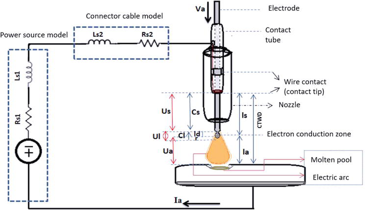
For the purposes of formulating the mathematical model by state space, a first study is presented, based on equations taken from other works in the field of arc physics and some considerations of our own. For this case, using a mathematical model, there is greater complexity when working in short circuit together with other transfer modes, which is why in this research proposal the droplet mode will be the focus, given the difficulty of working with several modes of transfer in the same model, considering models developed for GMAW such as the Moore, Naido and Tayler model [6], Thomsen [7] and Plankaert, Djermoune, Brie and Richard [8]. The plant of the system can be proposed for this research as shown in Figure 1 and the variables detailed in Table 3.

Figure 1.

Welding plant and its main electrical components.

Variable	Description
la	Arc length
CTWD	Contact to work distance
ls	Stick out
Cs	Wire length in solid state
Cl	Wire length in liquid state
ld	Drop Offset—distance from the solid wire to the center of the drop
h	Distance from the center of the drop to the conduction zone on the Y axis = rd cos(θ)
r	Distance from droplet tip to conduction zone
re	Electrode radius
rd	Drop radius
θ	W.t; where t is time and W is a constant representing the angular frequency in rad/s which relates to various factors that determine drop growth.
Us	Voltage drop in solid wire
Ua	Arc voltage drop
Ul	Voltage drop in liquid wire
Uoc	Open circuit voltage drop = sum of voltage drops in the system
Ls1	Inductance generated at the source
Ls2	Inductance generated in the cable
Rs1	Resistance inside the source
Rs2	Cable resistance
Ia	Current flowing in the cable
Ws	Wire feed speed
d	Length between the end of the wire and the part

Table 3.

Welding plant variables used to formulate the mathematical model.

The current presents different oscillations, the explanation of these oscillations working with the source at constant voltage is due to the growth of the drop and changes in the conduction zone. This is because for higher values of current and fusion energy, the drop size decreases and its detachment frequency increases. Various techniques were used to see changes in arc length, droplet size, and droplet detachment frequency. Many of these techniques use infrared cameras, optical filters, digital filters, high-speed cameras, algorithms for data processing, among other tools. Making use of experimental data collected in the tests, based on images and videos taken with the different techniques mentioned, an analysis was made of how these variables change, such as the length of arc and wire, subsequently managing to relate them to the input and output parameters when proposing the state equations; therefore, in this first step, the influence of the growth and detachment of the drops in the total system will be introduced and some equations are proposed, which will help to understand the proposed state system. For this, was approached an analysis of droplet formation and arc length.

2.2 Analysis of droplet formation and arc length

In the first observations when performing changes in voltage, current, and wire speed, the videos show records of a change in droplet size and frequency of droplet detachment. The reverse also happens where changing the droplet and its frequency affects the current, due to changes in the arc length and the resistance in the arc that the droplet generates. Thus, for higher values of current and fusion energy, the drop size decreases and its detachment frequency increases. This causes the current signal to also present a smaller oscillation in its signal intensity changes, but happening with greater frequency.

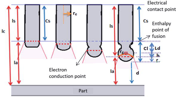
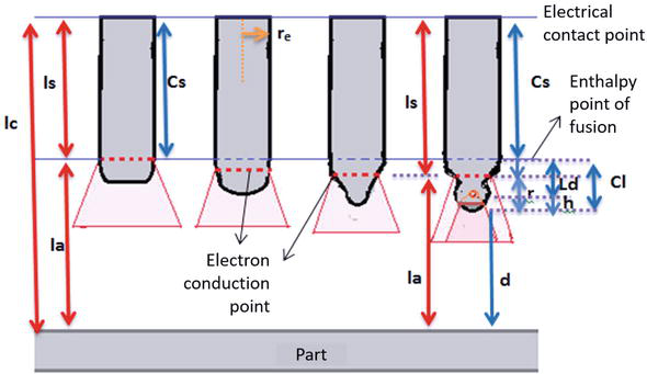
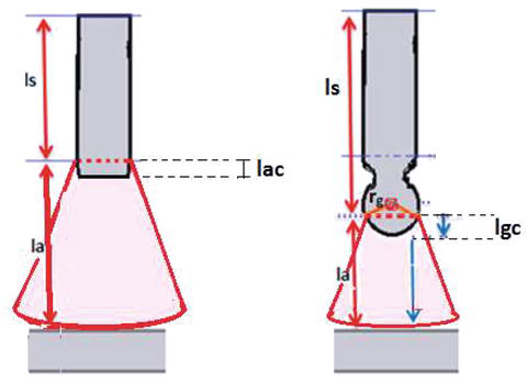
In most models, values work where the radius of the drop is proportional to the radius of the wire, that is, in the transition from globular to droplet, where the conduction zone (h) is below the center of the drop, at a distance h = re.cosθ, where re is the electrode radius. But for higher values of current and voltage above the transition point, the droplet has a smaller size, and at the same time increases the anodic zone in the electrode and the conduction zone, with which this conduction zone appears above the center of the drop as evidenced in some images of the welding process shown in Figures 2 and 3 and visualized in the images captured experimentally in Figure 4 by different capture methods. Trying to determine the geometry of the plasma, the length of the arc and the location of the wire and drop. Another point to consider is the high frequency in the formation of drops, this short time makes the oscillation in the current to be minimal, as well as its arc length.

Figure 2.

Behavior of the conduction zone during droplet formation at the globular transition point—Droplet with droplet equal to the wire size.

Figure 3.

Behavior of the conduction zone during drop formation for high current and voltage values.

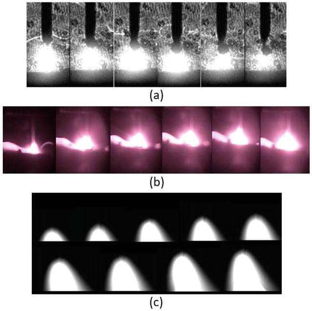
Figure 4.

(a) Plasma and wire visualized with shadowgraph at high voltages during drop formation and detachment. (b) Voltage increments for viewing the plasma with the infrared camera. (c) Voltage increments to visualize plasma only using optical bandpass filter between 625 and 700 nm and a high-speed camera.

Changes in arc length due to droplet formation introduce noise into the system due to the change in arc voltage drop. The relationships between the lengths are (Eqs. (1)–(3)):

$$l_a=\mathit{\text{CTWD}}-\mathit{ls}$$E1

$$\mathit{ls}=\mathit{Cs}+l_d+\mathrm{h}=\mathit{Cs}+l_d+r_{d}cos\left(\theta \right)$$E2

$$l_a=d+r$$E3

This value of r can be considered approximately equal to the displacement of the droplet in droplet mode. The electrode length in the solid state shows dynamic variation dependent on the wire feed speed (Ws), in addition to the melt volume rate ($\dot{\mathit{VfR}}$). Such behavior can be represented below (Eq. (4)).

$$\frac{\mathit{dCs}}{\mathit{dt}}=W_s-\frac{\dot{\mathit{VfR}}}{\pi {r_e}^2}$$E4

Where:

$\dot{\mathit{VfR}}$ = Melted volume per unit time.

Ws = Wire feed speed.

Substituting Eq. (4) by the variables of the state model we have (Eq. (5):

$$\frac{\mathit{dX}4}{\mathit{dt}}=\mathrm{X}3-\frac{\dot{\mathit{VfR}}}{\pi {r_e}^2}$$E5

The electrode is molten, constantly adding liquid metal to the drop that is forming at the tip of the electrode. The change in the mass of the drop ($m_d)$ is directly influenced by the melting rate of the electrode, as evidenced in the following equation (Eq. (6)):

$$\frac{d{m}_d}{\mathit{dt}}=\dot{\mathit{VfR}}\ast {\rho }_e$$E6

The length of the electrode $\left(h\right)$ between the torch and the weld pool depends on the difference between the wire feed speed and the molten portion of the wire when a certain voltage is applied, which allows to maintain a balance between the molten material rate and the length distance of bow (Eq. (7)).

$$\frac{\mathit{dh}}{\mathit{dt}}=\frac{\dot{{\mathit{Vf}}_R}}{A}\mathrm{ou}h=\frac{{\mathit{Vf}}_R}{A}$$E7

Where $\dot{\mathit{VfR}}$ is the volumetric melting rate of the electrode per unit time and A constitutes the area of the electrode (Eq. (8)).

$$A=\pi {r_e}^2$$E8

Therefore, when dividing $\dot{\mathit{VfR}}$ using area A, a value for the length of molten wire per unit of time (h) is obtained. The melting rate of the electrode is due to the influence of two factors, namely: ohmic and anodic heating. The melting rate of the electrode varies depending on the intensity of the current, the type of material, and the gas used, and this results in an equation that depends on the current and that for each material and gas used presents constants C1 and C2 (Eqs. (9) and (10)).

$${\mathit{Vf}}_R=C_{1}I+C_2{I}^2{\mathit{\rho l}}_s$$E9

Substituting for the state variables, the result is:

$${\mathit{Vf}}_R=C_1{X}_2+C_2{X_2}^2{\mathit{\rho X}}_1$$E10

Another relationship for the molten volume per unit time comes from Eq. (11) or Eq. (12):

$$\mathrm{d}{\mathit{Vf}}_R=A.W_s.\mathit{dt}$$E11

$${\mathit{Vf}}_R=A.W_s.t$$E12

Where A is the area of the electrode or wire. The volume melted per unit time always equals the volume added per unit time. When you increase or decrease the voltage and current, you increase or decrease the arc length, compensating for the heat to fuse the wire and stabilizing the entire system. There is a great influence of the inductance that is related to the variation of the current and the applied voltage, as well as a relationship of the resistance of the given source and the current that is circulating in the system as exposed in the Eq. (13).

$$L_s\frac{\mathit{dI}}{\mathit{dt}}+\left(R_f+R_a\right)I+U_a=U_{\mathit{oc}}$$E13

Where:

Ls = Sum of total inductance in the system $L_s=\frac{\mathit{Ls}1\ast \mathit{Ls}2}{\mathit{Ls}1+\mathit{Ls}2}$.

Rf = System resistance without taking into account the arc resistance.

Rf = R_s1 + R_s2.

Rs = Rf + Ra.

Ua = Arc voltage drop.

Uoc = Voltage at the source output.

Arc voltage and resistance are related to voltage drops. A strong relationship between arc voltage, arc length, and arc current is also shown. In the transition range from globular to droplet mode, where the drop has a radius equal to the size of the wire radius, the conduction zone was calculated performing an approximation only with the volumes and calculating the value of the conduction wire length (lac). For this relationship, the volume of the wire is considered as a cylinder, the spherical drop with a radius equal to the radius of the cylinder with a ratio between the volume of the drop and the volume of the cylinder of 3∕2 (Figure 5).

Figure 5.

Scheme of the plasma shape during the formation of a droplet at the transition point (when rg = re droplet mode), with arc length variation (la) and conduction zone.

Based on Figure 5 and previous analyses, Eq. (14):

$$\frac{1}{3}.V_g=A\ast l_{\mathit{ac}}$$E14

Respecting $V_g$ is the volume of the drop and that the voltage and current have values where the radius of the drop is equal to the radius of the electrode and later isolating $l_{\mathit{ac}}$ we get the value of the wire length of the conduction zone at the transition point, $l_{\mathit{ac}}=0.267\mathit{mm}.$ Experimentally, it is observed that there is no linear or quadratic variation in $l_{\mathit{ac}}$ as the voltage increases, so it is proposed to apply a 3/2 exponent that matches the experimental data and add the corresponding constants of proportionality. With the application of these proposed equivalences, the equation for the length of the wire in electrical conduction finaly looks like this (Eq. (15)):

$$l_{\mathit{ac}}=\frac{\left(C7\ast e^{0.38\ast {\left(\mathit{Uoc}-\mathit{Ut}\right)}^{\frac{1}{3}}}-C9\ast {l_a}^{\frac{3}{2}}\ast r_e-\mathrm{C}10\right)}{\pi \ast {r_e}^2}$$E15

Where Uoc is the output voltage of the source, Ut is the voltage at the transition point for this wire and gas used, which experimentally obtained Ut = 26.5 V for pure argon, and for argon with 4% CO2 Ut = 23 V. Then continue using the values with 4% CO2. And finally the constants C7, C9, and C10, are system constants that have been found experimentally. Substituting the constants and the Ut value, the conduction length finally looks like this (Eq. (16)):

$$l_{\mathit{ac}}=\frac{\left(e^{0.38\ast {\left(\mathit{Uoc}-23\right)}^{\frac{1}{3}}}-\mathrm{0,032}\ast {l_a}^{\frac{3}{2}}-0.42\right)}{\pi \ast {r_e}^2}$$E16

It should be noted that these equations are only valid for the globular and droplet modes. Now, we analyze the dynamics of the droplet detachment frequency and its volume by the melting mass. Equating the volume of the drop with the volume of the molten liquid wire when rg = re (Eq. (17)):

$$\mathit{Vg}=\frac{4}{3}\pi \ast {r_e}^3=\pi \ast {r_e}^2\ast l$$E17

Where the length of cast wire correspondig to the drop is (Eq. (18)):

$$l=W_s\ast ∆t$$E18

Isolating $∆t$ and replacing values of $l\mathit{\text{and}}{W}_s$ at the transition point, where the radius of the drop equals the radius of the electrode (rg = re) one arrives at (Eq. (19)):

$$∆t=\frac{4\ast 0.6\mathit{mm}}{3\ast 113.34\mathit{mm}/\mathit{seg}}=7.058\mathit{ms}$$E19

Therefore, it takes 7.058 ms to form a drop with a radius equal to the wire using a wire speed equal to 6.8 m/min. Performing regression again using experimental data, a relationship was found for changes in the frequency of drop formation with the variation in voltage and it was arrived at (Eq. (20)):

$$∆t_f=t=\frac{10.5\mathit{ms}}{{\left(\mathit{Uoc}-21\right)}^{7/12}}$$E20

Isolating re from Eq. (17) and replacing l by Eq. (18), also replacing re with rg and $∆t=∆t_f$ the drop radius equation is obtained for different wire speeds (Eq. (21)).

$$r_g=\frac{3}{4}\ast \mathrm{Ws}\ast ∆t_f$$E21

Where: $∆t_f$ is the maximum drop formation time.

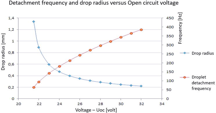
Figure 6 below shows the growth period and maximum droplet radius size along with the detachment frequency for each stress value.

Figure 6.

Droplet detachment frequency and size with open-circuit voltage variations.

The drop is ranging from (½ re) to (1 re +2 rg). With these relations, it is possible to describe the solid wire and cast wire equation and correlate them with the following equations (Eqs. (22) and (23)):

$$\mathrm{la}=15–\mathrm{ls}–\mathrm{lac}$$E22

$$\mathrm{Cs}=\mathrm{ls}+\mathrm{lac}–\mathrm{Cl}$$E23

Where Cl is the length of cast wire.

To model the detachment of the drop, the application of the Fourier series was proposed for a saw-type wave, and using the first 4 terms of sine, together with the equations described above for the period and volume of the drop, Eq. (24) below to model droplet size variation and cast wire length (Cl). Where:

$$\begin{array}{ll}\mathit{Cl}=& \left(\raisebox{1ex}{$1$}\!\left/ \!\raisebox{-1ex}{$2$}\right.r_e+2r_g\right)\ast [\frac{1}{\pi }\ast [\mathit{sen}\left(x-\frac{\pi }{2}\right)-\frac{1}{2}\mathit{sen}\left(2x-\frac{\pi }{2}\right)+\frac{1}{3}\mathit{sen}\left(3x-\frac{\pi }{2}\right)\\ & -\frac{1}{4}\mathit{sen}\left(4x-\frac{\pi }{2}\right)]+1+\frac{1}{2}{r}_e]\end{array}$$E24

Because: X = W*t, and X is cyclic, then X = 2Π/Δt. Substituting $r_e$, $r_g$, X and Δt in the equation we get (Eq. (25)):

$$\begin{array}{ll}\mathit{Cl}=& \left(0.3+\frac{3}{2}\ast \mathit{Ws}\ast \frac{10,5}{{\left(\mathit{Uoc}-21\right)}^{7/12}}\right)\ast \frac{1}{\pi }\ast [\mathit{sen}\left(\frac{2\pi {\left(\mathit{Uoc}-21\right)}^{7/12}}{10,5}-\frac{\pi }{2}\right)\\ & -\frac{1}{2}\mathit{sen}\left(\frac{4\pi {\left(\mathit{Uoc}-21\right)}^{7/12}}{10.5}-\frac{\pi }{2}\right)+\frac{1}{3}\mathit{sen}\left(\frac{6\pi {\left(\mathit{Uoc}-21\right)}^{7/12}}{10.5}-\frac{\pi }{2}\right)\\ & -\frac{1}{4}\mathit{sen}\left(\frac{8\pi {\left(\mathit{Uoc}-21\right)}^{7/12}}{10.5}-\frac{\pi }{2}\right)+1+\frac{1}{2}\ast r_e]\end{array}$$E25

To facilitate the handling of this equation (Eq. (25)) in the state model, it will be placed from now on as:

$$\mathit{Cl}=\left(0.3+\frac{3}{2}\ast \mathit{Ws}\ast \frac{10,5}{{\left(\mathit{Uoc}-21\right)}^{7/12}}\right)\ast \frac{1}{\pi }\ast \left[\ast \ast \ast \right]$$E26

Where the expression [***] is the Fourier expression belonging to the sines.

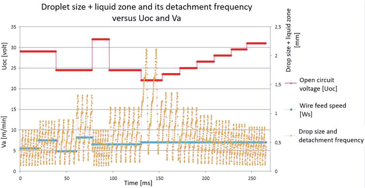
Using training values with input variables such as source output voltage (Uoc) and wire feed speed Ws, one obtains the drop size value and detachment frequency shown in Figure 7 below.

Figure 7.

Different Cl sizes and detachment frequencies simulated for open-circuit voltage variations.

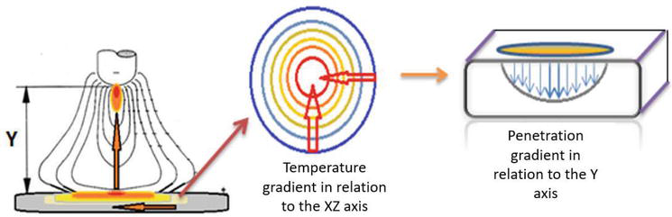
Performing an analysis of the shape of the plasma in the captured images, where a source of direct current with reverse polarity was used, it presented a bell shape, as expected according to the references. The energy released in the displacement of electrons is given by E = I*V*Δt, the voltage drops define areas where there is more consumption of this energy. Part is dissipated in cables and connections, but most is being consumed in cathode, anode, and plasma. This energy can be visualized by the isotherms, in Figure 8.

Figure 8.

Scheme of isotherms and temperature gradients and the relationship with the penetration gradient.

The isotherms show temperature gradients from the plate to the tip of the wire in the Y axis and from the outside to the center of the arc in the XZ direction radially around a circle. The T° gradient in the XZ and Y isotherms close to the part has a relationship with the gradient in penetration. We first analyze the relationship between the width and the energy contained in the plasma volume to propose an equation for the state-space model. There is a total energy of the system and an energy consumed in the plasma expressed in the following equations (Eqs. (27) and (28)):

$$\mathit{Et}=I\ast V\ast \mathit{dt}$$E27

$$\mathit{Ep}=C8\ast V_{\mathit{pl}}\ast \mathit{dt}$$E28

Where Vpl is the plasma volume approximated to the volume of a cone and with some other considerations one arrives that the plasma volume equation is (Eq. (29)):

$$\mathit{Vpl}=\frac{1}{12}\ast \pi \ast {\mathit{La}}^2\ast \left(l_a+r_e\right)$$E29

Therefore (Eq. (30)):

$$I\ast V=C8\ast \frac{1}{12}\ast \pi \ast {\mathit{La}}^2\ast \left(l_a+r_e\right)$$E30

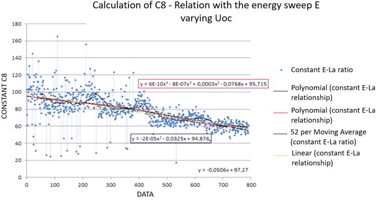
Where La is the bead width and la is the arc length. Isolating C8 and replacing the values of I, V, La, and $l_a$ by experimental values in droplet mode, we obtain the value of C8. The result shows a trend, but due to the dispersion of the data, a linear and polynomial approximation of degree 2 is performed. The tendency of C8 to decrease with the proportional increase of Uoc every 200 data points is shown in Figure 9. It is also observed how the dispersion of the values is smaller with higher voltages, indicating greater stability of the system when increasing the voltage.

Figure 9.

Calculation of equations that model the variation of C8 with the variation of power or consumed energy.

Using an additional linear relationship in the equation in the work range for dropleting and with experimental values, the constant C8 = 90 was found and isolating La we obtain (Eqs. (31) and (32)):

$${\mathit{La}}^2=\frac{12\ast I\ast \mathit{Uoc}}{\pi \ast \left(l_a+r_e\right)\ast \left(90-\left(\mathit{Uoc}-26,5\right)\ast 10\right)}$$E31

$$\mathit{La}=\sqrt{\frac{12\ast I\ast \mathit{Uoc}}{\pi \ast \left(l_a+r_e\right)\ast \left(90-\left(\mathit{Uoc}-26,5\right)\ast 10\right)}}$$E32

Where to CTWD = 15 if have: $l_a$ = 15 – $l_s$ and $l_s$ = X1.

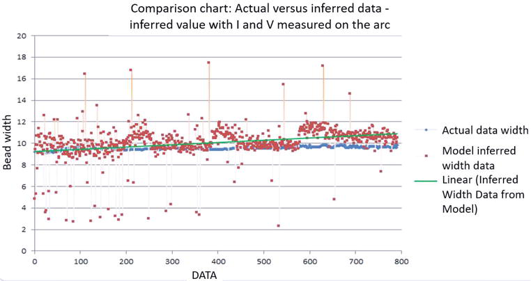
Was used experimental data to test the proposed equation (Eq. (32)). Where current and voltage in the arc are noisy because of droplet formation and detachment as well as changes in conduction zone and arc length mentioned earlier. The proposed equation, even with this noise, shows a tendency in the prediction of the width as shown in Figure 10. But using all the equations of state with adjustments and without using the experimental current values, the prediction improves a lot.

Figure 10.

Previous test of the width prediction values of the X6 equation of state, using experimental data of voltage and current in the arc at the transition point and comparing with the actual width data.

Substituting the notation of the variables to use in the state model, we get (Eqs. (33) and (34)):

$$X6={\left(\frac{12\ast U1}{\pi \ast \left(90-\left(U1-26,5\right)\ast 10\right)}\right)}^{\raisebox{1ex}{$1$}\!\left/ \!\raisebox{-1ex}{$2$}\right.}{\left(\frac{X2}{\left(15-X1+r_e\right)}\right)}^{\raisebox{1ex}{$1$}\!\left/ \!\raisebox{-1ex}{$2$}\right.}$$E33

$$\dot{X6}={\left(\frac{12\ast U1}{\pi \ast \left(90-\left(\mathit{Uoc}-26,5\right)\ast 10\right)}\right)}^{\raisebox{1ex}{$1$}\!\left/ \!\raisebox{-1ex}{$2$}\right.}\ast \frac{1}{2}{\left(\frac{X2}{\left(15-X1+r_e\right)}\right)}^{\raisebox{1ex}{$-1$}\!\left/ \!\raisebox{-1ex}{$2$}\right.}\ast \frac{\dot{X2}\ast \left(15-X1+r_e\right)-\dot{X1}\ast X2}{{\left(15-X1+r_e\right)}^2}$$E34

The other equation of state to determine the value of reinforcement and the relation with the width comes from the relation of volumes, the molten volume of the wire (Vfr) and the deposited volume (Vd) which depends on the welding speed and the cross section of the cord per unit time. These volume expressions are expressed below (Eqs. (35) and (36)):

$$\mathit{Vf}=A1\ast \mathit{Ws}\ast \mathit{dt}=A1\ast \mathit{Ws}\ast ∆t$$E35

$$\mathit{Vd}=\mathit{Vf}=A2\ast \mathit{Ts}\ast \mathit{dt}=A2\ast \mathit{Ts}\ast ∆t$$E36

Equating the equations (Eq. (37)):

$$A1\ast \mathit{Ws}=A2\ast \mathit{Ts}$$E37

Where:

$A1=\pi \ast {r_e}^2$;

$A2=\pi \ast \frac{a\ast b}{2}$;

$a=R$;

$b=\mathit{La}/2$;

Replacing and isolating the reinforcement R (Eq. (38)):

$$R=\frac{4\ast {r_e}^2\ast \mathit{Ws}}{\mathit{La}\ast \mathit{Ts}}$$E38

Substituting the reinforcement equation for the state variables, we have (Eq. (39)):

$$X7=\frac{4\ast {r_e}^2\ast X3}{X6\ast X5}$$E39

The last proposed equation of state is the relationship between penetration and other variables, which will depend on constants specific to the material, such as material density, thermal conduction, specific heat, enthalpy of fusion, electrical conductivity, electrical resistance, thermal energy, arc voltage drop, anodic voltage drop, thermal dissipation by conduction, convection and radiation, exposure time of the arc with the puddle which will depend on the welding speed, and area of contact of the plasma with the piece which will depend on the length of arc and this in turn of the wire speed and the tension. Due to the large number of variables, it was decided to simplify the equation and leave the variables with the greatest influence on penetration. After analyzing the energy required to melt the metal pool, and the energy in the plasma created by the current, the following equation is proposed (Eq. (40)):

$$P=\left(\frac{\mathit{Cf}\ast C5\ast I\ast \mathit{Ua}}{\rho \ast \pi \ast {\left(\frac{\mathit{La}}{2}\right)}^2\ast \mathit{Ts}}\right)$$E40

Leaving only one constant $C9=\left(\frac{4\ast \mathit{Cf}\ast C5\ast C6}{\rho \ast \pi }\right)$; replacing is (Eq. (41)):

$$P=C9\ast \left(\frac{I\ast \mathit{Uoc}}{{\mathit{La}}^2\ast \mathit{Ts}}\right)$$E41

Substituting for the state variables, we get (Eq. (42)):

$$X8=C9\ast \left(\frac{X2\ast U1}{X{6}^2\ast X5}\right)$$E42

Finally, replacing lac and Cl in Eq. (22) we get Eq. (42) for Cs (Eq. (43)).

$$\mathit{Cs}=\mathit{ls}+\frac{\left(e^{0.38\ast {\left(\mathit{Uoc}-23\right)}^{\frac{1}{3}}}-0.032\ast {l_a}^{\frac{3}{2}}-0.42\right)}{\pi \ast {r_e}^2}-$$

$$\left(0.3+\frac{3}{2}\ast \mathit{Ws}\ast \frac{10,5}{{\left(\mathit{Uoc}-21\right)}^{7/12}}\right)\ast \frac{1}{\pi }\ast \left[\ast \ast \ast \right]$$E43

Substituting for the state variables and knowing that la = 15 –X1, we have (Eq. (44)):

$$\mathit{Cs}=X1+\frac{\left(e^{0.38\ast {\left(\mathit{Uoc}-23\right)}^{\frac{1}{3}}}-0.032\ast {\left(15-\mathrm{X}1\right)}^{\frac{3}{2}}-0.42\right)}{\pi \ast {r_e}^2}-$$

$$\left(0.3+\frac{3}{2}\ast X3\ast \frac{10,5}{{\left(\mathit{Uoc}-21\right)}^{7/12}}\right)\ast \frac{1}{\pi }\ast \left[\ast \ast \ast \right]$$E44

Below is Table 4 with the constants used for the parameterization of the proposed model.

Nomenclature	Symbol	Value (unit)
Total resistance	Rs	6.8 * 10^−3 (Ω)
Total inductance	Ls	306*10^−6 (H)
Arc resistance	Ra	0.0237 (Ω)
Arc length voltage factor	Ea	400 (V.m^−1)
Electrode resistance	ɤe	0.43 (Ω.m^−1)
Space permeability	Pe	1.257 * 10^−6 (Kg.m.s^−2A^−2)
Gravity	G	9.8 (m. s^−2)
Liquid electrode density	${\rho }_e$	7800 (Kg.m^−3)
electrode radio	re	0.0012 (m)
Plasma Density	${\rho }_p$	1.6 (Kg.m^−3)2)
Time constant of wire and table motors	τm	50*10^−3 (s)
engine profit	Km	1.0 (mV^−1 s^−1)
Surface tension of the material	γ	1.3 (N.m^−1)

Table 4.

Constants used for the parameterization of the proposed model.

Other constants used in the state-space model such as C1 and C2 are multiplications of inductances, resistances, and constant coefficients that are repeated in the equations. The model needs parameterization, for a more accurate prediction, but the model also contributes to a better understanding of the behavior of the system or plant. Next, write the projected equations for each state, with the simplifications (Eqs. (45)–(52)):

$$\dot{X1}=X3-\left(\frac{C1}{\mathrm{\Pi }{\mathit{re}}^2}X2+\frac{C2}{\mathrm{\Pi }{\mathit{re}}^2}X1.X{2}^2\right)$$E45

$$\dot{X2}=\frac{1}{\ell \mathrm{s}}\left[U1-\left\{\mathit{Rs}+r\left(\ell \mathrm{s}+\frac{1}{2}.{\left(\frac{3\mathit{md}}{4\mathrm{\Pi }\mathit{re}}\right)}^{\frac{1}{3}}+\mathit{Xd}\right)+\mathit{Ra}\right\}.X2-\mathit{Ea}\left(\mathit{lc}-X1\right)-\mathit{Uo}\right]\left(\ast \right)$$E46

$$\dot{X3}=\frac{1}{\mathit{Tma}}\left(\mathit{\text{KmaU}}2-X3\right)$$E47

$$\begin{array}{ll}\dot{X4}=& X1+\frac{\left(e^{0.38\ast {\left(U1-23\right)}^{\frac{1}{3}}}-0.032\ast {\left(15-\mathrm{X}1\right)}^{\frac{3}{2}}-0.42\right)}{\pi \ast {r_e}^2}\\ & -\left(0.3+\frac{3}{2}\ast X3\ast \frac{10.5}{{\left(\mathit{Uoc}-21\right)}^{7/12}}\right)\ast \frac{1}{\pi }\ast \left[\ast \ast \ast \right]\end{array}$$E48

$$\dot{X5}=\frac{1}{\mathit{Tms}}\left(\mathit{\text{KmsU}}3-X5\right)$$E49

$$\dot{X6}={\left(\frac{12\ast U1}{\pi \ast \left(90-\left(U1-26,5\right)\ast 10\right)}\right)}^{\raisebox{1ex}{$1$}\!\left/ \!\raisebox{-1ex}{$2$}\right.}\ast \frac{1}{2}{\left(\frac{X2}{\left(15-X1+r_e\right)}\right)}^{\raisebox{1ex}{$-1$}\!\left/ \!\raisebox{-1ex}{$2$}\right.}\ast \frac{\dot{X2}\ast \left(15-X1+r_e\right)-\dot{X1}\ast X2}{{\left(15-X1+r_e\right)}^2}$$E50

$$\stackrel{̇}{\dot{X7}=\frac{4\ast {r_e}^2\frac{1}{\mathit{Tma}}\left(\mathit{\text{KmaU}}2-X3\right)\ast X6\ast X4-4\ast {r_e}^2\ast X3\ast \left(X6\ast \frac{1}{\mathit{Tms}}\left(\mathit{\text{KmsU}}3-X4\right)+\dot{\left(""\right)}\ast X4\right)}{X{6}^2\ast X{4}^2}}$$E51

Where (“”) is Eq. state 6 to $\dot{X6}$

$$\dot{X8}=C9\ast \left(\frac{U1\ast \dot{X2}\ast X{6}^4\ast X{5}^2-U1\ast X2\ast \left(X{6}^2\ast \dot{X5}+2X6\ast X5\right)}{X{6}^4\ast X{5}^2}\right)$$E52

3. Conclusion

This work had the proposal to develop a mathematical model by equation of states, a dynamic model that can generalize to the globular and droplet ranges and predict the proposed outputs, width, reinforcement and penetration, through input values for the state variables used to control. The use of real data (shadowgraph, infrared camera, high-speed camera) for model calibration allows guaranteeing the reliability of the predicted results when using the state equations.

Acknowledgments

To CAPES for the financial support and to the University of Brasilia for the necessary infrastructure to carry out the tests.

Conflict of interest

The authors declare no conflict of interest.