Blown Film Cooling Numerical and Experimental Investigations

Abstract

The blown film production process involves several processes as extrusion and film cooling. The demand to achieve high productivity with proper film quality has devoted the researchers to investigating in detail, the bubble kinematics, and the thin film cooling process, utilizing the powerful Computational Fluid Dynamics tools, which allows them to deeply study the flow field, and the related heat transfer from the hot thin film to the surrounding mediums, several runs can be done, resulting in huge scientific data, at a minimum cost. In addition to the experimental measurements. The combination of both, reveals better understanding and accurate results.

1. Introduction

Blown film production is a widely used polymer processing technology that has been developed considerably during the past decades. The increasing demand to achieve high productivity with high-quality film products has steered more researchers to devote their efforts towards the investigation and development of both equipment and materials used in the blown film industry [1, 2, 3, 4, 5, 6, 7].

Blown film production involves several complex processes as the following: -

• Extrusion

  During the blown film production process, the polymer pellets are poured inside the hopper and then forced by the screw to flow inside the extruder’s barrel. Where the polymer pellets are heated and melted into a viscous fluid, flowing between the extruder’s barrel and the rotating screw. The heat conducted from the electric strip heaters through the barrel walls and into the polymer, in addition to the viscous dissipation due to the screw rotation, melts the polymer. The heating process depends on the thermo-physical properties of the polymer under processing, such as High-Density Polyethylene (HDPE), Low-Density Polyethylene (LDPE), etc. The melt exits from a circular orifice at the top of the die forming a bubble. Pressurized air is introduced into the center of the die to inflate the bubble to take the desired dimensions. The bubble radius and thickness variations along the machine direction are controlled by several operating parameters like the polymer being processed, the size of both the die and the cooling air ring, the internal air pressure, the cooling airflow rate, the melt throughput and the take-off speed, which is defined as the velocity of the blown film as it travels through the nip rollers. Figure 1 shows a typical blown film production system.

• Film cooling

  The cooling process helps the polymer to cool down after it takes the desired shape, dimensions, and final characteristics. Mainly, there are two common air-cooling techniques used in the blown film production process.

  • The internal bubble cooling (IBC)

    Where pressurized air is introduced into the center of the die, circulated inside the bubble to cool down the internal bubble surface, and then exhausted outside through the die. This internal cooling air is also used to inflate the bubble.

  • The external bubble cooling (EBC)

    The outer surface of the bubble is cooled via an air ring, which is fed from the air blower through several inlet ports distributed on either its side or bottom walls. The air rings are usually designed to be adjustable to control the cooling airflow rate, which exits through the gap between its lips. Air rings would have either single or multiple lips according to the characteristics of the polymer being processed. The air ring has to be aligned correctly with the bubble to guarantee equal distribution of the cooling air around the bubble’s body which in turn reduces the possibility to get thickness variation on the bubble lay-flat.

    One typical air ring design is the single-lip type, which is relatively inexpensive. This design is used with polymer materials that are run with stable bubbles, such as HDPE with a low Melt Index (MI) < 0.1, which is characterized by its long stalk. The MI is defined as the mass of polymer, in grams, flowing in ten minutes through a capillary of a specific length and diameter by applying pressure via prescribed alternative gravimetric weights for alternative prescribed temperatures [8]. While the dual-lip air ring is used with less stable polymer materials that are run with a pocket bubble type. Figure 2 shows the two air ring designs.

• Film collapsing

  The film tube passes through the nip rolls where it is collapsed and flattened. The material of the nip rolls has to have low thermal conductivity to avoid film surface defects. Then the film is wrapped into rolls. The film winder has to be aligned well with the upstream equipment to avoid applying undesirable stresses on the film layers.

• Production control

  The blown film production machine shall be equipped with film thickness control and monitoring devices, which measure and correct the thickness variations along the bubble’s circumference at the Frost-Line Height (FLH). Besides, bubble stability monitoring and control devices are used to guarantee a stable production process with proper high-quality blown film products.

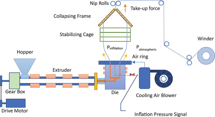
Figure 1.

Typical blown film production system.

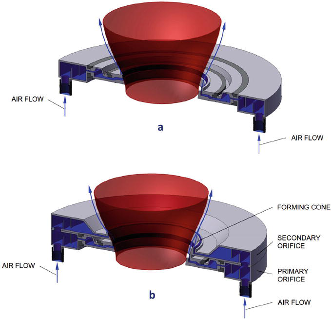
Figure 2.

Typical cross-sections of both single and dual-lip air rings: (a) the single-lip design, (b) the dual-lip design.

2. Blown film materials

For blown film products, the desired properties determine the fit for the purpose material needed for a specified application. Blown film extrusion requires good processing characteristics in addition to high-quality products. The most important properties of blown film products are:

• Optical properties, such as optical thickness, transmissivity to thermal radiation and haziness.

• Mechanical properties, like tensile strength and tear resistance.

• Thermal properties, such as solidus and liquidus temperatures, the viscosity of the melt phase, the thermal conductivity, etc.

The ease of the blown film production process can be defined by several material characteristics such as good thermal stability, high melt strength downstream of the die exit, proper head pressures, and film surface clarity. Finally, cost optimization is a key factor.

Polyethylene (PE) is considered the best polymer for most blown film production applications. It has good water resistance, is lightweight, has an acceptable balance of flexibility and strength, and can have good clarity. Moreover, PE is considered easy to heat-seal and extrude, at a low cost. In addition to the above-mentioned common properties of PE, it is a polymer that is well understood scientifically, this led to well-designed and controlled polymerization techniques to yield specific property values over a very wide range. Particularly, PE grades can be produced with better clarity, acceptable higher strength than average, more flexibility, etc. Within the broad family of polyethylene, different types are used in the blown film extrusion industry as follows:

2.1 Polyethylene (PE)

Based on a chemical point of view, it is considered the simplest polymer. PE is polymerized from an ethylene monomer, which contains a carbon chain backbone with two hydrogen atoms bonded to each carbon atom. Individual chains or molecules would contain tens to hundreds of carbon atoms. Chains can be branched or linear, based on how the polymer was synthesized. There are several synthesizing techniques for polyethylene production [9]. All PE grades are characterized by high specific heat values, which means a relatively slow heat removal from the polymer during processing. The specific heat of PE is about 2 kJ/kg·K compared to approximately 1 kJ/kg·K for most other different polymers. Consequently, cooling towers for PE-blown film production are extremely tall. It requires enough time to release the remaining heat from the two layers of the film moving through the nip rollers to prevent them from blocking.

2.2 Low-density polyethylene (LDPE)

Polyethylene is often classified according to its density. When a polymer cools from the melt state and solidifies, some of the chains would organize into denser, highly ordered crystalline zones. LDPE has a density that varies between 0.93 and 0.91 g/cm³. It has good processing characteristics and does not require too much motor torque to rotate the screw. Besides, it melts at approximately 105–115°C. On the other hand, the existence of a wide range of branching yields a bubble with high melt strength and an adequately wide processing window. The LDPE films possess a good combination between elongation and strength in addition to good flexibility.

2.3 High-density polyethylene (HDPE)

Is synthesized by a different method that is used for LDPE. It is produced with linear chains. HDPE is polymerized with a few amounts of comonomer and results in a few short-chain branches. Which are placed intentionally along the main chain to get a polymer with good processability. A high degree of linearity produces a polymer with a high percentage of crystallinity and consequently high density. HDPE has a density range of 0.96–0.93 g/cm³. HDPE melts at relatively higher temperatures 130–135°C. Furthermore, it has a narrower processing window. In addition, it consumes a high screw torque.

One of the clearest differences between processing HDPE and LDPE is that, HDPE with a low MI< 0.1 runs usually with a high FLH. Which is about 8–10 times the bubble’s initial diameter at the die. Bubble instabilities would exist during the processing of HDPE due to its lower melt strength. Delaying bubble transverse stretching until the melt gets cooler i.e., at higher FLH, the bubble becomes more stable. In addition, HDPE-blown films are characterized by their high stiffness and strength. Hence, there is persistent progress to produce HDPE film products with small thicknesses.

2.4 Linear low-density polyethylene (LLDPE)

LLDPE is considered a variation of HDPE. It is manufactured in the same way with many comonomers, such as octane or hexene. The existence of a comonomer in the chain results in shorter-chain branches of a certain length. The density of LLDPE varies between 0.93 and 0.88 g/cm³ and has a melt temperature of 115–125°C. Processing of LLDPE needs high screw torque with a grooved feed throat similar to HDPE. However, outside of the die, it is processed with a pocket bubble profile similar to LDPE, even though the melt strength is lower than that of LDPE. To guarantee proper bubble stability, dual or multiple-lip air rings are used for high cooling airflow rates. The LLDPE film’s final properties are considered a combination of those of LDPE and HDPE.

3. Machine setup requirements

The setup of the blown film production machine requires the adjustment of the following operating parameters, which shall be performed by skilled technicians.

• The temperature of the heaters according to the specified melting temperature of the polymer being processed like HDPE, LDPE, LLDPE, etc.

• The inflation pressure shall be higher than the atmospheric pressure.

• The inflation air volume has to be adjusted with the inflation pressure to get the desired bubble’s profile and characteristics:

  • The Blow-Up ratio (BUR), is the ratio of the bubble’s diameter at the FLH to that at the die exit.

  • The FLH is the height at which, the bubble’s radius and the film thickness become fixed. Moreover, it corresponds to the optimum cooling and desired film properties.

• The Take-Up Ratio (TUR) is defined as the ratio between the film velocities at the FLH to that at the die exit.

The final film dimensions and characteristics are obtained by performing fine-tuning between the above-mentioned parameters.

4. Numerical and experimental investigations

During the blown film production process, the molten polymer exits the die through a circular orifice at its top, forming a bubble with varying radius and thickness. The bubble body is subjected to the differential pressure between the internal inflation pressure, and the external atmospheric pressure, the take-up force which pulls the film up in the machine direction, see Figure 1, and the cooling air which cools down the hot bubble and transforms it to the solid phase after taking the desired dimensions and characteristics. The complex processes associated with the production of the blown film reveal different related research fields, which can be categorized as follows:

• Rheology, where the bubble kinematics are mainly considered [1, 10, 11]. The bubble’s profile and the film thickness variation along the machine direction are investigated numerically and experimentally for different polymer viscosity modeling and different operating conditions.

• Aerodynamics of the blown film cooling, where the flow field around the bubble’s surfaces and the corresponding heat transfer are investigated. In addition to, the air ring design and its influence on the generated flow field and the cooling efficiency [5, 7, 12, 13, 14].

• Experimental measurements are applied to investigate the bubble’s profile, the surface temperature, and the film thickness variations with the machine direction, the film’s mechanical and optical properties, and the bubble’s stability monitoring and control [2, 15].

• Recently, due to the progress that occurred in the field of blown film production, the dependency of the bubble kinematics on the film surface temperature distribution and the temperature gradients inside the film thickness, some researchers devoted their efforts to combining the blown film aerodynamics with the bubble kinematics [6, 16, 17, 18, 19]. Besides, the bubble’s stability during the production process is also investigated as an important monitoring issue [20].

5. Numerical modeling guidelines

The use of Computational Fluid Dynamics (CFD) as a simulation tool enables the researchers to study in detail the physical phenomena associated with the flow pattern and the related heat transfer process. Besides, several runs and design optimizations can be done in a short time and at a minimum cost. The calculation domain in blown film cooling can be divided into three distinct zones namely, the external cooling air domain, the bubble body domain, and the internal air\cooling air domain as illustrated in Figure 3.

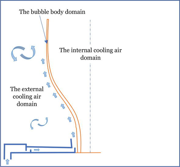
Figure 3.

Blown film cooling calculation domains.

5.1 The turbulent cooling airflow numerical modeling

Blown film cooling airflow is mostly turbulent. The selection of the more accurate turbulence model, the required near-wall treatments, in addition to the mesh size requirements while constructing the calculation domain matters. The turbulence modeling passed several modifications during the past decades, the basis of the first step was the time averaging of the governing equations.

5.1.1 The Reynolds Averaged Navier Stokes (RANS) Equations

Starting with the incompressible, constant-property flow. The conservation equations of mass and momentum take the following forms:

$$\frac{\partial u_i}{\partial x_i}=0$$E1

$$\rho \frac{{\partial u}_i}{\partial t}+\rho u_j\frac{{\partial u}_i}{\partial x_j}=-\frac{\partial p}{\partial x_i}+\frac{{\partial t}_{\mathit{ji}}}{\partial x_j}$$E2

The vectors $x_i$ and $u_i$, are position and velocity, t is time, p is static pressure, ρ is density and $t_{\mathit{ij}}$ is the viscous stress tensor defined by

$$t_{\mathit{ij}}=2\mu s_{\mathit{ij}}$$E3

Where the strain-rate tensor is defined by:

$$s_{\mathit{ij}}=\frac{1}{2}\left(\frac{\partial u_i}{\partial x_j}+\frac{\partial u_j}{\partial x_i}\right)$$E4

Applying time averaging on Eqs. (1) and (2), yields the well-known Reynolds Average Equations of motion in its conservation form, viz.

$$\frac{\partial U_i}{\partial x_i}=0$$E5

$$\rho \frac{{\partial U}_i}{\partial t}+\rho U_j\frac{\partial U_i}{\partial x_j}=\frac{-\partial P}{\partial x_i}+\frac{\partial }{\partial x_j}\left(2{\mathit{\mu S}}_{\mathit{ji}}-\rho \overline{u_i^{\prime }{u}_j^{\prime }}\right)$$E6

The only difference between the instantaneous and the time-average momentum equations is the existence of the correlation $\overline{u_i^{\prime }{u}_j^{\prime }}$ , which is the time-average rate of momentum transfer because of turbulence. Moreover, the quantity $-\mathit{\rho }\overline{{\mathit{u}}_i^{\prime }{u}_j^{\prime }}$ is the Reynolds-stress tensor. The computation of this term is the fundamental problem of turbulence modeling. The RANS models can be closed as follows:

5.1.2 The Reynolds-Stress Model (RSM)

In this model, the specific Reynolds stress tensor is directly solved via transport equations. However, modeling is still needed for several terms in the transport equations. The RSM is more advantageous in complex three-dimensional turbulent flows possessing swirl and large streamline curvature. The RSM model is more complicated to converge than eddy viscosity models. Besides, it is computationally intensive.

5.1.3 The Eddy Viscosity Models, (Boussinesq hypothesis)

The Reynolds stresses are modeled by introducing turbulent or eddy viscosity,${\nu }_T$.

$${\tau }_{\mathit{ij}}={\nu }_T\left(\frac{\partial \overline{u_i}}{\partial x_j}+\frac{\partial \overline{u_j}}{\partial x_i}\right)-\frac{2}{3}k{\delta }_{\mathit{ij}}$$E7

Where the Kronecker delta function takes the form:

$${\delta }_{\mathit{ij}}=\left\{\begin{array}{c}1,i=j\\ 0,i\ne j\end{array}\right.$$E8

The Boussinesq hypothesis is suitable for simple turbulent shear flows such as boundary layers, round jets, channel flows and mixing layers, etc.

Noting that all turbulence models have empiricism because.

• Equations cannot be closed based on fundamental principles.

• Calibration is required to set up the model constants.

Based on the Boussinesq hypothesis, the dimensions of the turbulent kinematic viscosity ${\mathrm{\nu }}_{\mathrm{T}}$ is (length²/time) i.e., according to dimensional analysis, it can be considered as the product of velocity scale by a length scale.

Mainly there are four categories of eddy viscosity models:

• Algebraic or zero-equation models.

• One-equation models.

• Two-equation models.

• Stress-transport models.

We will move forward to the two-equation models.

5.1.3.1 Two-equation models

The improvement in computer capabilities since the 1960s allowed looking forward to utilizing more complicated models. For example, the turbulence models based on the equation formulating the turbulence kinetic energy have become the basis of modern research in turbulence modeling. The two-equation models are eddy-viscosity-based. That they retain the Boussinesq eddy-viscosity approximation.

Prandtl (1945) defined the turbulence kinetic energy (per unit mass) of turbulent fluctuations.

The specific turbulence kinetic energy, k is given by:

$$k=-\frac{1}{2}{\tau }_{\mathit{ii}}=\frac{1}{2}\overline{u_i^{\prime }{u}_i^{\prime }}=\frac{1}{2}\left(\overline{u^{\prime 2}}+\overline{v^{\prime 2}}+\overline{w^{\prime 2}}\right)$$E9

Based on the dimensional arguments, the kinematic eddy viscosity can be written as a product of a velocity scale by a length scale.

$${\nu }_T=C{k}^{1/2}\ell$$E10

Where C is a constant.

The transport equation for the turbulence kinetic energy k takes the following form:

$$\frac{\partial k}{\partial t}+U_j\frac{\partial k}{\partial x_j}={\tau }_{\mathit{ij}}\frac{\partial U_i}{\partial x_j}-\epsilon +\frac{\partial }{\partial x_j}\left[\nu \frac{\partial k}{\partial x_j}-\frac{1}{2}\overline{u_i^{\prime }{u}_i^{\prime }{u}_j^{\prime }}-\frac{1}{\rho }\overline{p^{\prime }{u}_j^{\prime }}\right]$$E11

The quantity $\epsilon$ is the dissipation rate per unit mass and is defined by:

$$\epsilon =\nu \overline{\frac{\partial u_i^{\prime }}{\partial x_k}\frac{\partial u_i^{\prime }}{\partial x_k}}$$E12

At this point, there are two unknowns, which are the turbulent length scale, $\ell$ and the dissipation rate,$\epsilon$. Both properties are assumed solely functions of turbulence only. The dimensional arguments of [Taylor (1935)] showed that:

$$\epsilon \sim k^{3/2}/\ell$$E13

The system of equations still needs a prescription for the turbulence length scale to be closed. Hence, the following version of the turbulence kinetic energy equation is applied in all turbulence energy equation-based models and takes the following simplified form:

$$\frac{\partial k}{\partial t}+U_j\frac{\partial k}{\partial x_j}=-{\tau }_{\mathit{ij}}\frac{\partial U_i}{\partial x_j}-\epsilon +\frac{\partial }{\partial x_j}\left[\left(\nu +{\nu }_T/{\sigma }_k\right)\frac{\partial k}{\partial x_j}\right]$$E14

Where ${\sigma }_k$ is a closure coefficient.

Moreover, Prandtl (1945) introduced a closure coefficient to Eq. (13) called$C_D$

$$\epsilon =C_D{k}^{3/2}/\ell$$E15

In any two-equation model, a second transport equation is needed to close the system.

The different two-equation-based models can be summarized as follows:

5.1.3.2 The $k-\omega$ model

The specific dissipation rate ω, with dimensions of (1/time), is selected as the second variable to close the system of equations. The developers of the $k-\omega$ model after Kolmogorov added a production term like Wilcox [21], Kok [22], and Hellsten [23]. The updated version of the $k-\omega$ model improved predictions of Wilcox model [21], for strongly separated and free shear flows. The $k-\omega$ showed good accuracy in predicting free shear, wall-bounded and complicated separated flows when compared with experimental data.

5.1.3.3 The $\mathit{k}-\mathit{\epsilon }$ model

The $k-\epsilon$ model is one of the famous two-equation models. It was developed by several authors such as Launder and Sharma [24]. The formulation of the exact second transport equation started by taking the moment of the Navier-Stokes equation, and resulted in the well-known standard $k-\epsilon$ model [25]. Yakhot et al. [26] used techniques from the Renormalization Group (RNG) theory and developed the standard $k-\epsilon$ model to be the well-known RNG $k-\epsilon$ model. The new model uses a differential equation to calculate the turbulent viscosity, an analytical formula to calculate the turbulent Prandtl number and a modified new coefficient to improve the accuracy for rapidly strained flows.

5.1.3.4 The baseline (BSL) $\mathit{k}-\mathit{\omega }$ model

This model is formulated to combine the advantages of the$k-\epsilon$ model, which performs well for the outer wake region, and the $k-\omega$ model, which is more accurate for the inner zone of the boundary layer [27]. A blending function $F_1$is used and formulated to gradually change from one in the near-wall region to zero away from the walls. The BSL model is formulated by transforming the $k-\epsilon$ model into a $k-\omega$ model. Then, assuming ${\varsigma }_1$ represents any constant of the original$k-\omega$ model, ${\varsigma }_2$ any constant of the transformed $k-\epsilon$ model and $\mathrm{\varsigma }$ is any constant of the new BSL formulation. The baseline model retains the advantages of the $k-\omega$ model for wall-bounded flows without freestream dependency.

5.1.3.5 The shear stress transport (SST) $\mathit{k}-\mathit{\omega }$ model

The formulation of the $\mathrm{SST}k-\omega$ model is the same as the$\mathrm{BSL}k-\omega$, with a modified definition of the turbulent viscosity ${\nu }_T$ to control the overproduction of turbulent shear stress in adverse pressure gradient flows, a blending function $F_2$ is used [27]. The SST $k-\omega$ model has very good behaviour in separation flows and adverse pressure gradients. Nevertheless, it would produce a bit too large turbulence levels in regions with large normal strains, such as stagnation regions.

5.2 The energy equation

In addition to the previously described turbulence models, which are formulated to obtain the average velocity and pressure fields, the energy equation is solved to obtain the corresponding average temperature field.

The general form of the turbulent transport of the total energy E takes the following form:

$$\frac{\partial \left(\mathit{\rho E}\right)}{\partial t}+\frac{\partial \left(\rho U_{i}E\right)}{\partial x_i}=\frac{\partial }{\partial x_i}\left[\alpha {\mu }_{\mathit{eff}}{C}_p\frac{\partial T}{\partial x_i}+U_i{\left({\tau }_{\mathit{ij}}\right)}_{\mathit{eff}}\right]-\frac{\partial \left(P{U}_i\right)}{\partial x_i}$$E16

Where $\alpha$ is the inverse Prandtl number.

The polymer flow is simulated as a fluid moving through a virtual converging channel in the machine direction, where it is transformed from melt to solid phase due to the cooling process.

The energy equation for the polymer film takes the following form:

$$\frac{\partial \mathit{\rho H}}{\partial t}+\nabla .\left(\rho \overrightarrow{u}H\right)=\nabla .\left(K.\nabla T\right)+S$$E17

Where H is the material enthalpy $H=h+∆H$, $\overrightarrow{u}$ is the velocity vector, and S is a source term.

The thermal boundary condition at the film surface:

$$-K{\left.\frac{\partial T}{\partial n}\right|}_{\mathit{Fs}}=\left({\mathit{HTC}}_C+{\mathit{HTC}}_R\right)\left(T_{\mathit{Fs}}-T_{\infty }\right)$$E18

Further, near-wall treatments and turbulence kinetic energy production limiters are applied to improve the accuracy of the two-equation models [25, 28].

5.3 Blown film thermal radiation characteristics

Blown films’ thickness varies between a few millimeters at the die, to a few microns at the FLH, Figure 4 shows that thin polyethylene films are highly transparent to infrared thermal radiation except at 3.4 & 6.7 μm wavelengths, where their transmissivity is nearly dropped to zero. As illustrated, a 30 μm polyethylene film has a maximum of 90% transmissivity, and a 130 μm film is 70% [29]. According to Beer-Lambert’s law [30, 31], transmissivity takes the following form:

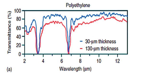
Figure 4.

Transmissivity versus wavelength for polyethylene film at 30 and 130 μm thicknesses [29].

$$\zeta \left(x\right)={\left(1-\varrho \right)}^2{e}^{-\mathit{\gamma n}\left(x\right)}$$E19

Polyethylene films are characterized by low reflectivity $\mathrm{\varrho }$ about 0.05 [32]. Consequently, the transmissivity$\zeta \left(x\right)$ would approximately correlate with the film thickness as follows:

$$\zeta \left(x\right)=0.9e^{-\mathit{\gamma n}\left(x\right)}$$E20

Where n: is the film thickness and$\gamma$ is the absorption coefficient, a typical value of 0.045 (Mils⁻¹) is found to be a reasonable correlation value. The term $\mathit{\gamma n}$ is defined as the optical thickness. Noting that (one Mil) equals (0.001 in).

The accurate numerical simulation requires a proper treatment of the radiation heat transfer from, into, and through the semitransparent film. The Discrete Ordinates (DO) radiation model [28], is used to include radiation heat transfer into consideration.

5.4 Discretization error analysis

CFD simulations with the implementation of advanced numerical modeling tools allow a better physical-based representation of actual complex flows. The uncertainty of the numerical simulations’ accuracy remains very important to ensure its strength. Even though, there is good agreement with the experimental results. The implementation of the Richardson extrapolation method [33, 34], and the Grid Convergence Index (GCI) methodology has been evaluated over many CFD cases. It permits a proper quantification of the uncertainty present in grid convergence [35, 36, 37].

6. Experimental measurements

The blown film production process involves several necessary measurements, the cooling air flow rate, the melt throughput, the ambient conditions, the air ring and the head walls temperatures, the bubble’s profile, and the film thickness and temperature variations along the machine direction. Moreover, some mechanical and optical properties are measured as, tensile strength, tear resistance, and haziness. Besides, the bubble’s stability is also monitored during the production process.

6.1 The inlet cooling airflow rate calculations

The air blower provides air into the air ring through uniformly distributed inlet ports. Two methods can be used to calculate the inlet cooling air flowrate:

• By measuring the velocity profile along the pipe’s radius and calculating the flow rate by integration.

• By using a measuring tube to have a fully developed flow, and measuring the maximum velocity at the centerline as per the following algorithm:

Recalling the Direct Numerical Simulation (DNS) results [38], the turbulent pipe flow exhibits a universal behavior. Where the mean streamwise velocity varies logarithmically with the normal distance to the wall.

The law of the wall takes the following form for turbulent pipe flows:

$$\frac{u\left(r\right)}{u_{\tau }}=\frac{1}{\kappa }\mathit{ln}\frac{u_{\tau }\left(R-r\right)}{\nu }+B$$E21

Where $\kappa \approx 0.41$, and $B\approx 5$ for smooth surfaces.

R: is the pipe radius, r: is the normal distance from the pipe centerline, and$u_{\tau }$: is the friction velocity,$u_{\tau }=\sqrt{\frac{{\tau }_w}{\rho }}$.

The pipe average velocity is calculated as follows [38]:

$$\overline{u}=\frac{Q}{A}=\frac{1}{\pi R^2}{\int }_0^R{u}_{\tau }\left(\frac{1}{\kappa }\mathit{ln}\frac{u_{\tau }\left(R-r\right)}{\nu }+B\right)2\mathit{\text{πrdr}}$$E22

$$\frac{\overline{u}}{u_{\tau }}\approx 2.44\mathit{ln}\frac{u_{\tau }R}{\nu }+1.34$$E23

The ratio between the “pipe’s average to maximum” air velocity can be formulated as:

$$\frac{\overline{u}}{u_0}\approx {\left(1+1.3\sqrt{f}\right)}^{-1}$$E24

Where $f$ is the friction factor, and $u_0$ is the centerline maximum velocity.

$$f=0.316{{\mathit{Re}}_D}^{-0.25},4000<{\mathit{Re}}_D<{10}^5$$E25

Where the Reynolds number is based on the pipe’s hydraulic diameter, D and the average velocity, $\overline{u}$ is defined as:

$${\mathit{Re}}_D=\frac{\overline{u}D}{\nu }$$E26

On the other hand, one of the most widely used temperature-measuring non-contact devices is the Infrared (IR) pyrometer [39, 40]. By identifying the spectral bands, radiation thermometers can be selected and used to measure both the surface and below-surface temperatures of plastic films which are characterized by their transparency to infrared radiation [29]. For an opaque surface with unknown emissivity, the device can be calibrated via thermocouples such as the K-type [41].

Regarding the bubble’s profile and film thickness variations with the machine direction, Liu et al. [42] performed experimental investigations on blown films of LDPE, LLDPE and HDPE materials. During the experiments, a video camera was used to measure the bubble’s shape and the film velocity, while a remote infrared sensing device measured the film surface temperature.

Combinations between experimental and numerical investigations have been studied by several authors as the following:

Zatloukal and Vlček [6] developed a model to describe bubble formation by applying variational principles. The basis of this model is that the bubble’s shape shall satisfy the minimum energy requirements. The proposed simple analytically resolvable equation with four physical parameters had been derived from the variational principles, successfully describing different bubble profiles, including the HDPE wineglass shape, taking the take-up force and the internal bubble pressure into consideration. The results were in good agreement with the experimental data. Also, Zatloukal and Kolarik [19] performed experiments on a 9-layer blown film to investigate how the cooling process affects the film surface temperature variation, the bubble’s shape and the product’s mechanical properties. The obtained experimental data followed by the theoretical analysis were used to evaluate three different convective heat transfer models. Both internal and external bubble cooling techniques were applied. It was found that only the Muslet & Kamal heat transfer model was correctly able to capture the physical characteristics of the heat transfer between the bubble and the cooling air, especially in the case of a very high FLH. Moreover, Ismail, ME [43] performed numerical and experimental investigations on the external cooling of an HDPE bubble with a new design of a counter flow air ring design. The performance of four different two-equation-based turbulence models is compared to the experimental results of the measured air velocity via a five-hole pitot tube.

6.2 Measurements uncertainty

No measurement done as a part of any scientific research, no matter how carefully we look, can be considered exact. The quantification of the uncertainty associated with the measurements is very important to identify the value of the measurand precisely [44].

7. Conclusions

Blown film cooling is a very important, and complicated process. The enhancement of the cooling efficiency would improve productivity and film quality via the following:

• Applying new cooling techniques.

• Proper understanding of the thermal characteristics of the film, turbulence models, and utilization of the powerful CDF tools. The accurate selection of the most advanced turbulence models, with the supporting discretization error analysis, matters.

• Accurate measurements, supported by the uncertainty analysis, support the scientific investigations and verify the numerical analysis.

Nomenclatures

A	Cross-sectional area, [m^2]
C, CD	Constants, [---]
CP	Specific heat at constant pressure, [J/kg.K]
D	Diameter, [m]
E	Total Energy, [J]
f	Darcy friction coefficient, [---]
F1	Blending function used in the BSL & SST $k-\omega$ models formulation, [---]
F2	Blending function used in the SST $k-\omega$ model formulation, [---]
h	Sensible enthalpy, [J]
H	Material enthalpy, [J]
HTC	Heat transfer coefficient, [W/m^2.K]
i,j	Unit vectors in x and y directions, [---]
$\mathit{k}$	Turbulence kinetic energy, [m^2/s^2]
K	Thermal conductivity, [W/m.K]
$\mathbf{\ell }$	Turbulence length scale, [m]
n	Unit vector normal to the film surface direction, [---]
n(x)	Film thickness in the machine direction, [m]
p	Instantaneous pressure, [Pa]
${\mathit{p}}^{\prime }$	Fluctuating static pressure, [Pa]
P	Average static pressure, [Pa]
Q	Volumetric flow rate, [m^3/s]
r	Radial distance, [m]
R	Radius, [m]
Re	Reynolds number, [---]
sij	Instantaneous strain-rate tensor, [1/s]
S	Shear rate, [1/s]
Sij	Mean strain-rate tensor, [1/s]
t	Time, [s]
T	Temperature, [K]
tij	Instantaneous viscous stress tensor, [Pa]
u,v	Instantaneous velocity component in the x and y directions, [m/s]
${\mathit{u}}_{\mathit{i}}$	Instantaneous velocity in tensor notation, [m/s]
u^'	Fluctuating velocity component in x-direction, [m/s]
${\mathit{u}}_{\mathit{i}}^{\prime }$	Fluctuating velocity in tensor notation, [m/s]
$\overline{\mathit{u}}$	Fully developed crossectional average air velocity inside the inlet flowrate measuring tube, [m/s]
${\mathit{u}}_{\mathit{\tau }}$	Friction velocity, [m/s]
${\mathit{u}}_{\mathbf{0}}$	Fully developed centerline air velocity inside the inlet flowrate measuring tube, [m/s]
u(r)	Radial air velocity inside the inlet flowrate measuring tube, [m/s]
U	Mean velocity component in the x-direction, [m/s]
${\mathit{U}}_{\mathit{i}}$	Mean velocity in tensor notation, [m/s]
v^’	Fluctuating velocity component in the y-direction, [m/s]
w^’	Fluctuating velocity component in the z-direction, [m/s]
${\mathit{x}}_{\mathit{i}}$	Position vector in vector notation, [---]
α	Inverse Prandtl number, [---]
$\mathit{\gamma }$	The blown film absorption coefficient, [m^−1]
${\mathit{\delta }}_{\mathit{ij}}$	Kronecker delta function, [---]
$\mathit{\epsilon }$	Dissipation rate, [m^2/s^3]
$\mathit{\varsigma }$	Represents any constant of the new BSL $k-\omega$ model, [---]
${\mathit{\varsigma }}_{\mathbf{1}}$	Represents any constant of the original$k-\omega$ model, [---]
${\mathit{\varsigma }}_{\mathbf{2}}$	Represents any constant of the transformed $k-\epsilon$ model, [---]
$\mathit{\zeta }\left(\mathit{x}\right)$	Transmissivity of the blown film, [---]
$\mathit{\kappa }$	Von Karaman constant, [---]
$\mathit{\nu }$	Kinematic viscosity, [m^2/s]
${\mathit{\nu }}_{\mathit{T}}$	Turbulence kinematic viscosity, [m^2/s]
$\mathit{\rho }$	Density, [kg/m^3]
$\mathit{\varrho }$	The reflectivity of the blown film surface, [---]
μ	Molecular viscosity, [Pa.s]
${\mathit{\sigma }}_{\mathit{k}}$	Closure coefficient, [---]
${\mathit{\tau }}_{\mathit{ij}}$	Specific Reynolds stress tensor, [m^2/s^2]
${\mathit{\tau }}_{\mathit{w}}$	Surface shear stress, [Pa]
$\mathit{\omega }$	Specific dissipation rate, [1/s]
C	Convective
eff	Effective
R	Radiative
Fs	Film surface
∞	Ambient conditions
$\overline{}$	Average value
BUR	Blow-Up Ratio
CFD	Computational Fluid Dynamics
DNS	Direct Numerical Simulation
EBC	External Bubble Cooling
FLH	Frost-Line Height
GCI	Grid Convergence Index
HDPE	High-Density Polyethylene
IBC	Internal Bubble Cooling
IR	Infrared
LDPE	Low-Density Polyethylene
LLDPE	Linear Low-Density Polyethylene
MI	Melting Index
PE	Polyethylene
RANS	Reynolds Average Navier-Stokes
RNG	Renormalization Group
RSM	Reynolds Stress Model
SST	Shear Stress Transport
TUR	Take-Up Ratio

References

- 1.
Pearson J, Petrie C. The flow of a tubular film. Part 1. Formal mathematical representation. Journal of Fluid Mechanics. 1970; 40 (1):1-19 - 2.
Han CD, Park JY. Studies on blown film extrusion. I. Experimental determination of elongational viscosity. Journal of Applied Polymer Science. 1975; 19 (12):3257-3276 - 3.
Petrie C. A comparison of theoretical predictions with published experimental measurements on the blown film process. AICHE Journal. 1975; 21 (2):275-282 - 4.
Sidiropoulos V, Tian J, Vlachopoulos J. Computer simulation of film blowing. Journal of Plastic Film & Sheeting. 1996; 12 (2):107-129 - 5.
Sidiropoulos V, Vlachopoulos J. The effects of dual-orifice air-ring design on blown film cooling. Polymer Engineering & Science. 2000; 40 (7):1611-1618 - 6.
Zatloukal M, Vlček J. Modeling of the film blowing process by using variational principles. Journal of Non-Newtonian Fluid Mechanics. 2004; 123 (2-3):201-213 - 7.
Sidiropoulos V, Vlachopoulos J. Temperature gradients in blown film bubbles. Advances in Polymer Technology: Journal of the Polymer Processing Institute. 2005; 24 (2):83-90 - 8.
Shenoy A, Saini D. Melt flow index: More than just a quality control rheological parameter. Part I. Advances in Polymer Technology. 1986; 6 (1):1-58 - 9.
Cantor K. Blown Film Extrusion. München, Germany: Carl Hanser Verlag GmbH Co KG; 2018 - 10.
Han CD, Park JY. Studies on blown film extrusion. II. Analysis of the deformation and heat transfer processes. Journal of Applied Polymer Science. 1975; 19 (12):3277-3290 - 11.
Pearson J, Petrie C. The flow of a tubular film Part 2. Interpretation of the model and discussion of solutions. Journal of Fluid Mechanics. 1970; 42 (3):609-625 - 12.
Sidiropoulos V, Vlachopoulos J. Numerical simulation of blown film cooling. Journal of Reinforced Plastics and Composites. 2002; 21 (7):629-637 - 13.
Sidiropoulos V, Vlachopoulos J. Numerical study of internal bubble cooling (IBC) in film blowing. International Polymer Processing. 2001; 16 (1):48-53 - 14.
Janas M, Fehlberg L, Wortberg J. Numerical and experimental investigation of a counter flow cooling system for the blown film extrusion. In: AIP Conference Proceedings. Nuremberg, Germany: American Institute of Physics; 2014 - 15.
Majumder K. Blown Film Extrusion: Experimental, Modelling and Numerical study. Melbourne, Australia: RMIT University; 2008 - 16.
Zatloukal M and Kolarik R. Modeling of non-isothermal film blowing process for non-Newtonian fluids by using variational principles. Journal of Applied Polymer Science. 15 Nov 2011; 122 (4):2807-2820 - 17.
Kolarik R, Zatloukal M, Tzoganakis C. Stability analysis of non-isothermal film blowing process for non-Newtonian fluids using variational principles. Chemical Engineering Science. 2012; 73 :439-453 - 18.
Kolarik R, Zatloukal M. Investigation of heat transfer in 9-layer film blowing process by using variational principles. In: AIP Conference Proceedings. New York, America: American Institute of Physics; 2013 - 19.
Zatloukal M, Kolarik R. Investigation of convective heat transfer in 9-layer film blowing process by using variational principles. International Journal of Heat and Mass Transfer. 2015; 86 :258-267 - 20.
Cain JJ, Denn MM. Multiplicities and instabilities in film blowing. Polymer Engineering & Science. 1988; 28 (23):1527-1541 - 21.
Wilcox DC. Reassessment of the scale-determining equation for advanced turbulence models. AIAA Journal. 1988; 26 (11):1299-1310 - 22.
Kok JC. Resolving the dependence on freestream values for the k-turbulence model. AIAA Journal. 2000; 38 (7):1292-1295 - 23.
Hellsten A. New advanced kw turbulence model for high-lift aerodynamics. AIAA Journal. 2005; 43 (9):1857-1869 - 24.
Launder BE, Sharma BI. Application of the energy-dissipation model of turbulence to the calculation of flow near a spinning disc. Letters in Heat and Mass Transfer. 1974; 1 (2):131-137 - 25.
Wilcox DC. Turbulence Modeling for CFD. Vol. Vol. 2. DCW industries La Canada, CA; 1998 - 26.
Yakhot V et al. Development of turbulence models for shear flows by a double expansion technique. Physics of Fluids A: Fluid Dynamics. 1992; 4 (7):1510-1520 - 27.
Menter F. Zonal two equation kw turbulence models for aerodynamic flows. In: 24th Fluid Dynamics, Plasmadynamics, and Lasers Conference. 1993 - 28.
ANSYS, R. Academic Research, Release 15.0, Help System, Ansys Fluent Theory Guide. Canonsburg, Pennsylvania, USA: ANSYS, Inc; - 29.
Vollmer M, Möllmann K-P. Infrared Thermal Imaging: Fundamentals, Research and Applications. New Jersy, America: John Wiley & Sons; 2017 - 30.
Morozhenko V. Infrared Radiation. Rijeka, Croatia: BoD–Books on Demand; 2012 - 31.
Zeranska-Chudek K et al. Study of the absorption coefficient of graphene-polymer composites. Scientific Reports. 2018; 8 (1):1-8 - 32.
Dingwell I. Thermal Radiation Properties of Some Polymer Balloon Fabrics. Cambridge, MA: LITTLE (ARTHUR D) INC; 1967 - 33.
Richardson LF. The approximate arithmetical solution by finite differences of physical problems involving differential equations, with an application to the stresses in a masonry dam. Philosophical Transactions of the Royal Society of London. Series A, Containing Papers of a Mathematical or Physical Character. 1911; 210 (459–470):307-357 - 34.
Richardson LF, Gaunt JA. VIII. The deferred approach to the limit. Philosophical Transactions of the Royal Society of London. Series A, containing papers of a mathematical or physical character. 1927; 226 (636–646):299-361 - 35.
Roache PJ. A method for uniform reporting of grid refinement studies. ASME-PUBLICATIONS-FED. 1993; 158 :109-109 - 36.
Roache PJ. Perspective: A Method for Uniform Reporting of Grid Refinement Studies. Transactions of the ASME. 1994 - 37.
Ferziger JH, PERIĆ M. Further discussion of numerical errors in CFD. International Journal for Numerical Methods in Fluids. 1996; 23 (12):1263-1274 - 38.
White FM. Text book on Fluid Mechanics. New York, America: McGraw-Hill Book Company; 2011 - 39.
Hollandt J et al. Chapter 1 - Industrial applications of radiation thermometry. In: Zhang ZM, Tsai BK, Machin G, editors. Radiometric Temperature Measurements II. Applications. Oxford: Academic Press; 2010. pp. 1-54 - 40.
Vollmer M, Klaus-Peter M. Infrared Thermal Imaging: Fundamentals, Research and Applications. New Jersy, America: John Wiley & Sons; 2010 - 41.
Pollock DD. Thermocouples: Theory and Properties. New York, America: Routledge; 2018 - 42.
Liu C-C, Bogue D, Spruiell J. Tubular film blowing: Part 1: On-line experimental studies. International Polymer Processing. 1995; 10 (3):226-229 - 43.
Ismail M et al. Experimental and numerical investigations on a high-density polyethylene (HDPE) blown film cooling with a new design of the counter-flow/radial jet air-ring. Journal of Plastic Film & Sheeting. 2022; 38 (2):191-224 - 44.
ISO I. 98-3: 2008 Uncertainty of Measurement–Part 3: Guide to the Expression of Uncertainty in Measurement (GUM: 1995). Geneva, Switzerland: International Organization for Standardization; 2008