 Open access peer-reviewed chapter
Abstract
In the context of waste landfill management, geophysical methods are a powerful tool for evaluating their impact on public health and environment. Noninvasive and cost-effective geophysical techniques rapidly investigate large areas with no impact on the system. This is essential for the characterization of the waste body and the evaluation of the liner integrity at the bottom of the landfill and leakage localization. Three case studies are described with the purpose of highlighting the potentiality of such techniques in landfill studies. The case studies show different site conditions (capped landfills, controlled closed systems, and unconfined systems) that limit the applicability of any other kind of investigation and, at the same time, highlight the versatility of the geophysical techniques to adapt to several field situations. Electrical and electromagnetic techniques proved to be the most efficient geophysical techniques for providing useful information to develop an accurate site conceptual model.
Keywords
- landfill characterization
- environmental protection
- geophysical imaging
- electrical resistivity tomography
- electromagnetic induction
- geophysical modeling
1. Introduction
The characterization of operational or dismissed municipal solid waste (MSW) landfills requires great care, given the potential negative impact of such sites on human health and their environmental exposure. Toxics such as PCBs organic compounds and heavy metals, leachate that accumulates as a result of the degradation of solid matrices and chemical reactions that take place within the waste body, and gas produced by the bacterial fermentation of organic waste in oxygen-free environments are critical elements to be accurately monitored. Before 1990s, landfills were designed without any technical requirements, usually filling dismissed quarries or abandoned areas filled with all kinds of waste. These uncontrolled systems caused several environmental disasters due to the spread of contaminants that, conveyed by rainfall, infiltrated through the vadose zone before reaching the groundwater. Over time, community regulations imposed strict constraints both in the landfill design and in the operational and postoperational plant management. In order to meet the necessary conditions for preventing pollution of the soil, subsoil, groundwater, or surface water, EU legislation (Council Directive 1999/31/EC) introduced appropriate technical measures consisting of the combination of a geological barrier and a bottom liner, generally made of high-density polyethylene (HDPE), during the operational stage and a top liner (capping) during the postclosure one. During the life cycle of the landfill, the main chemical-physical parameters, both of the liquid and gas phases, need to be monitored by means analytical measurements on samples extracted by collection network systems installed inside the landfill body in order to periodically verify they did not overcome warning thresholds. In addition, a network of warning wells located both upstream and downstream of the landfill is required for the monitoring of the qualitative status of the groundwater nearby of the landfill. However, such constrains do not guarantee real-time safety control of the landfill. Indeed, often potential rupture of the impermeable HDPE liner is detected only after the contamination reaches the underlying groundwater, requiring costly environmental remediation measures. More information about the integrity of the HDPE liner, as well as waste body hydrodynamics (moisture content, leachate accumulation, gas migration, etc.) are crucial for better understanding the landfills status, but direct investigations are not recommended due to the landfill safety risk connected. In light of these considerations, it is essential to identify noninvasive investigation techniques that can provide valuable information on the state of the thick waste layer and the mechanisms that take place inside it. This is even more important in case of capped landfill, i.e., when the impermeable liner has been laid on the ground surface in the postoperational stage to prevent infiltration of rainwater into the waste that would increase the leachate emission. In such context, in the last decades, geophysical techniques proved to be a powerful tool for characterization of landfills by providing detailed information otherwise undetectable with other indirect techniques. Geophysics is a noninvasive, cost-effective imaging technique of the Earth able to identify subsurface structures through measurements of physical parameters collected on the surface or in boreholes, strictly correlated petrophysical relationships to geological, hydrogeological and geotechnical properties of the investigated subsoil. A plentiful scientific literature reports detailed study cases where geophysical techniques have been successfully applied for landfill characterization. Many authors described electrical [1, 2, 3, 4, 5, 6, 7], electromagnetic [8], and seismic [9, 10, 11] investigations for general reconstruction of uncontrolled buried landfill areas or confined systems. In most cases, a combination of several geophysical techniques, such as Electrical Resistivity Tomography (ERT), Vertical Electrical Sounding (VES), Mise-a-la-Masse (MALM), Induced Polarization (IP), Self-Potential (SP), Electromagnetic Induction (EMI), Ground Penetrating Radar (GPR) and refraction seismic data allowed for reducing the uncertainty in the identification of the geometry of waste deposits, lateral extent of the waste, identification of the filling thickness, differentiation between surface cover and waste deposits, estimation of volumes of buried solid waste [12, 13, 14, 15, 16, 17]. In case of closed landfill, i.e., when the impermeable HDPE liner is laid down on the bottom of the landfill, the evaluation of the liner integrity and leak detection has been successfully reported with potential measurements by using MALM technique [18, 19, 20, 21, 22, 23, 24, 25, 26], integrated MALM and ERT [27], GPR [28], and EMI [29]. Other study cases refer to the use of ERT [30, 31, 32, 33], EMI [34, 35, 36, 37], or a combination of several techniques, included GPR [38], IP and SP [39], and electrical and seismic data [40] for mapping of leachate accumulation zones. Such techniques have also been applied for monitoring the leachate flow [41, 42, 43, 44, 45, 46, 47, 48, 49, 50, 51, 52, 53, 54], monitoring leachate injection and recirculation to enhance waste biodegradation [55, 56, 57, 58, 59], and identifying heavy metal sludge disposal [60, 61]. Finally, widespread literature reports geophysical applications for estimating water content [62, 63, 64, 65, 66], mapping biogeochemically active zones in waste deposits through IP [67], inferring subsurface gas dynamics and gas emissions [68, 69] and detecting groundwater contamination induced from leachate percolation [70, 71]. In this chapter three case studies, two located in the Apulia Region, south of Italy, and one in Veneto Region, North of Italy, are reported with the aim of enhancing the potentiality of the proposed geophysical techniques for landfill studies both in uncontrolled and confined closed systems. Different site conditions limited the applicability of any other investigation and, at the same time, highlighted the versatility of the geophysical techniques to adapt to several field features. Specifically, the three case studies concern:
a dismissed MSW landfill investigated with an integrated approach of electrical techniques and numerical modeling;
a capped MSW landfill, explored with electromagnetic measurements in order to overcome the strong limitation due to the capping on the top surface;
a capped MSW landfill where electrical data, collected with an unconventional electrodes configuration along the perimeter of the landfill, have been integrated with numerical modeling.
2. Methods
The aim of this paragraph is to describe the electrical and the electromagnetic techniques, that are the most effective geophysical techniques used for landfill characterization, for several reasons. First, they are sensitive to the highly conductive structures due to the high organic, moisture, and leachate content of the waste deposits. In addition, the strong electrical contrast between the waste body, leachate, and the surrounding rock medium allows for a rapid identification of localized anomalies, in case of lateral or vertical spread beyond the landfill liner. Moreover, the impermeable HDPE liner represents a hydraulic barrier and, at the same time, an electrical insulator, the continuity of which can be easily checked with these techniques. Finally, these techniques can investigate large areas, such as those interested in landfills, with variable vertical and lateral spatial resolution.
2.1 Electrical methods
Electrical methods are based on measurements using stainless steel electrodes implanted into the ground. Four electrodes array is commonly used for collecting electrical resistivity or its inverse electrical conductivity. A couple of electrodes are used for injected DC current (Figure 1A and B), into the ground. The electric current flows depending on the subsurface electrical properties and the potential difference is measured by another pair of electrodes (M and N).
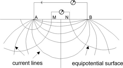
Figure 1.
Distribution of electric current in the half-space.
According to the Archie’s law, the apparent resistivity ρa (Ω m) of the ground, is determined (Eq. (1)):
where ΔV is the difference potential (V), I is the injected current (A), and K is a geometric factor depending on the electrodes arrangement.
The measured value ρa is an “apparent” resistivity because it refers to the resistivity of a homogeneous ground measured from a specific electrode arrangement. Apparent electrical resistivity is not a physical measurement, and the complex relationship with the “true” resistivity is obtained by solving the “inversion” problem.
Several electrical resistivity techniques are currently used with the quadrupole array. Here we focused on two different techniques: electrical resistivity tomography (ERT) and mise-a-la-masse (MALM).
2.1.1 Electrical resistivity tomography (ERT)
Electrical Resistivity Tomography (ERT) is the most widely used electrical technique for the subsurface imaging. More details about ERT technique are described in [72].
This technique combines a high sequence of quadrupole measurements in order to obtain a dense grid of apparent resistivity data according to a tomographic scheme (Figure 2). The observed data provide a qualitative representation of the subsurface electrical properties by contouring the apparent resistivity data. The “real” resistivity is achieved from inversion, that is a numerical technique that tries to determine a subsurface resistivity model by minimizing a generalized objective function, i.e., the misfit between the calculated (theoretical value) and observed (experimental value) data at the nodes of a mesh into which the subsurface is divided.
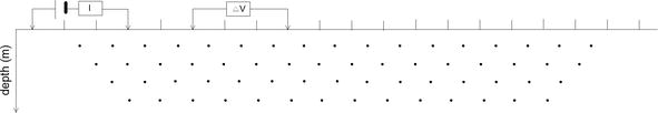
Figure 2.
Distribution of apparent electrical resistivity collected by a quadrupole array.
The resolution, i.e., the minimum distance at which a target can be detected, depends mainly on the inter-electrode spacing used for data collection, while the depth of investigation is influenced by the length of the ERT profile, the distance between current and potential dipoles, as well as the electrical properties of the investigated medium.
Depending on the data collection mode, along transects or in an area, the inverted model provides 2D or 3D resistivity model of the ground, which take into account lateral and vertical changes in the subsurface layers. Collecting resistivity data in time-lapse mode, i.e., repeating resistivity measurements over time along profiles or in an area, allows for monitoring spatiotemporal variations associated with dynamical processes.
2.1.2 Mise-a-la-masse (MALM)
Mise-a-la-masse is one of the oldest electrical resistivity techniques originally used to identify and map boundaries and orientation of electrically conductive ore bodies [73, 74, 75, 76].
In MALM technique, the four-electrode array is set up as follows: two electric currents are placed (A) inside the conductive target and (B) ideally at infinity, other two potential electrodes are placed (N) outside at infinity opposite of B and (M) is used to detect the edges of the underground target (Figure 3).
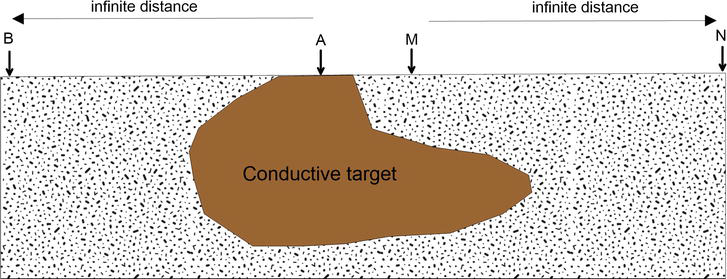
Figure 3.
Basics of MALM technique.
The electric current flows from inside to outside the target, and a potential map is recorded with reference to the electrode M.
When used for detecting the integrity of the HDPE liner laid down on the bottom of the landfill, no current pathways are recorded between the inner and outer parts of the landfill and, consequently, a zero potential gradient is measured if the liner has no ruptures. In case of lack, the electrical current moves toward the infinity electrode (B) across the rupture of the liner and a voltage map indicate the presence of current pathways between the inner and outer parts of the landfill.
2.2 Electromagnetic induction (EMI)
The EMI technique is based on the electromagnetic induction principle. An alternating current circulates in a transmitter loop coil T, generating a time-varying magnetic field, defined as the primary magnetic field (HP). This field induces eddy currents in a conductive body placed into the ground, which in turn generate a secondary magnetic field (HS), having an amplitude much smaller than that of the primary field. A receiver coil (R) measures the total complex electromagnetic response, i.e., the sum of both primary and secondary magnetic fields (Figure 4).
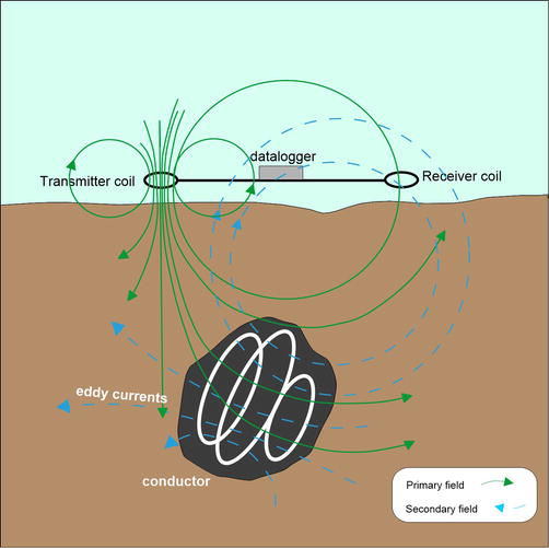
Figure 4.
Basics of EMI technique.
The real part, which has the same phase as the primary magnetic field, is called In-phase (P) component while the imaginary part, called Quadrature (Q) component, is 90° out-of-phase with the primary. The response parameter, called also “induction number,” indicated with β, depends on electrical resistivity, the magnetic permeability, the geometry of the buried body, and ω, the operating angular frequency of the current in the transmitter coil (Eq. (2)):
When β < <1, usually defined as “low induction number” (LIN) condition [77], the complex electromagnetic response can be simplified so that Q is linearly proportional to the electrical conductivity of the half-space
The response parameter is a function of the penetration depth of the signal, defined as the skin depth δ, that is the depth at which an electromagnetic signal attenuates by a value equal to 37% with respect to the initial value. It depends not only by the electromagnetic properties of the investigated medium but also on the coils distance. At the same time the depth of investigation is also a function of the coils orientation. When they are oriented perpendicular to the ground, the horizontal magnetic dipoles are in vertical coplanar configuration (VMD), which allows the investigation of the superficial layers. By rotating both coils by 90°, the vertical magnetic dipoles turn into horizontal coplanar position (HMD), which increases the investigation depth. As for raw ERT measurements, the data measured is an “apparent” electrical conductivity (ECa), i.e., it is the equivalent electrical conductivity of a homogeneous half-space that produces the same measured response to the instrument in a single configuration (coil distance, coil orientation, frequency). In addition, the high electrical conductivity of the waste deposits, combined with the high inter-coil distance necessary for increasing the depth of investigation, makes it impossible that the LIN condition is met, causing a nonlinear EM response of the half-space and leading to a data inversion procedure for modeling the landfill body.
3. Case studies
3.1 Corigliano d’Otranto landfill
The first case study concerns a dismissed quarry, located in Southern Italy, near the municipality of Corigliano d’Otranto (4451117 N–265375.00 E WGS UTM84), used as MSW landfill since late 1980s. During the excavation of a new landfill, bordering the old one, leachate came out at the base of the scarp, which separates the two landfills (Figure 5), clear evidence of the leaching out of the old landfill. Few direct information was available in the original landfill design: the waste thickness was no greater than 20 m from ground surface, and the existence of a barrier on the landfill bottom, proved by the presence of the impermeable HDPE liner, clearly visible along the South-West border of the landfill. These uncertainties requested the planning of a detailed geophysical investigation in order to evaluate the liner integrity at the landfill bottom and localize possible ruptures and spill points.
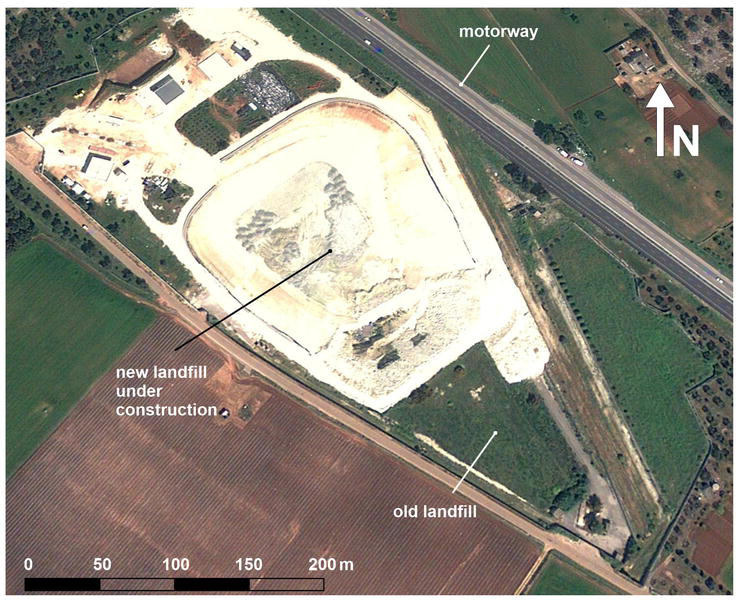
Figure 5.
The landfill area at Corigliano d’Otranto.
For this purpose, ERT and MALM survey were carried out (Figure 6). In particular, two ERT profiles, named Line 1 and Line 2, were carried out inside the landfill in order to identify the approximate thickness of the waste in the old quarry. Line 1 runs along the dirt road separating the old and new landfills, Line 2, almost perpendicular to Line 1, crosses both the old and the new landfills along the scarp between the two landfills. In addition, another ERT profile, Line 3, was carried out outside the landfill as a reference section for defining the resistivity distribution of the rocky subsurface not interested in waste deposits. ERT data were collected using an IRIS Syscal Pro 48 (Iris Instruments) resistivity meter, by planting 48 stainless steel electrodes into the ground with 5 m spacing and 235 m long array. A Wenner–Schlumberger configuration was used because it offers a reasonable compromise between resolution and investigation depth, about 40 m from the ground surface. Overall, more than 2000 resistance quadrupoles were collected for each profile, including direct acquisition and reciprocal data, i.e., by swapping current with potential dipoles, in order to provide a correct data error estimation [78]. In the preprocessing stage, data filtering has consisted in removing measurements that exceeded 10% of reciprocal error. Inversion of ERT data was run using the code ProfileR (A. Binley—Lancaster University), an inverse solution for a 2-D resistivity distribution based on computation of 3-D current flow using a quadrilateral finite element mesh. In addition, seven MALM profiles were performed inside the old landfill, with 2 m inter-electrode spacing in order to ensure a good spatial coverage of the whole area. Electric current was injected between electrodes A and B, and voltage was measured with reference to electrode P. Potential data were mapped using Surfer (Golden Software, LLC) code.
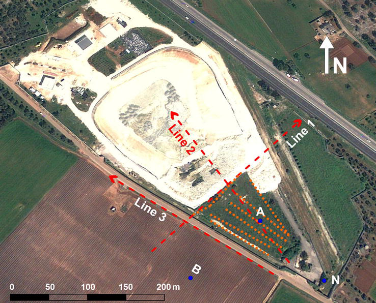
Figure 6.
Location of the ERT and MALM measurements carried out at the Corigliano site. The red dashed lines represent the 2D ERT profiles, while the orange dots indicate the location of the potential electrodes used for the MALM survey.
3.2 Ugento landfill
The second case study refers the geophysical investigation performed in the MSW landfill located in Ugento (4420400 N–2795270 E WGS UTM84). The landfill was built in the 1990s in an abandoned quarry of calcarenite, a sedimentary porous rock widespread in the Apulia Region. It is divided into three plots and covers a total area of about 9 hectares (Figure 7).
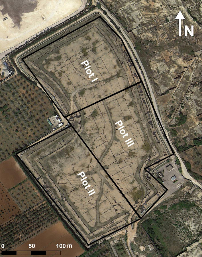
Figure 7.
The landfill area at Ugento site (image source: Google Earth).
The thickness of the waste body ranges from 15 m (plot I) to 19 m (plots II and III). An impermeable HDPE liner is laid down at the bottom and along the lateral boundary of each plot, as clearly visualized in the time-lapse historical Google Earth pictures of the landfill area. At the end of the operational stage, the Ugento landfill has been capped in order to prevent infiltration of rainwater into the waste that would increase the leachate production and gas dispersion in the air. The presence of the impermeable HDPE liner on the top surface inhibits any direct investigation and strongly limits the use of other indirect surveys. Being based on the electromagnetic induction principle, the EMI technique overcomes such strong limitations because it does not require any galvanic contact between probes and the ground. For this purpose, an EMI survey was planned using a CMD DUO device (GF Instruments), which consists of two independent coils, a transmitter, and a receiver, connected to each other by a flexible cable of different length, 10 m, 20 m, and 40 m, respectively, to deepen the electromagnetic signal into the waste deposits and the underlying vadose zone. Twenty-one EMI transects were collected either in a VMD or HMD configuration coil on the top of the landfill along parallel profiles in two orthogonal directions: 12 profiles in NW-SE direction, approximately 20 m apart, and 9 profiles in NE-SW direction, approximately 40 m apart (Figure 8). Continuous measurements mode, i.e. the data are collected while the instrument moves in the field, has been chosen by setting a time step equal to 2 s in order to obtain stable hence accurate measurements.
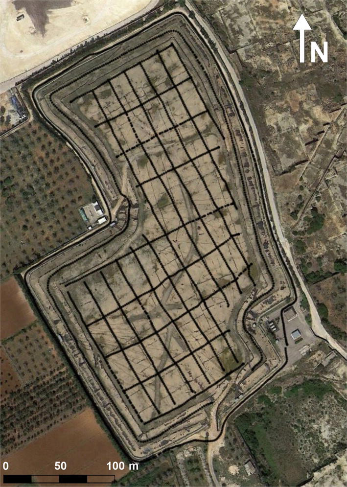
Figure 8.
Location of the EMI measurements carried out at the Ugento site. The black lines represent the 2D EMI transects (image source: Google Earth).
Overall, more than 11,000 measurements have been collected combining six different configurations, resulting in using three inter-coil spacings for each of the two coil configurations. Such data have been merged in order to obtain 1540 geometric depth soundings with six complex responses each, which, in turn, have been used for inversion. A free MATLAB software package, FDEMTool code [78], was used for inverting the electromagnetic data, and the resulting model was visualized with Voxler (Golden Software, LLC) code.
3.3 Asiago landfill
The MSW Asiago landfill (700550 N–5081863 E WGS UTM84) was developed since 2001 in a closed limestone quarry. The landfill has an area of about 1.5 hectares with a perimeter of about 500 m, and a maximum thickness of the waste deposits of about 40 m. The landfill was closed in mid-2018, and ever since it is a totally closed system due to the presence of HDPE liners at its bottom and at its top surface (Figure 9).
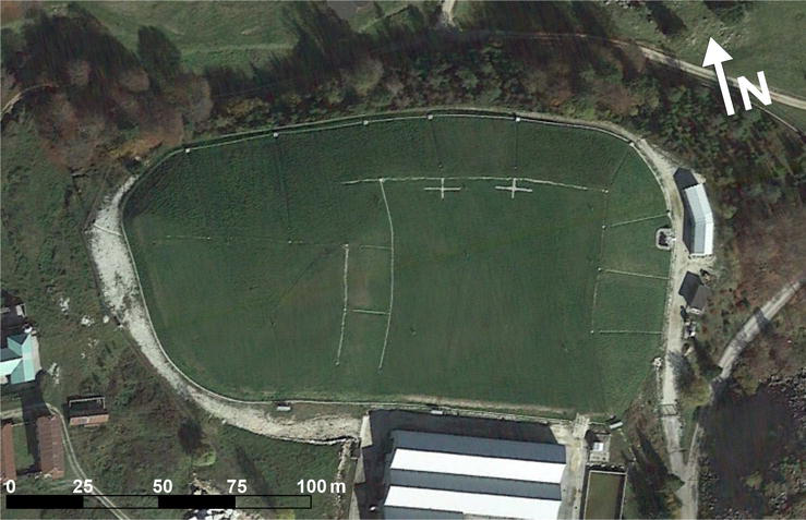
Figure 9.
The landfill area at Asiago site (image source: Google earth).
Clear evidence of karstic phenomena reported in the area of the landfill site raised concern for the possible presence of large karstic cavities below the landfill and, secondarily, possible pathways for leachate contamination through the limestone fractured system. In search of possible large karstic cavities and possible leachate leaks, an ERT survey was proposed and implemented. As data collection from the top surface of the landfill body was made impossible by the presence of the impermeable (and electrically insulating) HDPE liner, an unconventional electrode configuration has been chosen by placing 101 electrodes all around the perimeter of the landfill body (Figure 10).
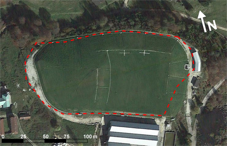
Figure 10.
Location of 101 electrodes placed around the perimeter of the landfill body (dashed red line) at the Asiago landfill site (image source: Google Earth).
A Syscal Pro (Iris Instruments) resistivimeter was used for the data collection. Overall, more than 12,000 resistivity measurements were collected, including reciprocals, to evaluate data quality. Data filtering rejected bad data points that overcome threshold values equal to 10% of reciprocal error and measured voltages less than 10−6 V. The survey geometry was designed on the basis of preliminary synthetic modeling based on a 3D model of electrical current diffusion in a heterogeneous medium. The purpose was to verify whether the proposed approach was capable of imaging large karstic cavities (of a diameter around 20 m) and thus identify a viable acquisition and inversion strategy. Three scenarios, based on the presence of a cavity below the bottom of the landfill at different locations, were simulated. This posed the basis for a comparison with the results from real observed data.
4. Results
4.1 Corigliano d’Otranto landfill
The inverted ERT cross-sections clearly show the electrical behavior of the waste deposits and the rocky subsurface. Line 3, located outside the landfill and hence not involved in waste deposits, highlights a homogeneous distribution of the electrical resistivity, with a narrow range, expressed in logarithmic scale, varying from 2.6 and 3 Ω m, typically associated with the porous rock that constitutes the vadose subsurface (Figure 11a). On the contrary, Lines 2 and 1 (Figure 11b and c, respectively) put in evidence a very high conductive structure, with log10 resistivity approximately below 1.6 Ω m, clearly associated with the waste deposits located in the old landfill. Differences between the two ERT cross-sections are observed. In particular, while in Line 2, the conductive body is confined within the 20 m from top surface, Line 1, which cuts the scarp along its maximum slope, shows a conductive body deepening much more than the expected depth of the HDPE liner (dashed black line), about 20 m from the top surface. This difference can be explained by the fact that Line 1 violates the assumption, always made in 2D ERT, that the ground perpendicular to the survey line is homogeneous. In fact, the presence of waste deposits located in the old landfill on one side of the profile and the free space (air) on the other side of Line 1 masks the true thickness of the waste deposits.
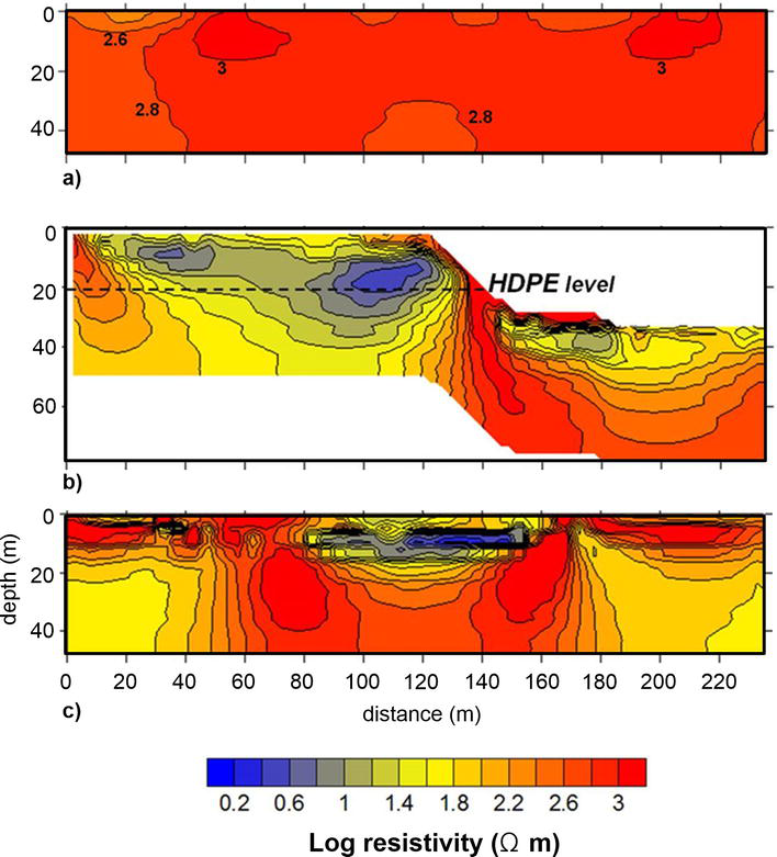
Figure 11.
2D ERT cross-section from: (a) Line 3; (b) Line 2; (c) Line 1.
On the other hand, this assumption is verified in Line 2, and the corresponding ERT cross-section provides a correct quantitative interpretation of the thickness of the waste deposits. The scenario derived from Line 2 indicates a vertical migration of conductive leachate which penetrates the supposed impermeable landfill bottom. The MALM provides further information about the structure of the landfill body. The potential map shows a sharp voltage jump in correspondence with the limits of the old landfill, in particular across the visible emergence of the HDPE liner along the South–West boundary (Figure 12).
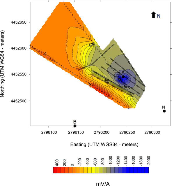
Figure 12.
Potential map obtained from MALM survey.
This evidence could be due to the poor confinement close to ground surface, considered that no other evidence of the liner is present on the ground surface. As the MALM results do not clearly support the ERT findings, in order to corroborate the hypothesis of the rupture of the impermeable HDPE liner, different alternative interpretation scenarios have been compared with numerical modeling. Figure 13 shows the simulations of the geophysical modeling (ERT—Line 2 and MALM) in case of undamaged and damaged HDPE liner scenario, respectively. The simulated MALM maps do not show significant differences with the observed maps in both predicted scenarios (Figure 13c and d compared with Figure 12), probably due to the poor lateral confinement previously mentioned. On the other hand, the simulation of the ERT—Line 2 cross clearly highlights a good agreement in case of damaged HDPE liner scenario (Figures 11b and 13b), thus leading to reasonably assume the hypothesis of a rupture of the HDPE liner through which the current flows.
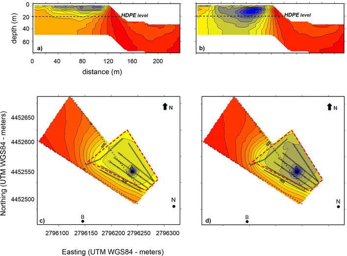
Figure 13.
Simulated ERT—Line 2 cross-section and MALM potential map in case of undamaged HDPE liner scenario (
4.2 Ugento landfill
The distribution of the electrical conductivity in the landfill body is visualized by a 3D image (Figure 14). It can be schematized into a three-layers model: (a) upper highly conductive; (b) weakly conductive intermediate; (c) resistive lower layer.
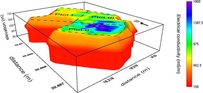
Figure 14.
3D electrical conductivity model of Ugento landfill.
The visualization of the findings through 2D vertical cross sections (Figure 15) better highlights the upper conductive layer, with values from 1000 mS/m to 1800 mS/m, and the lower resistive layer, having lower values to about 150 mS/m.
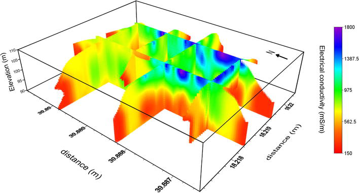
Figure 15.
3D visualization of the electrical conductivity model through 2d vertical cross sections.
Depth slices at different depths put in evidence details of the electrical conductivity inside the landfill (Figure 16).
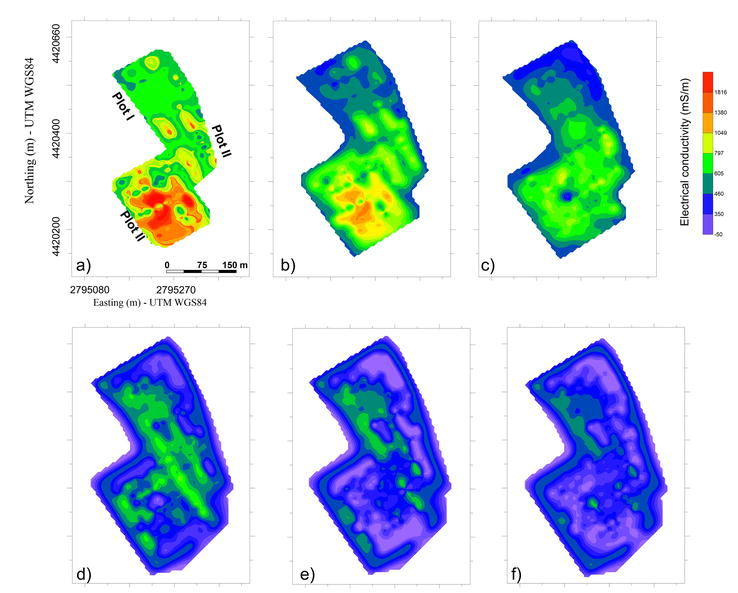
Figure 16.
2D depth slices extracted from the 3D EC model: (a) z = 1 m from ground surface; (b) z = 2 m from ground surface; (c) z = 5 m; (d) z = 10 m; (e) z = 15 m; and (f) z = 20 m.
The highly conductive upper layer has a maximum thickness of 5 m and an average EC ≈ 1200 mS/m (Figure 16a and b). The observed heterogeneity is probably associated with different waste composition, probably due to organic waste, a higher moisture content or a different compaction of the waste body by means of compacting trucks. The weakly conductive intermediate layer ranges from 5 m to 10 m from ground surface with an average value of EC ≈ 500 mS/m (Figure 16c and d). The waste deposits highlight a gradual decreasing in conductivity, explained by the loss of water in the waste body due to the weight of the overburden mass and then collected by the pipelines at the bottom of the landfill, and/or with the limited content of materials with high surface conductivity. Finally, the resistive lower layer (bedrock) deepens up to the maximum investigation depth with minimum EC ≈ 150 mS/m. In particular, no significant variations in the inverted electromagnetic signal were recorded in this portion of the subsurface (Figure 16e and f). Any expected high conductivity signal, linked to accumulation of leachate, is detected at depth, thus ensuring their absence.
4.3 Asiago landfill
The field acquisition at the Asiago landfill was conducted in one day (June 1, 2019) following the same configuration that proved most effective in the synthetic exercise, i.e., a total of 101 electrodes with a full dipole-dipole skip-12 configuration, that corresponds to a dipole length of 13 × 5 m = 65 m. Figure 17 shows the results of the inversion of real field data. No significant high resistivity anomalies, associated with potential karstic cavities, have been detected, leading to exclude their presence. However, as a side result, the ERT survey showed the presence of a low-resistivity zone in the downhill portion of the landfill, as highlighted in the red circle: note that in this region, very close to the electrodes themselves, the sensitivity is particularly high. This area also corresponds to a low in the topography of the quarry where the landfill was developed. Since this high conductivity anomaly could be linked to the presence of leachate, a direct investigation was planned and performed in July 2021: the drilled core showed the presence of fine sediments (silt and clay) accumulated in this area of valley bottom, and the presence of freshwater probably coming from uphill in the valley, with no relationship with the landfill itself.
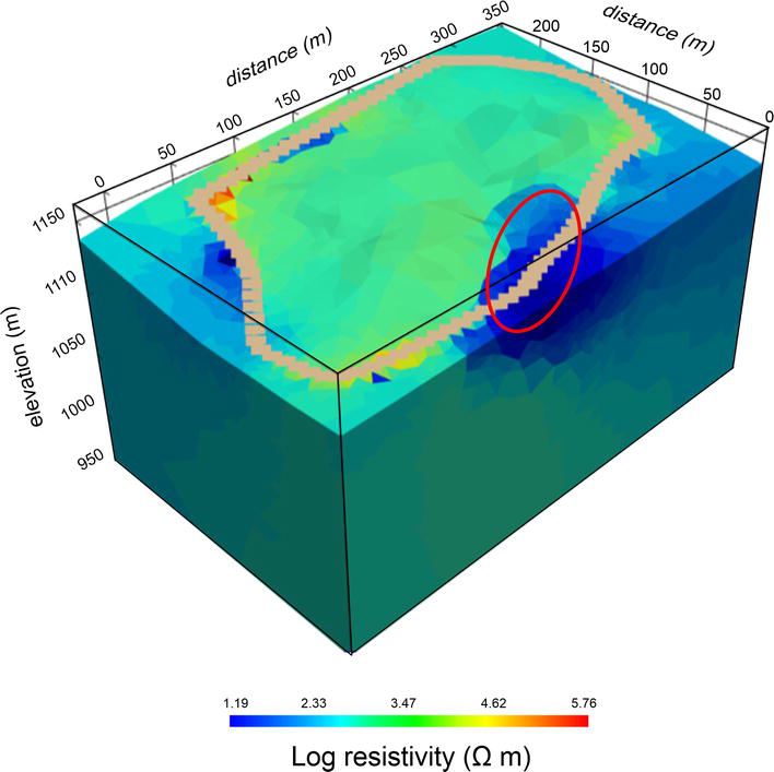
Figure 17.
Inverted resistivity model, expressed in log scale.
The real 3D resistivity image, compared against the expected image (Figure 18) in the presence of a 20 m diameter cavity, confirms that no such cavity exists below the landfill. Smaller cavities, if present, would have no substantial impact on the mechanical stability of the system. As the presence of karstic cavities was the main goal of the investigation, one could conclude that the survey confirmed that no such feature is present at the site.
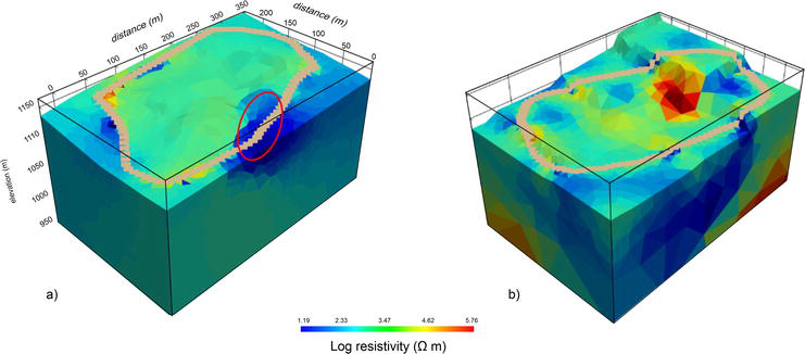
Figure 18.
Comparison between inverted (a) and simulated (b) ERT model.
5. Conclusion
In the context of the study of abandoned or dismissed landfill, the lack of crucial information concerning landfill design and waste body characterization makes difficult the development of an accurate site conceptual model. Clear evidence about the presence of the HDPE impermeable liner on the bottom of the landfill and its possible integrity, as well as uncertainty on information regarding the structure of the waste deposits, are often missing. Noninvasive geophysical techniques have proved to be an effective tool to “see” inside the waste deposits in order to provide useful information about their physical properties with an accuracy degree unattainable with other technique. A huge amount of data can be collected over large areas in a short time in order to image the thickness of the covering layer, the geometry of the waste deposits, type of waste, and potential accumulation zones. In addition, data collected in time-lapse mode allows for monitoring hydrodynamic processes taking place inside landfill body. In this chapter, three case studies showing different site conditions have been described in order to highlight the potentialities and the versatility of the geophysical techniques in the study of landfills. In the Corigliano d’Otranto landfill, ERT and MALM measurements have been collected inside and outside the landfill to estimate the thickness of the waste deposits, verify the confinement of the waste deposits above the impermeable HDPE liner and, in case of rupture, image the leachate infiltration in the underlying vadose zone. The ERT outcomes highlight a very low-resistivity structure (less than 10 Ω m), associated to the waste deposits, one order of magnitude lower than the rocky subsurface. The thickness of this conductive structure is about 40 m, much more than the expected 20 m, leading to hypothesize a rupture of the impermeable HDPE liner and a vertical migration of landfill leachate through the landfill bottom. On the other hand, the potential map obtained from MALM measurements cannot clearly confirm such hypothesis, due to the lack of insulation in the shallow layer covering the waste mass which causes a current flow from inside to outside of the landfill. In such cases, when logistical limitations strongly affect the geophysical data acquisition and interpretation, forward numerical modeling provides added value to the geophysical data, by simulating different alternative interpretation scenarios. The good agreement between simulated and observed data in case of damaged HDPE liner leads to reasonably assume the hypothesis of a rupture of the bottom liner through which the current flows. In the capped Ugento landfill, the presence of the HDPE impermeable liner on the top surface strongly limits any direct investigation. The EMI measurements allowed to gain information about the waste composition, the thickness of the waste deposits and integrity of the HDPE liner. The electromagnetic model pointed out heterogeneities in the waste deposits located on the top layers, where highly conductive signal is associated with different waste composition, organic waste, or a higher moisture content. The electrical conductivity decreases with depth, probably due to the loss of water caused by compaction induced by the weight of the overburden mass. No significant conductivity anomalies have been observed in the expected transition depth between the upper waste deposits and the lower bedrock. This evidence leads to exclude ruptures of the HDPE liner placed at the bottom of the landfill because a leachate migration below the landfill bottom would cause large electrical conductivity anomalies in the bedrock. The Asiago landfill case shows how a careful planning of geophysical measurements is essential in order to produce the best strategy for achieving the set goal in such complex sites, and in particular in order to confirm/dismiss an hypothesis concerning the landfill and its subsurface, in this case the presence of a large karstic cavity. In addition, the survey showed also some unexpected results, i.e., the presence of a low-resistivity anomaly that, in the context of landfills, is a general warning sign, as leachate may produce low conductivity anomalies in the surrounding of a landfill, in presence of a leakage. In this case, this anomaly seen by geophysics has driven a direct investigation that ensured that the anomaly itself has no relationship with the landfill. Overall this is an example of a virtuous circle between noninvasive and invasive investigations, as it should be. The results encourage the use of geophysical data, both for static characterization and dynamic monitoring as good practices for checking the health condition of a landfill facility in order to minimize public health risks, ensure environmental protection and avoid expensive reclamation activities.
Integrating the geophysical information with routine environmental matrices monitoring as defined by the community regulations can represent an optimal strategy for the development of a site conceptual model essential in the management of waste landfill both in operational and postoperational stages.
Acknowledgments
The authors wish to thank the managers of the three landfill sites (Monteco srl, manager of the Ugento landfill, Progetto Ambiente Bacino Lecce DUE s.r.l, manager of the Corigliano d’Otranto landfill, and the Alto Vicentino Ambiente manager of the Asiago landfill) for making the facility available to carry out the geophysical measurements. Moreover, all authors wish to thank the Apulian Regional Agency for the Protection of the Environment (ARPA PUGLIA) for funding the research at the Ugento landfill, the Municipality of Asiago (VI) for funding the research at the Asiago landfill, for granting permission for the publication of the results and funding direct drilling investigation, the Progetto Ambiente Bacino Lecce DUE s.r.l for funding the research activities at the Corigliano d’Otranto landfill. In addition, the authors wish to thank Celeste Antonietta Turturro, Jacopo Boaga, and Benjamin Mary for supporting the field experimental activity.
References
- 1.
Soupios P, Papadopoulos I, Kouli M, Georgaki I, Vallianatos F, Kokkinou E. Investigation of waste disposal areas using electrical methods: A case study from Chania, Crete, Greece. Environmental Geology. 2007; 51 :1249-1261. DOI: 10.1007/s00254-006-0418-7 - 2.
Chambers JE, Kuras O, Meldrum PI, Ogilvy RD, Hollands J. Electrical resistivity tomography applied to geologic, hydrogeologic, and engineering investigations at a former waste-disposal site. Geophysics. 2006; 71 :B231-B239. DOI: 10.1190/1.2360184 - 3.
Gazoty A, Fiandaca G, Pedersen J, Auken E, Christiansen AV. Mapping of landfills using time-domain spectral induced polarization data: The Eskelund case study. Near Surface Geophysics. 2012; 10 :575-586. DOI: 10.3997/1873-0604.2012046 - 4.
Meju MA. Geoelectrical investigation of old/abandoned, covered landfill sites in urban areas: Model development with a genetic diagnosis approach. Journal of Applied Geophysics. 2000; 44 :115-150. DOI: 10.1016/S0926-9851(00)00011-2 - 5.
Frid V, Doudkinski D, Liskevich G, Shafran E, Averbakh A, Korostishevsky N, et al. Geophysical–geochemical investigation of fire-prone landfills. Environmental Earth Sciences. 2010; 60 :787-798. DOI: 10.1007/s12665-009-0216-0 - 6.
Frid V, Liskevich G, Doudkinski D, Korostishevsky N. Evaluation of landfill disposal boundary by means of electrical resistivity imaging. Environmental Geology. 2008; 53 :1503-1508. DOI: 10.1007/s00254-007-0761-3 - 7.
Casado I, Mahjoub H, Lovera R, Fernandez J, Casas A. Use of electrical tomography methods to determinate the extension and main migration routes of uncontrolled landfill leachates in fractured areas. Science of the Total Environment. 2015; 506 :546-553. DOI: 10.1016/j. scitotenv.2014.11.068 - 8.
Deidda GP, Himi M, Barone I, Cassiani G, Casas PA. Frequency-domain electromagnetic mapping of an abandoned waste disposal site: A case in Sardinia (Italy). Remote Sensing. 2022; 14 :878. DOI: 10.3390/rs14040878 - 9.
De Iaco R, Green AG, Maurer HR, Horstmeyer H. A combined seismic reflection and refraction study of a landfill and its host sediments. Journal of Applied Geophysics. 2003; 52 :139-156. DOI: 10.1016/S0926-9851(02)00255-0 - 10.
Lanz E, Maurer H, Green A.G. Refraction tomography over a buried waste disposal site. Geophysics 1998:63:1414–1433. DOI: 10.1190/1.1444443 - 11.
Abreu AES, Gandolfo OCB, Vilar OM. Characterizing a Brazilian sanitary landfill using geophysical seismic techniques. Waste Management. 2016; 53 :116-127. DOI: 10.1016/j.wasman.2016.03.048 - 12.
Di Maio R, Fais S, Ligas P, Piegari E, Raga R, Cossu R. 3D geophysical imaging for site-specific characterization plan of an old landfill. Waste Management. 2018; 76 :629-642. DOI: 10.1016/j.wasman.2018.03.004 - 13.
Cardarelli E, Bernabini M. Two case studies of the determination of parameters of urban waste dumps. Journal of Applied Geophysics. 1997; 36 :167-174. DOI: 10.1016/S0926-9851(96)00056-0 - 14.
Dumont G, Robert T, Marck N, Nguyen F. Assessment of multiple geophysical techniques for the characterization of municipal waste deposit sites. Journal of Applied Geophysics. 2017; 145 :74-83. DOI: 10.1016/j.jappgeo.2017.07.013 - 15.
Kondracka M, Stan-Kłeczek I, Sitek S, Ignatiuk D. Evaluation of geophysical methods for characterizing industrial and municipal waste dumps. Waste Management. 2021; 125 :27-39. DOI: 10.1016/j.wasman.2021.02.015 - 16.
Leroux V, Dahlin T, Svensson M. Dense resistivity and induced polarization profiling for a landfill restoration project at Harlov, Southern Sweden. Waste Management and Research. 2007; 25 :49-60. DOI: 10.1177/0734242X07073668 - 17.
Carpenter PJ, Calkin SF, Kaufmann RS. Assessing a fractured landfill cover using electrical resistivity and seismic refraction techniques. Geophysics. 1991; 56 :1896-1904. DOI: 10.1190/1.1443001 - 18.
White CC, Barker RD. Electrical leak detection system for landfill liners: A case history. Ground Water Monitoring and Remediation. 1997; 17 :153-159. DOI: 10.1111/j.1745-6592.1997.tb00590.x - 19.
Binley A, Daily W, Ramirez A. Detecting leaks from waste storage ponds using electrical tomographic methods. In: Proceedings of the 1st World Congress on Industrial Process Tomography; 14–17 April 1999. Greater Manchester: Buxton; 1999, 1999. pp. 6-13 - 20.
Binley A, Daily W, Ramirez A. Detecting leaks from environmental barriers using electrical current imaging. Journal of Environmental and Engineering Geophysics. 1997; 2 :11-19. DOI: 10.4133/JEEG2.1.11 - 21.
Colucci P, Darilek GT, Laine DL, Binley A. Locating landfill leaks covered with waste. In: Proceedings of the Sardinia 99, Seventh International Waste Management and Landfill Symposium; 4–8 October 1999. Cagliari, Italy: CISA, Environmental Sanitary Engineering Centre; 1999. pp. 137-140 - 22.
Frangos W. Electrical detection of leaks in lined waste disposal ponds. Geophysics. 1997; 62 :1737-1744. DOI: 10.1190/1.1444274 - 23.
Laine DL, Binley AM, Darilek GT. How to Locate Liner Leaks Under Waste, Geotechnical Fabrics Report, 1997. Available from: https://trid.trb.org/view/576599 [Accessed: February 10, 2023] - 24.
Laine DL, Darilek GT, Binley AM. Locating Geomembrane liner leaks under waste in a landfill. In: Proceedings of the International Geosynthetics ‘97 Conference; 11–13 March 1997. Long Beach, USA; 1997. pp. p407-p411 - 25.
Parra JO. Electrical response of a leak in a geomembrane liner. Geophysics. 1988; 53 :1445-1452. DOI: 10.1190/1.1442424 - 26.
Binley A, Daily W. The performance of electrical methods for assessing the integrity of geomembrane liners in landfill caps and waste storage ponds. Journal of Environmental and Engineering Geophysics. 2003; 8 :227. DOI: 10.4133/JEEG8.4.227 - 27.
De Carlo L, Perri MT, Caputo MC, Deiana R, Vurro M, Cassiani G. Characterization of a dismissed landfill via electrical resistivity tomography and mise-à-la-masse method. Journal of Applied Geophysics. 2013; 98 :1-10. DOI: 10.1016/j.jappgeo.2013.07.010 - 28.
Cassiani G, Fusi N, Susanni D, Deiana R. Vertical radar profiles for the assessment of landfill capping effectiveness. Near Surface Geophysics. 2008; 6 :133-142. DOI: 10.3997/1873-0604.2008010 - 29.
Deidda GP, De Carlo L, Caputo MC, Cassiani G. Frequency domain electromagnetic induction imaging: An effective method to see inside a capped landfill. Waste Management. 2022; 144 :29-40. DOI: 10.1016/j.wasman.2022.03.007 - 30.
Zume JT, Tarhule A, Christenson S. Subsurface imaging of an abandoned solidwaste landfill site in Norman, Oklahoma. Ground Water Monitoring and Remediation. 2006; 26 :62-69. DOI: 10.1111/j.1745-6592.2006.00066.x - 31.
Radulescu M, Valerian C, Yang J. Time-lapse electrical resistivity anomalies due to contaminant transport around landfills. Annals of Geophysics. 2007; 50 :453-468. DOI: 10.4401/ag-3075 - 32.
Ogilvy R, Meldrum P, Chambers J, Williams G. The use of 3D electrical resistivity tomography to characterise waste and leachate distributions within a closed landfill Thriplow, UK. Journal of Environmental and Engineering Geophysics. 2002; 7 :11-18. DOI: 10.4133/JEEG7.1.11 - 33.
Lopes DD, Silva SMCP, Fernandes F, Teixeira RS, Celligoi A, Dall’Antônia LH. Geophysical technique and groundwater monitoring to detect leachate contamination in the surrounding area of a landfill—Londrina (PR—Brazil). Journal of Environmental Management. 2012; 113 :481-487. DOI: 10.1016/j.jenvman.2012.05.028 - 34.
Nobes DC, Armstrong MJ, Close ME. Delineation of a landfill leachate plume and flow channels in coastal sands near Christchurch, New Zealand, using a shallow electromagnetic survey method. Hydrogeology Journal. 2000; 8 :328-336. DOI: 10.1007/s100400050018 - 35.
Triantafilis J, Roe JAE, Monteiro Santos FA. Detecting a leachate plume in an Aeolian sand landscape using a DUALEM-421 induction probe to measure electrical conductivity followed by inversion modeling. Soil Use and Management. 2011; 27 :357-366. DOI: 10.1111/j.1475-2743.2011.00352.x - 36.
Bavusi M, Rizzo E, Lapenna V. Electromagnetic methods to characterize the Savoia di Lucania waste dump (southern Italy). Environmental Geology. 2006; 51 :301-308. DOI: 10.1007/s00254-006-0327-9 - 37.
Monteiro Santos FA, Mateus A, Figueiras J, Gonçalves MA. Mapping groundwater contamination around a landfill facility using the VLF-EM method — A case study. Journal of Applied Geophysics. 2006; 60 :115-125. DOI: 10.1016/j.jappgeo.2006.01.002 - 38.
Porsani JL, Filho WM, Elis VR, Shimeles F, Dourado JC, Moura HP. The use of GPR and VES in delineating a contamination plume in a landfill site: A case study in SE Brazil. Journal of Applied Geophysics. 2004; 55 :199-209. DOI: 10.1016/j.jappgeo.2003.11.001 - 39.
Faraco Gallas JD, Taioli F, Malagutti FW. Induced polarization, resistivity, and self-potential: A case history of contamination evaluation due to landfill leakage. Environmental Earth Sciences. 2011; 63 :251-261. DOI: 10.1007/s12665-010-0696-y - 40.
Soupios P, Papadopoulos N, Papadopoulos I, Kouli M, Vallianatos F, Sarris A, et al. Application of integrated methods in mapping waste disposal areas. Environmental Geology. 2007; 53 :661-675. DOI: 10.1007/s00254-007-0681-2 - 41.
Audebert M, Clément R, Moreau S, Duquennoi C, Loisel S, Touze-Foltz N. Understanding leachate flow in municipal solid waste landfills by combining time-lapse ERT and subsurface flow modelling—Part I: Analysis of infiltration shape on two different waste deposit cells. Waste Management. 2016; 55 :165-175. DOI: 10.1016/j.wasman.2016.04.006 - 42.
Audebert M, Oxarango L, Duquennoi C, Touze-Foltz N, Forquet N, Clément R. Understanding leachate flow in municipal solid waste landfills by combining time-lapse ERT and subsurface flow modelling—Part II: Constraint methodology of hydrodynamic models. Waste Management. 2016; 55 :176-190. DOI: 10.1016/j.wasman.2016.04.005 - 43.
Acworth RI, Jorstad LB. Integration of multi-channel piezometry and electrical tomography to better define chemical heterogeneity in a landfill leachate plume within a sand aquifer. Journal of Contaminant Hydrology. 2006; 83 :200-220. DOI: 10.1016/j.jconhyd.2005.11.007 - 44.
Aristodemou E, Thomas-Betts A. DC resistivity and induced polarisation investigations at a waste disposal site and its environments. Journal of Applied Geophysics. 2000; 44 :275-302. DOI: 10.1016/S0926-9851(99)00022-1 - 45.
Al-Tarazi E, Abu Rajab J, Al-Naqa A, El-Waheidi M. Detecting leachate plumes and groundwater pollution at Ruseifa municipal landfill utilizing VLF-EM method. Journal of Applied Geophysics. 2008; 65 :121-131. DOI: 10.1016/j.jappgeo.2008.06.005 - 46.
Hu X, Han Y, Wang Y, Zhang X, Du L. Experiment on monitoring leakage landfill leachate by parallel potentiometric monitoring method. Scientific Reports. 2022; 12 :20496. DOI: 10.1038/s41598-022-24352-w - 47.
Grellier S, Guérin R, Robain H, Bobachev A, Vermeersch F, Tabbagh A. Monitoring of leachate recirculation in a bioreactor landfill by 2-D electrical resistivity imaging. Journal of Environmental and Engineering Geophysics. 2008; 13 :351-359. DOI: 10.2113/JEEG13.4.351 - 48.
Konstantaki LA, Ghose R, Draganov D, Diaferia G, Heimovaara T. Characterization of a heterogeneous landfill using seismic and electrical resistivity data. Geophysics. 2015; 80 :EN13-EN25. DOI: 10.1190/GEO2014-0263.1 - 49.
Hermozilha H, Grangeia C, Matias MS. An integrated 3D constant offset GPR and resistivity survey on a sealed landfill — Ilhavo, NW Portugal. Journal of Applied Geophysics. 2010; 70 :58-71. DOI: 10.1016/j.jappgeo.2009.11.004 - 50.
Mota R, Monteiro Santos FA, Mateus A, Marques FO, Gonçalves MA, Figueiras J, et al. Granite fracturing and incipient pollution beneath a recent landfill facility as detected by geoelectrical surveys. Journal of Applied Geophysics. 2004; 57 :11-22. DOI: 10.1016/j.jappgeo.2004.08.007 - 51.
Olofsson B, Jernberg H, Rosenqvist A. Tracing leachates at waste sites using geophysical and geochemical modelling. Environmental Geology. 2006; 49 :720-732. DOI: 10.1007/s00254-005-0117-9 - 52.
Osiensky JL. Ground water modeling of mise-à-la-masse delineation of contaminated ground water plumes. Journal of Hydrology. 1997; 197 :146-165. DOI: 10.1016/S0022-1694(96)03279-9 - 53.
Manzur SR, Hossain MS, Kemler V, Khan MS. Monitoring extent of moisture variations due to leachate recirculation in an ELR/bioreactor landfill using resistivity imaging. Waste Management. 2016; 55 :38-48. DOI: 10.1016/j.wasman.2016.02.035 - 54.
Clément R, Descloitres M, Günther T, Oxarango L, Morra C, Laurent JP, et al. Improvement of electrical resistivity tomography for leachate injection monitoring. Waste Management. 2010; 30 :452-464. DOI: 10.1016/j.wasman.2009.10.002 - 55.
Clément R, Oxarango L, Descloitres M. Contribution of 3-D time-lapse ERT to the study of leachate recirculation in a landfill. Waste Management. 2011; 31 :457-467. DOI: 10.1016/j.wasman.2010.09.005 - 56.
Guérin R, Munoz ML, Aran C, Laperrelle C, Hidra M, Drouart E, et al. Leachate recirculation: Moisture content assessment by means of a geophysical technique. Waste Management. 2004; 24 :785-794. DOI: 10.1016/j.wasman.2004.03.010 - 57.
Audebert M, Clément R, Grossin-Debattista J, Günther T, Touze-Foltz N, Moreau S. Influence of the geomembrane on time-lapse ERT measurements for leachate injection monitoring. Waste Management. 2014; 34 :780-790. DOI: 10.1016/j.wasman.2014.01.011 - 58.
Degueurce A, Clément R, Moreau S, Peu P. On the value of electrical resistivity tomography for monitoring leachate injection in solid state anaerobic digestion plants at farm scale. Waste Management. 2016; 56 :125-136. DOI: 10.1016/j.wasman.2016.06.028 - 59.
Jansen J, Haddad B, Fassbender W, Jurcek P. Frequency domain electromagnetic induction sounding surveys for landfill site characterization studies. Groundwater Monitoring and Remediation. 1992; 12 :103-109. DOI: 10.1111/j.1745-6592.1992.tb00068.x - 60.
Yannah M, Martens K, Van Camp M, Walraevens K. Geophysical exploration of an old dumpsite in the perspective of enhanced landfill mining in Kermt area, Belgium. Bulletin of Engineering Geology and the Environment. 2019; 78 :55-67. DOI: 10.1007/s10064-017-1169-2 - 61.
Yochim A, Zytner RG, McBean EA, Endres AL. Estimating water content in an active landfill with the aid of GPR. Waste Management. 2013; 33 :2015-2028. DOI: 10.1016/j.wasman.2013.05.020 - 62.
Kibria G, Hossain MS. Investigation of degree of saturation in landfill liners using electrical resistivity imaging. Waste Management. 2015; 29 :197-204. DOI: 10.1016/j.wasman.2015.02.015 - 63.
Steiner M, Katona T, Fellner J, Flores OA. Quantitative water content estimation in landfills through joint inversion of seismic refraction and electrical resistivity data considering surface conduction. Waste Management. 2022; 149 :21-32. DOI: 10.1016/j.wasman.2022.05.020 - 64.
Dumont G, Pilawski T, Dzaomuho-Lenieregue P, Hiligsmann S, Delvigne F, Thonart P, et al. Gravimetric water distribution assessment from geoelectrical methods (ERT and EMI) in municipal solid waste landfill. Waste Management. 2016; 55 :129-140. DOI: 10.1016/j. wasman.2016.02.013 - 65.
Imhoff PT, Reinhart DR, Englund M, Guerin R, Gawande N, Han B, et al. Review of state of the art methods for measuring water in landfills. Waste Management. 2007; 27 :729-745. DOI: 10.1016/j.wasman.2006.03.024 - 66.
Flores-Orozco A, Gallistl J, Steiner M, Brandstätter C, Fellner J. Mapping biogeochemically active zones in landfills with induced polarization imaging: The Heferlbach landfill. Waste Management. 2020; 107 :121-132. DOI: 10.1016/j.wasman.2020.04.001 - 67.
Georgaki I, Soupios P, Sakkas N, Ververidis F, Trantas E, Vallianatos F, et al. Evaluating the use of electrical resistivity imaging technique for improving CH 4 and CO 2 emission rate estimations in landfills. Science of the Total Environment. 2008; 389 :522-531. DOI: 10.1016/j.scitotenv.2007.08.033 - 68.
Johansson S, Rosqvist H, Svensson M, Dahlin T, Leroux V. An alternative methodology for the analysis of electrical resistivity data from a soil gas study. Geophysical Journal International. 2011; 186 :632-640. DOI: 10.1111/j.1365-246X.2011.05080 - 69.
Noguera JF, Rivero L, Font X, Navarro A, Martínez F. Simultaneous use of geochemical and geophysical methods to characterise abandoned landfills. Environmental Geology. 2002; 41 :898-905. DOI: 10.1007/s00254-001-0467-x - 70.
Senos Matias M, Marques da Silva M, Ferreira P, Ramalho E. A geophysical and hydrogeological study of aquifers contamination by a landfill. Journal of Applied Geophysics. 1994; 32 :155-162. DOI: 10.1016/0926-9851(94)90017-5 - 71.
Binley A, Kemna A. DC resistivity and induced polarization methods. In: Rubin Y, Hubbard SS, editors. Hydrogeophysics. 1st ed. Dordrecht: Springer; 2005. pp. 129-156 - 72.
Schlumberger C. Ètude sur la prospection electrique du sous-sol. 1st ed. Paris: Gauthier-Villars; 1920. pp. 1-94 - 73.
Parasnis DS. Three-dimensional electric mise-a-la-masse survey of an irregular lead–zinc–copper deposit in Central Sweden. Geophysical Prospecting. 1967; 15 :407-437. DOI: 10.1111/j.1365-2478.1967.tb01796.x - 74.
Ketola M. Some points of view concerning mise-a-la-masse measurements. Geoexploration. 1972; 10 :1-21. DOI: 10.1016/0016-7142(72)90010-5 - 75.
Bowker A. Size determination of slab-like ore bodies an interpretation scheme for single hole mise-a-la-masse anomalies. Geoexploration. 1987; 24 :207-218. DOI: 10.1016/0016-7142(87)90028-7 - 76.
McNeill JD. Electromagnetic terrain conductivity measurements at low induction numbers. Technical Note TN-6. 1980. Available from: http://www.geonics.com/pdfs/technicalnotes/tn6.pdf [Accessed: 10 January 2020] - 77.
Binley A, Ramirez A, Daily W. Regularised image reconstruction of noisy electrical resistance tomography data. In: Proceedings of the 4th Workshop of the European Concerted Action on Process Tomography. Bergen: UMIST, University of Manchester Institute of Science and Technology; 1995. pp. 401-410 - 78.
Deidda GP, Díaz de Alba P, Fenu C, Lovicu G, Rodriguez G. FDEMtools: A MATLAB package for FDEM data inversion. Numerical Algorithms. 2020; 84 :1313-1327. DOI: 10.1007/s11075-019-00843-2