Application of Optimal Solutions in Field-Oriented Control of Induction Motor

Abstract

This chapter presents the optimal solutions in field-oriented control for induction motors. It includes the introduction of the Genetic Algorithm (GA), Particle Swarm Optimizer (PSO), and Cuckoo Search Algorithm (CSA). In those algorithms, the GA algorithm is used to control the speed of the induction motor. With the GA algorithm, the speed response of the induction motor always achieves good stability in the case of no-load and under-load. This chapter also presents the optimal parameter search of the PID controller, such as proportional factor (Kp), integral coefficient (Ki), and differential coefficient (Kd), by the genetic algorithm. Finally, the simulation results on Matlab Simulink and the experimental results on TI’s DSP 82335 have demonstrated the advantages of the proposed methods compared to the traditional PID methods.

1. Introduction

In today’s industry, many induction motors are very much used. They account for approximately 50% of the energy in production activities. Speedy control of the induction motors is the main. The stable and accurate speed will improve product quality and work efficiency. The open-loop speed control will not guarantee accurate and stable speed [1, 2]. Some closed-loop speed control methods such as traditional PI and PID control, although better, cannot guarantee accurate and stable speed during operation, because with the value of K_p, K_i, and K_d if it works well at the beginning, usually in the middle or the end of the process, it is not necessarily good, or in cases where the load changes abnormally, for example, with load, no-load, large load, or small load [3, 4, 5, 6]. In recent years, there have been smart solutions to improve this drawback, for example, using the ANN algorithm, PSO, fuzzy, etc. to find offline parameters K_p, K_i, and K_d for motor speed control systems [3, 4, 5, 6, 7, 8, 9, 10, 11, 12]. There are several methods of motor speed control, such as scalar control (V/Hz), torque control (torque), and vector control (FOC). Scalar control is an open-loop control of medium control quality, applied in systems that do not require high quality, such as fans and pumps. Torque control has the advantage of rapidly changing the torque of an induction motor. The two computational factors to control are the motor’s torque and magnetic flux [13]. The vector-controlled IMs are extensively used in high-act motion controllers. Due to torque/flux separation, the vector controller attains good dynamic reaction and precise motioned controller like driving distinctly animated DC motors [14, 15]. Conversely, in a real-time operation, it is necessary to specify the exact motor parameters [16, 17]. To advance the quality of speed control of the motor, this chapter will present some intelligent algorithms, such as GA, PSO, and CSA algorithms, which will detail the application of GA algorithms in speedy control. Online-PID control of the induction motor with the FOC control model is selected to apply the GA algorithm in this chapter. The application of the GA algorithm allows the control program to find the optimal parameters K_p, K_i, and K_d during the control process in many situations, such as at no-load, under load, low load, or high load. We obtain a stable and accurate speed response during the control process.

2. Main topics in this chapter

2.1 Mathematical model of the FOC-controlled induction motor

The equations of the induction motor (IM) model in x-y coordinates are expressed as follows [1, 15]:

$$\left(R_s+{\mathit{pL}}_s\right)i_{\mathit{sx}}-L_s{\omega }_e{i}_{\mathit{sy}}+{\mathit{pL}}_m{i}_{\mathit{rx}}-L_m{\omega }_e{i}_{\mathit{ry}}=v_{\mathit{sx}}$$E1

$$L_s{\omega }_e{i}_{\mathit{sx}}+\left(R_s+{\mathit{pL}}_s\right)i_{\mathit{sy}}+L_m{\omega }_e{i}_{\mathit{rx}}+{\mathit{pL}}_m{i}_{\mathit{ry}}=v_{\mathit{sy}}$$E2

$${\mathit{pL}}_m{i}_{\mathit{sx}}-L_m{\omega }_{\mathit{sl}}{i}_{\mathit{sy}}+\left(R_r+{\mathit{pL}}_r\right)i_{\mathit{rx}}-L_r{\omega }_{\mathit{sl}}{i}_{\mathit{ry}}=0$$E3

$$L_m{\omega }_{\mathit{sl}}{i}_{\mathit{sx}}+{\mathit{pL}}_m{i}_{\mathit{sy}}+\left(R_r+{\mathit{pL}}_r\right)i_{\mathit{ry}}+L_r{\omega }_{\mathit{sl}}{i}_{\mathit{rx}}=0$$E4

The electromagnetic torque in terms of x- and y-axes components is given by:

$$T_e=\frac{3}{2}{P}_p{L}_m\left(i_{\mathit{sy}}{i}_{\mathit{rx}}-i_{\mathit{sx}}{i}_{\mathit{ry}}\right)$$E5

Components of the rotor flux vector are described as follows:

$${\psi }_{\mathit{rx}}=L_r{i}_{\mathit{rx}}+L_m{i}_{\mathit{sx}}$$E6

$${\psi }_{\mathit{ry}}=L_r{i}_{\mathit{ry}}+L_m{i}_{\mathit{sy}}$$E7

From the above equations, after some transformations, we get the following expressions:

$$v_{\mathit{sx}}=R_s{i}_{\mathit{sx}}+\frac{L_s}{L_m}\frac{d{\psi }_{\mathit{rx}}}{\mathit{dt}}-L_m\sigma \frac{{\mathit{di}}_{\mathit{rx}}}{\mathit{dt}}-{\omega }_e\frac{L_m}{L_r}{\psi }_{\mathit{ry}}-{\omega }_e\sigma L_s{i}_{\mathit{sy}}$$E8

$$v_{\mathit{sy}}=R_s{i}_{\mathit{sy}}+L_s\sigma \frac{{\mathit{di}}_{\mathit{sy}}}{\mathit{dt}}+{\omega }_e{L}_s{i}_{\mathit{sx}}+\frac{L_m^2}{L_r}\frac{{\mathit{di}}_{\mathit{sy}}}{\mathit{dt}}+{\omega }_e{L}_m{i}_{\mathit{rx}}+L_m\frac{{\mathit{di}}_{\mathit{ry}}}{\mathit{dt}}$$E9

where $\sigma =1-\frac{L_m^2}{L_{s}L}$ is the leakage coefficient.

The rotor flux position θ_e is calculated from the rotor speed ω_r and slip frequency ω_sl as follows:

$${\theta }_e=\int \left({\omega }_r+{\omega }_{\mathit{sl}}\right)\mathrm{dt}$$E10

The current model of induction motor is given in following equation

$$i_{\mathit{Sd}}=i_{\mathit{md}}+T_R\cdot \frac{{\mathit{di}}_{\mathit{md}}}{\mathit{dt}}$$E11

$$i_{\mathit{Sq}}=i_{\mathit{mq}}+T_R\cdot \frac{{\mathit{di}}_{\mathit{mq}}}{\mathit{dt}}$$E12

Moreover, the magnitude and phase values of the magnetizing current are defined in equation

$$i_m=\sqrt{i_{\mathit{m\alpha }}^2+i_{\mathit{m\beta }}^2}$$E13

$$sin\gamma =\frac{i_{\mathit{m\beta }}}{i_m},cos\gamma =\frac{i_{\mathit{m\alpha }}}{i_m}$$E14

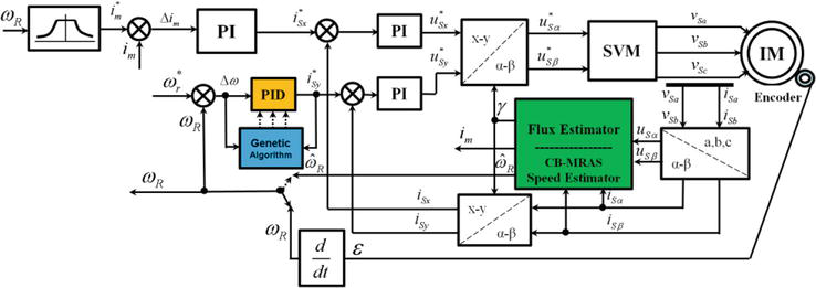
From the above equation system, vector-controlled structure of induction motor is established as follows (Figure 1).

Figure 1.

The FOC speed control structure of the induction motor drive.

2.2 Traditional PID speed controller

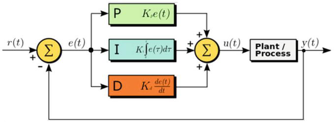
The feature of the PID controller is the ability to use the three control terms of proportional, integral, and derivative influence on the controller output to apply precise control (see Figure 2).

Figure 2.

The block diagram of the PID control.

From the above diagram, the classical PID speed controller for the induction motor drive can be expressed as follows:

$$i_{q\_\mathit{ref}}=K_p\left({\omega }_{m\_\mathit{ref}}-{\omega }_m\right)+K_i\int \left({\omega }_{m\_\mathit{ref}}-{\omega }_m\right)\mathit{dt}+K_d\frac{d\left({\omega }_{m\_\mathit{ref}}-{\omega }_m\right)}{\mathit{dt}}$$E15

The i_{q_ref} is the torque generating component called the reference current, the actual angular speed of the rotor is ω_m, the reference angular speed is ω_{m_ref}, K_p is the scaling factor, K_i is the integral factor, and K_d is the differential coefficient.

The actual value is compared with the reference value, and this deviation e_ω is handled by the PID speed controller. These parameters determine the characteristics of the electrical equipment [4, 5].

When starting the control cycle, normally the PID controller has a large scaling factor K_p to increase and decrease the speed quickly, the integral coefficient K_i must be small, and the differential coefficient K_d must be large to avoid overshoot. When the motor reaches the desired value, the scaling factor is small, the integral factor is large, and the differential factor is small to stabilize the motor speed at the reference value. The value of K_p is changed between K_pmin and K_pmax, K_i is changed between K_imin and K_imax, and K_d is changed between K_dmin and K_dmax to achieve satisfactory control performance.

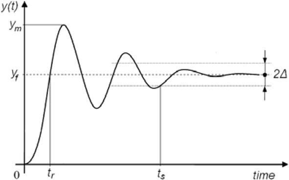
The quality of the controller is evaluated according to the input parameters of the control loop as shown in Figure 3. The evaluation factors are t_r (the t_r is rise time), t_s (the t_s steady time), y_m (the y_m is overshoot), and Δ (the Δ is steady state error) [4].

Figure 3.

The standard feedback for the control structure.

2.3 The intelligent algorithms

2.3.1 The genetic algorithm

This part will present the GA algorithm, how to determine cost function, a diagram of the GA-PID block in Matlab Simulink as well as details to implement algorithms for a speed-controlled structure of induction motor with a sensorless field-oriented model.

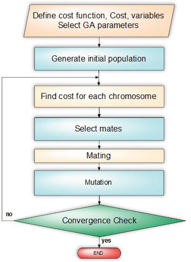
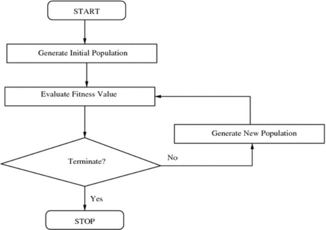
In this section, we will find the optimal parameters K_p, K_i, and K_d for PID controller by real number GA algorithm with the flowchart as follows (Figure 4):

Figure 4.

The flowchart of the genetic algorithm.

2.3.2 The particle swam optimization (PSO) algorithm

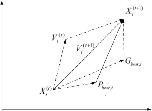
The particle swam optimization algorithm is an optimization technique. It simulates the foraging of a school of fish or a flock of birds in nature [6, 7]. Simplicity, stable convergence, good computational efficiency, etc., are the advantages of this algorithm. Optimization problems often use this algorithm, such as adjusting the gain of the controller, recognizing parameters [3], and reducing losses in the power system [12]. With the PSO algorithm, the fish is considered a seed and forms a swarm. Each particle designates a membership outcome for the problem. Particles change their location by moving to the multidimensional search space. During the operation, each member changes its position according to the previous optimal position of each individual called P_best, and the overall optimal position called G_best as displayed in Figure 5.

Figure 5.

Image of modifying velocity and particle location of the PSO process.

In each step, the correction for the velocity and position of each individual is determined by using the current velocity and the space from Pbest to Gbest, as shown in Eqs. (16) and (17):

$$v_{\mathit{ij}}={\mathit{wv}}_{\mathit{ij}}+c_1{r}_1\left({\mathit{\text{Pbest}}}_{\mathit{ij}}-x_{\mathit{ij}}\right)+c_2{r}_2\left(\mathit{\text{Gbest}}-x_{\mathit{ij}}\right)$$E16

$$x_{\mathit{ij}}=v_{\mathit{ij}}+x_{\mathit{ij}}$$E17

$$\text{with}w=w_{\max }-\frac{\mathit{\text{iter}}}{max\mathit{\text{iter}}}\left(w_{\max }-w_{\min }\right)$$E18

Here, i: represents each individual, x_i: location of each i^th individual, v_i: speed of i^th individual, w: inaction function, c_1,2: acceleration coefficient (confident rate), and rand_1,2: a chance number over an interim [0,1], Pbest_i is the best location created by the i^th instance (best component), Gbest_i: best location created by flock (total best), last weightiness w_max, initial weightiness w_min, maximum number of iterations: maxiter, and current number of iterations: iter.

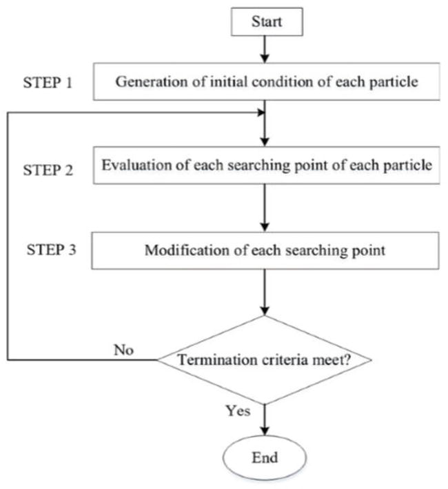
In Figure 6, the important phases in the progression of the PSO algorithm are shown below:

Figure 6.

Phases in the PSO procedure.

Step 1: Create a population of individuals whose position and speed are random in the d-dimensionality of the problematic universe within the allowed array.

Step 2: Calculate the cost function of each individual in the herd. If the present cost is better than the earlier Pbest, then Pbest is changed with the value of the present instance. If the previous value of Gbest is inferior to the best Pbest, then the value of Pbest will replace the value of Gbest and the position of the element with the most optimal value will be remembered.

Step 3: Transform the score found of each individual according to expression (17).

Step 4: Check the loop termination condition to control if it has been met (based on the cost function significance or the number of loops), if not, repeat the process from step 2. Else, the process is stopped.

2.3.3 The CSA algorithm (cuckoo search algorithm)

The key phases for CSA algorithm are shown below [8]:

1. Initialization: An inhabitant of host shells is represented by X = [X₁, X₂, …, X_Np]^T, here each shell X_d = [P_d1, …,P_dN]; d = 1,…, Np expressive in place of the parameters, these parameters are initialized by:

   $$P_{\mathit{di}}=p_{imin}+{{\mathit{rand}}_1}^{\ast }\left(p_{imax}-p_{imin}\right);i=1,\dots ,N$$E19

   where rand is a distributed random number in [0, 1] for each population of host nests. The maximum and minimum of the parameters are defined as the P_imin and P_imax.

   The establishment residents of the host shells have the greatest significance of each shell Xbest_d (d = 1,…,N_d) and the shell matches the greatest objective function and has the greatest shell Gbest among all the shells in resident.

2. Creation of new result by Lévy flights: The novel result of each shell is produced below:

   $$X_d^{\mathit{new}}={\mathit{\text{Xbest}}}_d+{\alpha }^{\ast }{{\mathit{rand}}_2}^{\ast }\mathrm{\Delta }{X}_d^{\mathit{new}}$$E20

   The objective function will be reexamined to find the new greatest value of each shell Xbest_d and the best of all shells Gbest by linking the stored calculated value and the new calculated value created.

3. Strange egg detection and randomization

   A strange egg in the shell of a host bird with probability P_a is detected. A new result similar to Lévy flights generated by this event is shown below:

   $$X_d^{\mathit{dis}}={\mathit{\text{Xbest}}}_d+K^{\ast }\mathrm{\Delta }{X}_d^{\mathit{dis}}$$E21

   Here, K is the coefficient updated and determined based on the probability that the host bird detects an alien egg in their shell.

   $$\begin{array}{l}\mathit{\text{if}}{\mathit{rand}}_3<p_a\mathit{\text{then}}K=1\mathit{\text{else}}K=0\\ \mathrm{\Delta }{X}_d^{\mathit{dis}}={{\mathit{rand}}_4}^{\ast }\left({\mathit{\text{randp}}}_1\left({\mathit{\text{Xbest}}}_d\right)-{\mathit{\text{randp}}}_3\left({\mathit{\text{Xbest}}}_d\right)\right)\end{array}$$E22

   Like the result of Lévy flights, this novel result is also resolute again for each shell Xbest_d and the greatest importance of all shells Gbest is established based on significance acquired from (21).

4. Stopping conditions: The CSA algorithm is finished when the recent repetition is like or larger than the maximum number of repetitions (Figure 7).

Figure 7.

Steps in CSA algorithm.

2.4 The speed controller of IM using genetic algorithm

To perform a genetic algorithm as well as some other soft computing algorithms, it is very important to find the cost function correctly, below is how to define it.

From equation in the continuous time:

$$u\left(t\right)=K_{p}e\left(t\right)+K_i\underset{0}{\overset{t}{\int }}e\left(t\right)\mathit{dt}+K_{d}e\left(t\right)$$E23

To determine the objective function, the moment-generating component is represented in the discrete form with the sampling cycle ΔT as shown below:

$$\underset{0}{\overset{t_k}{\int }}e\left(\tau \right)\mathit{d\tau }=\sum _{i=1}^{k}e\left(t_i\right)\mathrm{\Delta }t$$E24

and

$$\frac{\mathit{de}\left(t_k\right)}{\mathit{dt}}=\frac{e\left(t_k\right)-e\left(t_{k-1}\right)}{\mathrm{\Delta }t}$$E25

Here, the endless time inaccuracy at the i^th sampling time is e(t_i). Then, the expression becomes:

$$u\left(t_k\right)=K_p(e\left(t_k\right)+\frac{\mathrm{\Delta }t}{T_i}\sum _{i=1}^{k}e\left(t_i\right)+\frac{T_d}{\mathrm{\Delta }t}\left(\mathrm{e}\left({\mathrm{t}}_k\right)-\mathrm{e}\left({\mathrm{t}}_{k-1}\right)\right)$$E26

The u(t_k) can also be calculated from u(t_k-1) as follows:

$$\begin{array}{l}u\left(t_k\right)=u\left(t_{k-1}\right)+K_p\left(1+\frac{\mathrm{\Delta }t}{T_i}+\frac{T_d}{\mathrm{\Delta }t}\right)(e\left(t_k\right)\\ +K_p\left(-1-\frac{2T_d}{\mathrm{\Delta }t}\right)\mathrm{e}\left({\mathrm{t}}_{k-1}\right)+K_p\frac{T_d}{\mathrm{\Delta }t}e\left(t_{k-2}\right)\end{array}$$E27

$$\text{with}:K_i=T_i/K_p;K_d=K_p{T}_d$$

$$e_k={\omega }_{m\_\mathit{ref}\left(k\right)}-{\omega }_{m\left(k\right)}$$

$$u\left(t_k\right)-u\left(t_{k-1}\right)={\mathrm{\Delta }}_{\mathit{sy}\_\mathit{ref}}=i_{\mathit{sy}\_\mathit{ref}\left(k\right)}-i_{\mathit{sy}\_\mathit{ref}\left(k-1\right)}$$

Eq. (27) is rewritten as shown below:

$${i_{\mathit{sy}\_\mathit{ref}}}_k^{}={i_{\mathit{sy}\_\mathit{ref}}}_{k-1}^{}+K_p\left(1+\frac{\mathrm{\Delta }t}{T_i}+\frac{T_d}{\mathrm{\Delta }t}\right)e_k+K_p\left(-1-\frac{2T_d}{\mathrm{\Delta }t}\right)e_{k-1}+K_p\frac{T_d}{\mathrm{\Delta }t}{e}_{k-2}$$E28

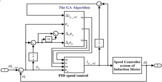
2.5 The detail block and the steps to implement GA-PID speed controller

From this expression, the designed schematic of GA-PID block is as below (Figure 8).

Figure 8.

The speed controller using genetic algorithm.

The right-hand side of expression (28) will be evaluated to collect the new values of the K_p, K_i, and K_d. All parameters in the overhead equation, except ${i_{\mathit{sy}\_\mathit{ref}}}_k^{}$, are known at the (k−1)^th sampling point. If the different values of K_p, K_i, and K_d are chosen, then obviously the different reactions of the plant will be collected. Therefore, the parameter adjustment problem of the PID controller can be considered by choosing the three parameters K_p, K_i, and K_d, so that the response of the plant will be as desired to automatically detect PID parameter online.

2.6 Simulation results

The Matlab Simulink is used to simulate the controller of an induction motor with the following parameters: P = 1HP, U_dc = 300 V, P_p = 2, R_S = 2.1 Ω, R_r = 1.51 Ω, L_m = 0.129H, J = 0.043 Kg.m², and L_S = 0.137 H. The list of control parameters is given in Table 1.

Parameter	GA speed controller	Classical PI controller
Proportionate coefficient Kp	[0–50] A/rad/s	90 A/rad/s
Integral coefficient Ki	[0–50] A/rad	90 A/rad
Derivative coefficient Kd	[0–50] A/rad.s^2	2A/rad.s^2
Generations number (i)	3
The coefficients Kp, Ki, and Kd in populace (j)	8

Table 1.

The speedy control has the based parameters as below.

Figures 9–16 display important characteristics of speed controller of the induction motor under different operating conditions.

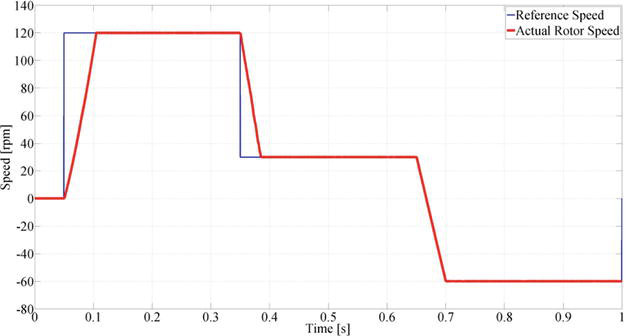
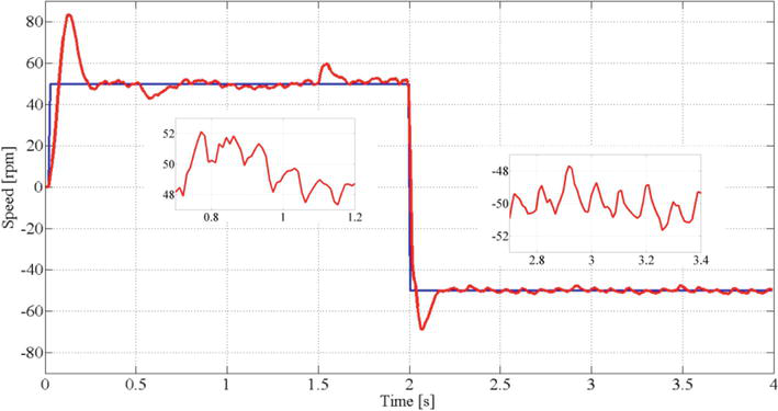
Figure 9.

Reference speed ω_{m_ref} (blue) and actual rotor speed ω_m (red) of the IM with traditional PID speed controller without load.

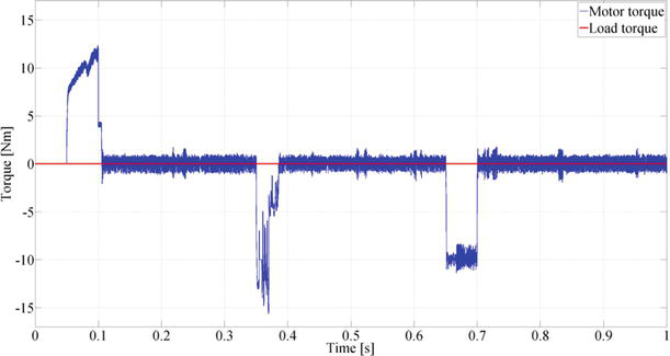
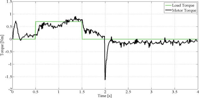
Figure 10.

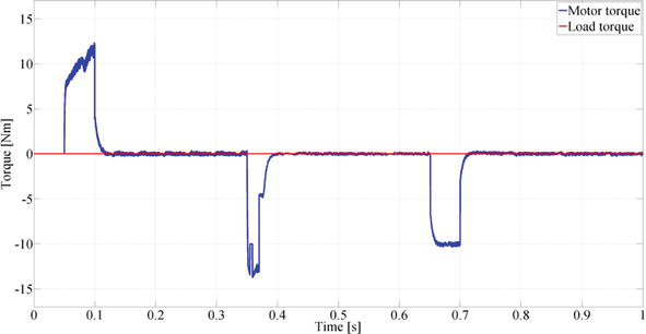
Load torque (red) and induction motor torque (blue) with traditional PID speed controller.

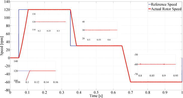
Figure 11.

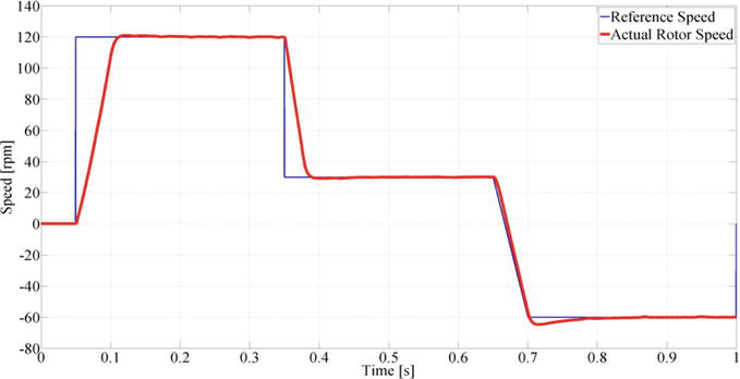
Reference speed ω_{m_ref} (blue) and actual rotor speed ω_m (red) of the IM with traditional PID speed controller has the load.

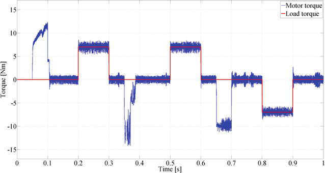
Figure 12.

Load torque (red) and induction motor torque (blue) with traditional PID speed controller.

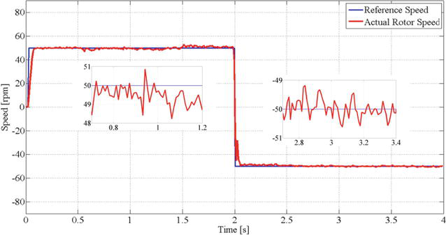
Figure 13.

Reference speed ω_{m_ref} (blue) and actual rotor speed ω_m (red) of the IM with the online PID speedy control using the GA algorithm without load.

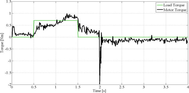
Figure 14.

Load torque (red) and induction motor torque (blue) with the online PID speedy control using the GA algorithm.

Figure 15.

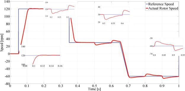
Reference speed ω_{m_ref} (blue) and actual rotor speed ω_m (red) of the IM with the online PID speedy control using the GA algorithm has the load.

Figure 16.

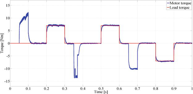
Load torque (red) and induction motor torque (blue) with the online PID speedy control using the GA algorithm.

2.6.1 Traditional PID speed controller

2.6.1.1 Traditional PID speed controller without load

Under the no-load condition, the speed response of the PID controller for the induction motor is quite good (see Figure 9).

Figure 10 shows the load torque and induction motor torque.

2.6.1.2 Traditional PID speed controller with load

For a traditional PID speedy control in case of load, the speed response varies quite a lot.

2.6.2 The online PID speedy control using the GA algorithm

2.6.2.1 The online PID speedy control using the GA without load

With the PID speedy control using the GA algorithm to optimize the parameters K_p, K_i, and K_d, in the case of no load or load, the speed response is still stable (see Figures 13 and 15).

2.7 Experimental results

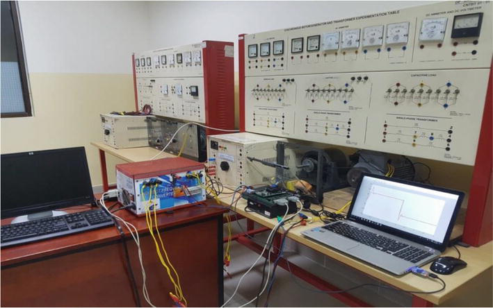
This experiment was performed in the laboratory. Our experimental model is shown below, the equipment includes the TMS 320F82335 board, the inverter with the Semikron IGBT, the drive supply modulated voltage for the induction motor, 3-phase induction motor, the generator load for a motor, 3-phase transformer output voltage varies from 0–220 Vac. We did experiment for both control methods above such as the simulation part at different speed in two cases no-load and load. The figure below shows the results (Figure 17).

Figure 17.

The DSP-28335 board and IM motor used in experiment.

2.7.1 The traditional PID speed control without load

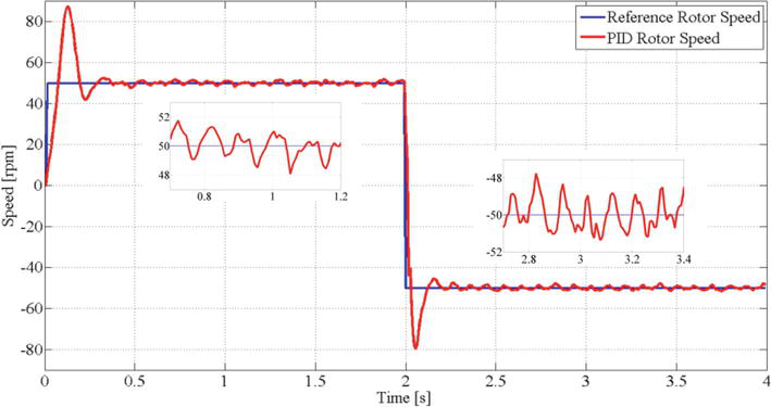
In actual performance, the traditional PID speed controller has a rather large overshoot compared to the PID using the genetic algorithm (see Figure 18).

Figure 18.

Real rotor speed ω_m (red) and mention speed ω_{m_ref} (blue) of the induction motor.

2.7.2 The online GA-PID speed control without load

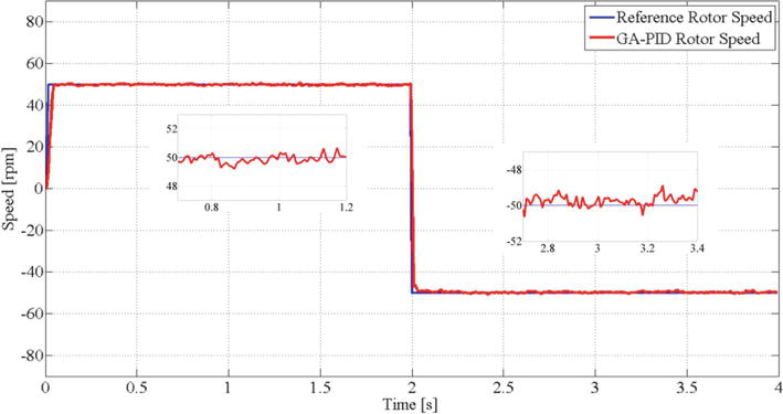
In the experiment with the PID speed controller using a genetic algorithm to optimize control parameters, the speed response is still stable in the no-load case (see Figure 19).

Figure 19.

Reference speed ω_{m_ref} (blue) and actual rotor speed ω_m (red) of the IM in the online GA-PID speed control without load.

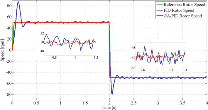
Compare the speed response of the two methods on the same coordinate system without load (see Figure 20).

Figure 20.

Real rotor speed ω_m (red) and desired speed ω_{m_ref} (blue) of the IM in the above two methods without load.

2.7.3 The traditional PID speed control with load

Figures 21 and 22 show the speed and torque response of the IM according to the traditional PID control model. The speed response of an induction motor applying the online genetic algorithm remains stable under load (see Figure 23).

Figure 21.

Reference speed ω_{m_ref} (blue) and actual rotor speed ω_m (red) of the IM in the traditional PID speed control with load.

Figure 22.

The load torque (green) and IM torque (black) of the PID speed controller with load.

Figure 23.

Reference speed ω_{m_ref} (blue) and actual rotor speed ω_m (red) of the IM in the online GA-PID speed control with load.

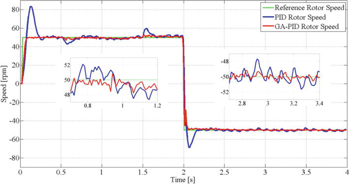
Figure 24 depicts the load torque and IM torque in the online GA-PID speed control with the load. The comparison of the speed response with the load of the IM between the traditional PID controller and the online GA-PID controller is shown in Figure 25.

Figure 24.

Load torque (green) and IM torque (black) of in the online GA-PID speed control with load.

Figure 25.

Reference speed ω_{m_ref} (green), PID rotor speed of the IM ω_est (blue), and GA-PID rotor speed ω_m (red) of the IM with load.

2.7.4 The online GA-PID speed control with load

3. Conclusion

This chapter presented some intelligent algorithms such as GA, PSO, and CSA algorithms to apply to the control model of induction motors. In the paper, the application of the GA algorithm in the speed control of induction motors has been presented in detail. The speed control of the induction motor by conventional PID in case of no-load or unchanged working conditions is quite good, but under variable conditions, the control quality is not guaranteed. In the case of speed control of induction motor using PID controller where the optimal proportional parameter K_p, integral K_i, and differential K_d are updated continuously by genetic algorithm, the speed response is very good and stable under load or no-load conditions. These have been proven through simulation results on Matlab Simulink as well as in experiment with TI’s DSP-28335 board above.

In the content of this topic, having mentioned the speed control for induction motors by field-oriented method, readers can apply the algorithms mentioned in the torque control model for IM motors or search motor parameters such as stator resistance, rotor, stator winding inductance, rotor, and rotor time constant (because the quality of IM motor control according to torque model or field orientation depends heavily on the parameters of IM motor).

In addition, other motors such as PMSM motors and Brushless DC motors are also widely applied in the field of industrial robots, machines with high precision control needs, due to strong torque and higher working efficiency than induction motor. Therefore, the application of the presented algorithms: GA, PSO, CSA algorithm, etc., to the optimal control of these motors (PMSM motor, Brushless DC motor, etc.) as well as develop more algorithms and other smarts such as Artificial Neural Network (ANN), Fuzzy, sliding mode control, extended Kalman filter (EKF), or a combination of these algorithms will contribute to bringing good efficiency to our industry and lives.

References

1.Vas P. Vector Control of AC Machines. Oxford: Clarendon Press; 1990
2.Vas P. Artificial-intelligence-based electrical machines and drives: application of fuzzy, neural, fuzzy-neural, and genetic-algorithm-based techniques. Oxford University Press; 1999
3.Banerjee T, Sumana C, Jitendranath B, Abhisek M, et al. Off-line optimization of PI and PID controller for a vector controlled induction motor drive using PSO. In: Proceedings of International Conference on Electrical & Computer Engineering (ICECE). IEEE. 2010. pp. 74-77. DOI: 10.1109/ICELCE.2010.5700556
4.Tran TC, Brandstetter P, Duy VH, Vo HH, Dong C. PID speed controller optimization using online genetic algorithm for induction motor drive. In: International Conference on Advanced Engineering Theory and Applications. Cham: Springer; 2016. pp. 564-576. DOI: 10.1007/978-3-319-50904-4_60
5.Laroussi K, Zelmat M, Rouff M. Implementation of a fuzzy logic system to tune a PI controller applied to an induction motor. Advances in Electrical and Computer Engineering. 2009;9(3):107-113. DOI: 10.4316/AECE.2009.03019
6.Rekha M, Kumar MK. Variable frequency drive optimization using torque ripple control and self-tuning PI controller with PSO. International Journal of Electrical and Computer Engineering (IJECE). 2019;9(2):802-814. DOI: 10.11591/ijece.v9i2.pp802-814
7.Dang HS, Palacky P, Kuchar M, Brandstetter P, Tran CD. Particle swarm optimization-based stator resistance observer for speed sensorless induction motor drive. International Journal of Electrical and Computer Engineering. 2021;11(1):815. DOI: 10.11591/ijece.v11i1.pp. 815-826
8.Hassan AY, El-latifBadr MA, Wahsh SA E-m. Cuckoo search based real time implementation of direct torque control of PMSM. In the 2018 Twentieth International Middle East Power Systems Conference (MEPCON). IEEE; 2018. pp. 235-241. DOI: 10.1109/MEPCON.2018.8635189
9.Kennedy J, Eberhart R. Particle swarm optimization. In: Proceedings of ICNN’95-international conference on neural networks; 1995. IEEE. vol. 4, pp. 1942-1948. DOI: 10.1109/57ICNN.1995.488968
10.Shi Y, Eberhart R. A modified particle swarm optimizer. In: Proceedings of the IEEE International Conference on Evolutionary Computation. IEEE. 1998. pp. 69-73. DOI: 10.1109/ICEC.1998.699146
11.Karanayil B et al. Online stator and rotor resistance estimation scheme using artificial neural networks for vector controlled speed sensorless induction motor drive. IEEE Transactions on Industrial Electronics. 2007;54(1):167-176. DOI: 10.1109/TIE.2006.888778. DOI: 10.1109/ICELCE.2010.5700556
12.Tofighi EM, Mahdizadeh A, Feyzi MR. Online estimation of induction motor parameters using a modified particle swarm optimization technique. In: Proceedings of IECON 2013-39th Annual Conference of the IEEE Industrial Electronics Society. IEEE. 2013. pp. 3645-3650. DOI: 10.1109/IECON.2013.6699715
13.Mini R, Shabana Backer P, Satheesh H, M. N. Dinesh: Low speed estimation of sensorless DTC induction motor drive using MRAS with neuro fuzzy adaptive controller. International Journal of Electrical and Computer Engineering (IJECE). 2018;8(5):2691-2702. DOI: 10.11591/ijece.v8i5.pp2691-2702
14.Sreejeth M, Singh M, Kumar P. Efficiency enhancement for indirect vector-controlled induction motor drive. International Journal of Electronics. 2019;106(9):1281-1294. DOI: doi.org/10.1080/00207217.2019.1584921
15.Girovsky P, Timko J, Zilkova J. Shaft sensor-less FOC control of an induction motor using neural estimators. Acta Polytechnica Hungarica. 2012;9(4):31-45
16.Karanayil B et al. Stator and rotor resistance observers for induction motor drive using fuzzy logic and artificial neural networks. IEEE Transactions on Energy Conversion. 2005;20(4):771-780. DOI: 10.1109/TEC.2005.853761
17.Vasic V et al. A stator resistance estimation scheme for speed sensorless rotor flux oriented induction motor drives. IEEE Transactions on Energy Conversion. 2003;18(4):476-483. DOI: 10.1109/TEC.2003.816595
Written By
Thinh Cong Tran, Pavel Brandstetter and Martin Kuchar
Submitted: 22 February 2023Reviewed: 09 April 2023Published: 06 July 2023
Open access peer-reviewed chapter