Markov Models Related to Inventory Systems, Control Charts, and Forecasting Methods

Abstract

A Markov model describes a randomly varying system that satisfies the Markov property. This means that future and past states at any time are independent of the current state. The two most commonly used types of Markov models are Markov chains and higher-order Markov chains. Therefore, three types of Markov models are proposed in this chapter of the book: (i) supply chain management, (ii) Markov queue waiting time monitoring, and (iii) Markov fuzzy time series forecasting. The introduction introduces Markov chain (MC) and summarizes the most important aspects of Markov chain analysis. The first model explores a Markov queue model coupled to a storage system using the classical (0, Q) policy. The second model focuses on the M/M/1/N service mode and develops a control chart for an M_s/M_s/1/N type simulated queue to monitor customer waiting times. The third is a higher-order Markov model (HOMM), which uses fuzzy sets to predict future states based on given hypothetical time series data. Numerical calculations are designed to find optimal order quantities, monitor customer wait times, and predict future HOMM conditions.

1. Introduction

The term probability refers to the proportion of interesting events observed in one or more random experiments. The probability of an event A occurring in an experiment is given by the ratio f/T, where f = A can occur and T = the total number of possible outcomes of this experiment. We denote the set of all outcomes of a random experiment by Ω = {ω}, which is called the sample space. A real-valued function X = X(ω) that gives a unique real value for each term “ω” in the real set R (= (−∞, ∞)) is called a (real valued) random variable. We classify a random variable as discrete if it has only a few specific values, such as −1, 3, 8, and 17. Otherwise, it is classified as continuous. A family of random variables indexed by time “t” defined on a state space $\mathbb{S}$ i.e., $\mathrm{X}=\left\{\mathrm{X}\left(\mathrm{t}\right)\in \mathbb{S}:\mathrm{t}\in \mathrm{T}=\left[0,\infty \right)\right\}$ is called a stochastic process. Thus, a typical Stochastic process is indexed by time “t” and takes its state values over a space $\mathbb{S}$ is represented as

$$X=\left\{X\left(\omega ,t\right)\in \mathbb{S},\omega \in \mathrm{\Omega },t\in T\right\}$$E1

1.1 Continuous time (CT) Markov process (MP) {X(t), t > 0}

If the probability of future state of X(t) depends only on the present but not on the past states then {X(t), t > 0} is a MP for any set of time points $t_1<t_2<\cdots <t_{n+1}$ and any set of states $x_1<x_2<\cdots <x_{n+1}\Rightarrow$

$$\begin{array}{l}Pr\left(X\left(t_{n+1}\right)=\left.x_{n+1}\right|X\left(t_1\right)=x_1,X\left(t_2\right)=x_2,\dots ,X\left(t_n\right)=x_n\right)=\\ Pr\left(X\left(t_{n+1}\right)=\left.x_{n+1}\right|X\left(t_n\right)=x_n\right).\end{array}$$E2

1.2 Markov Chain {X_n: n = 0,1 2,…}

• A discrete time MP {X_t = X_n: n = 0,1 2,…} is called a Markov chain (MC). Let the conditional probability of moving from state i to state j be P_ij = P(X_(n + 1) = j | X_n = i), n ≥ 0 and i, and j = 0,1,2,….

• Define one step transition probability matrix (TPM): $\mathbb{P}=\left[P_{\mathit{ij}}\right]$ Let $P_{\mathit{ij}}^m=$. The conditional probability of moving to state j starting from state i in m steps which can be calculated using the Chapman Kolmogorov (CK) equations:

  $$P_{\mathit{ij}}^m=Pr\left(\left.X_m=j\right|X_0=i\right)=\sum _{k=0}^{\infty }{P}_{\mathit{ik}}^r{P}_{\mathit{kj}}^{m-r}$$E3
  $$\text{for}i,j=0,1,2,\dots \text{and}m\ge r\ge 0.$$E4

• Thus, the m^th step TPM is ${\mathbb{P}}^m=\left[P_{\mathit{ij}}^m\right]$.

• A MC is completely determined if the initial distribution P(X₀ = j) and its one step TPM P are all known or estimated by conducting a sample survey.

1.3 Classification of States of a MC

• State j is accessible from state i if there exists an integer m such that $P_{\mathit{ij}}^m>0$.

• Two states i and j communicate with each other if both are accessible from each other.

• The TPM of an MC defined on a state space $\mathbb{S}$ is said to be irreducible if all states communicate with each other state in $\mathbb{S}$.

• State i is recurrent if the system will return to it after some finite time in the future.

• If a state is not recurrent, it is transient.

• A state is periodic if it can only return to itself after a fixed number of transitions greater than 1 (or multiple of a fixed number).

• A state that is not periodic is aperiodic.

• An absorbing state is one that locks in the system once it enters.

• All states belonging to a class are either recurrent or all transient and may be either all periodic or aperiodic.

1.4 Stationary distribution of an aperiodic and irreducible MC

• Let and

  $${\pi }_j=\underset{n\to \infty }{lim}{P}_{\mathit{ij}}^n\text{and}\mathrm{\Pi }=\left\{{\pi }_0,{\pi }_1,{\pi }_2,\dots \right\},{\sum }_{j=0}^{\infty }{\pi }_j=1.$$E5

• Under certain conditions, these limiting probabilities π_j can be shown to exist and are independent of the starting state i.

• They represent the long run proportions of time that the process spends in each state j. Also π_j = the steady-state probability that the process will be found in each state j. Computation of the row vector Π:

  $$\mathrm{\Pi }\mathbb{P}=\mathrm{\Pi },\sum _{j=0}^{\infty }{\pi }_j=1.$$E6

• For an aperiodic and recurrent MC on the state space Ω = {1, 2,…,m}. Let ${\pi }_j=\underset{n\to \infty }{lim}{P}_{\mathit{ij}}^n$, ${\sum }_{j=0}^m{\pi }_j=1$ and row vector Π = (π₀, π₁,…, π_m).

• Then, the stationary probability vector Π satisfies the following set of simultaneous equations:

  $$\mathrm{\Pi }\mathbb{P}=\mathrm{\Pi },\mathrm{\Pi }\mathbf{1}=1=\sum _{j=0}^m{\pi }_j$$E7

• Computational Hint: One of the m equations of $\mathrm{\Pi }\mathbb{P}=\mathrm{\Pi }$ is redundant. It is advised that replacing any of the equations of Π P = Π by Π 1 = 1, we form a set of m simultaneous equations which yield the unique Π. One can find quite a number of applications of finite state MCs in our social life activities.

1.5 Generator Matrix of a continuous time MP

Let T_ij denote the time for the MP to go from state i to state j and q_ij be the known rate of transition from state i to state j.

Then $T_{\mathit{ij}}\to e^{q_{\mathit{ij}}}$. Let q_i = ∑_j ≠ iq_ij,

The infinitesimal generator is

$$Q=\left[\begin{array}{ccccc}-q_0& q_{01}& q_{02}& q_{03}& \dots \\ q_{10}& -q_2& q_{12}& q_{13}& \dots \\ q_{20}& q_{21}& -q_3& q_{23}& \dots \\ ⋮& ⋮& ⋮& ⋮& ⋮\end{array}\right]$$E8

The stationary distribution is obtained by solving the system of equations

$$\mathrm{\Pi }Q=\mathbf{0},\mathrm{\Pi }\mathbf{1}=1=\sum _{n=0}^{\infty }\pi$$E9

Basic information on MC definition, classification of states, etc. can be found in [1, 2]. Instructions for calculating the state characteristics of different types of MCs using software “markov chains” are briefly discussed in [3].

1.6 Ordering Markov models discussed

Section 2 considers customer arrivals to demand a single product of supply chain management. All arrivals join an M/M/1/N/FCFS system attached to a storage house under the classical (0, Q) policy. The joint process of limiting queue length and the inventory level is denoted by Z = {(L, J)} = lim_t → ∞{(L(t), J(t))}. We then obtain stationary probability vector of the Z process. A cost function is formed as an implicit function of the order quantity Q and other input values, and the optimal order quantity that minimizes its total cost is determined.

Section 3 presents the analysis on an M/M/1/N queue and develops simulated queue M_s/M_s/1/N. The steady state characteristics such as the embedded queue length and waiting times at all successive transition epochs of the M_s/M_s/1/N system are obtained and a control chart is constructed to monitor the impacts of the customer’s waiting time distribution.

Section 4 introduces a HOMM for analyzing a fuzzy time series as a data sequence. The main focus is to build a first-order MC (FOMC) and another second-order MC (SOMC) for the same data sequence under study. The prediction error (PE) is calculated for both FOMC and SOMC and a comparison is made to isolate the best performer. Section 5 provides a formal concluding report.

2. Markov model for supply chain managements

A Markov chain sequence can be thought of as a stochastic model. Such a model involves mathematical considerations to estimate the probability of a sequence of future states based on the most recent event rather than past history. The Markov model is a stochastic method for randomly varying systems with the Markov property. This means that at any moment the next state depends only on the current state and is independent of the past.

Markov analysis is a method for predicting the value of a variable whose predicted value is affected only by its current state and not by any past activity. Basically, it predicts a random variable based only on current conditions. The three simple forms of Markov models are (i) MC, (ii) Markov decision process (MDP), and (iii) HOMM. Each model has applications in queuing theory, inventory systems, and reliability theory.

To learn the analysis of queuing problems, researchers can read [1, 2, 4, 5, 6, 7, 8, 9]. Regarding stochastic model building using queuing storage systems, you can refer to [8, 10, 11, 12]. The use of matrix analysis to find steady state results for queue-length processes is well covered in the book by [13].

2.1 Markov decision processes of a supply chain

Supply chain (SC) is a system that links sales branches into a supply chain that would financially improve customer satisfaction and loyalty. Several SC researchers have used integrated queues with inventory policies to reduce lead time and inventory costs.

This section discusses a Markov model that tracks inventory levels in a warehouse connected to a queuing system that sells individual products based on customer demand. This is called the Queue inventory model (QIM), which allows demands to be made during the inventory period. However, those customers who arrive when the warehouse is empty will not be processed until after the ordered products arrive.

The proposed SC facility delivers either a package of Q > 0 fixed-size items for the normal order or only one item for an emergency order to a warehouse that processes customer requirements through a Markov service node M/M/1/N.

Denoting the number of customer demands occurred at time “t” by X(t) and the present on-hand inventory level by Y(t), we propose matrix methods to study the bi-variate stochastic process Z(t) = (X(t), Y(t)) defined on the state space E = N₀xQ₀ where N₀ = 0, 1, 2, …, N and Q₀ = 0, 1, 2, …, Q. The system has a single server who admits a maximum number “N” of customers and does not admit those customers who arrive at instances when X(t) = N called lost customers. The queue discipline is on a first-come, first-served basis (FCFS).

Customers requesting one unit of stock arrive at a node of a Poisson process with mean parameter (λ) when X(t) = n, nge0. For each request, after an exponential service time, one product unit is offered with a state-dependent parameter μ_n. Here we have two types of inventory ordering policies called “regular” and “emergency”:

1. The normal ordering is the classical (0, Q(>1)) policy, which is set whenever the MDP Z(t) moves from (n,0) to (n + 1,1) n ≥ 1. The lead time is assumed to be an exponentially and identically distributed random variable with rate parameter γ.

2. The emergency ordering type is the classical (0, Q(=1)), which triggers an order for one product whenever the Z(t) process moves from (1,1) to (0,0). It is assumed that the emergency fulfillment time is a small interval of unit length (IUL) and the urgent order is replenished at a rate of “1.” This emergency order period expires at the end of the IUL. In this particular period, P[(0,0) → (0,1)] = 1/(λ + 1), P[(0,0) → (1,0)] = λ/(λ + 1), that is, whether the replenishment of one product or the arrival of a customer demand is unavoidable.

3. Our M/M/1/N service system will not accept every incoming customer if there are N customers in front of the system. There can be at most one pending order where “0” is the order point and the order quantity is at most Q units per replenishment for the normal type and only one product for the emergency type.

Due to the properties of exponential distributions and the mixed-type of normal and emergency practices, the proposed sequence Z(t) forms an aperiodic and positive recurrent Markov decision process (MDP). The set properties of the Z system can be easily checked at each stage of service completion. Our main objective is to use a linear function of expected total cost to determine the optimal order quantity and order patterns.

2.2 Generator matrix of the MDP process Z

It is interesting to note that the MDP process Z is also a level-dependent quasi-birth-and-death (LDQBD) in continuous time. We have the (N + 1) level L_n such that ${\bigcup }_{n=0}^N{L}_n=\mathrm{E}$. The infinitesimal generator matrix G has the tri-diagonal structure and each submatrix of G is a square matrix of order (Q + 1):

$$\mathbf{G}=\left[\begin{array}{ccccccc}\mathrm{B}& {\mathbf{A}}_0& 0& 0& \dots & \mathbf{0}& \mathbf{0}\\ {\mathrm{A}}_2& {\mathrm{A}}_{\mathbf{1}}& {\mathbf{A}}_{\mathbf{0}}& 0& \dots & \mathbf{0}& \mathbf{0}\\ 0& {\mathrm{A}}_2& {\mathrm{A}}_{\mathbf{1}}& {\mathbf{A}}_{\mathbf{0}}& \dots & \mathbf{0}& \mathbf{0}\\ 0& 0& {\mathrm{A}}_2& {\mathrm{A}}_{\mathbf{1}}& \ddots & \mathbf{0}& \mathbf{0}\\ ⋮& ⋮& ⋮& \ddots & \ddots & {\mathbf{A}}_{\mathbf{0}}& \mathbf{0}\\ \mathbf{0}& \mathbf{0}& \mathbf{0}& \mathbf{0}& \ddots & {\mathrm{A}}_{\mathbf{1}}& {\mathbf{A}}_{\mathbf{0}}\\ \mathbf{0}& \mathbf{0}& \mathbf{0}& \mathbf{0}& \dots & {\mathrm{A}}_2& \left({\mathrm{A}}_1+{\mathbf{A}}_{\mathbf{0}}\right)\end{array}\right]$$E10

Each sub-matrix of the G is a square matrix of order (Q + 1) indexed by j = 0, 1, …, Q. The precise structures of B = (b_{i j}), ${\mathbf{A}}_0=\left(a_{ij}^{\left(0\right)}\right),$${\mathbf{A}}_1=\left(a_{ij}^{1)}\right),$ and ${\mathbf{A}}_2=\left(a_{ij}^{\left(2\right)}\right)$ are now described:

$$b_{ij}=\left\{\begin{array}{c}{b}_{11}=-\left(\lambda +1\right)b_{12}=1b_{1j}=0\text{for}\mathrm{j}=3,4,\dots ,\left(\mathrm{Q}+1\right)\\ b_{ij}=-\lambda \text{for}1=\mathrm{j}=2,..\left(\mathrm{Q}+1\right)\\ 0\mathit{\text{otherwise}}\end{array}\right.$$E11

$$a_{ij}^{\left(0\right)}=\left\{\begin{array}{c}\lambda \text{for}\mathrm{i}=\mathrm{j}=1,2,..\left(\mathrm{Q}+1\right)\\ 0\mathit{\text{otherwise}}\end{array}\right.$$E12

$$a_{ij}^{\left(1\right)}=\left\{\begin{array}{c}{a}_{11}^{\left(1\right)}=-\left(\lambda +\nu \right)a_{1\left(Q+1\right)}^{\left(1\right)}=\nu \\ -\left(\lambda +\mu \right)\text{for}\mathrm{i}=\mathrm{j}=2,3,\dots ,\left(\mathrm{Q}+1\right)\\ 0\mathit{\text{otherwise}}\end{array}\right.$$E13

$$a_{ij}^{\left(2\right)}=\left\{\begin{array}{c}{a}_{i\left(i-2\right)}^{\left(2\right)}=\mu \text{for}\mathrm{i}=2,\dots ,\left(\mathrm{Q}+1\right)\\ 0\mathit{\text{otherwise}}\end{array}\right.$$E14

The solution of matrix equations generated by level-dependent QBD processes has been widely studied by several researchers, see [6]. A useful matrix analysis method for computing the steady-state probability distributions of the queue-length process of QBDs is presented in Ref. [13].

Distribution: Denote by П = (π_0,π_1,π₂, …., π_N), the steady state distribution of Z and by π_n the row vector π_n = (π(n, 0), …, π(n, Q)) associated with level L_n, $n\in N_0.$ Let e = (1,1, …,1) be a column vector of unit elements.

We now discuss a simple linear level reduction method in two phases for a positive recurrent case that leads to computation of the limiting distribution П: Phase 1: Iteratively reduce the state space from the level “N” by removing one level at each step until we reach the level “0” and check if the generator of the level “0” corresponds to a Markov process.

Compute, the U⁽ⁿ⁾ matrices and the rate matrices R_n in terms of the sub-matrices of the generator G:

$${\mathrm{U}}^{\left(N\right)}=A_1^{\left(\mathrm{N}\right)}+{\mathrm{A}}_0,$$E15

$${\mathrm{U}}^{\left(n\right)}={\mathrm{A}}_1^{\left(\mathrm{n}\right)}-{\mathrm{A}}_0{\left[{\mathrm{U}}^{\left(\mathrm{n}+1\right)}\right]}^{-1}{\mathrm{A}}_2^{\left(\mathrm{n}+1\right)}\text{for}\mathrm{n}=\left(\mathrm{N}-1\right),\left(\mathrm{N}-2\right),\dots ,1$$E16

$${\mathrm{U}}^{\left(0\right)}=\mathrm{B}-{\mathrm{A}}_{\mathbf{0}}{\left[{\mathrm{U}}^{\left(\mathbf{1}\right)}\right]}^{-1}{{\mathrm{A}}_{\mathbf{2}}}^{\left(\mathbf{1}\right)}$$E17

$${\mathbf{R}}_n=-{\mathbf{A}}_0{\left[{\mathrm{U}}^{\left(n\right)}\right]}^{-1},\mathrm{n}=1,2,\dots ,\mathrm{N}$$E18

For 1 ≤ n ≤ N, the matrix U⁽ⁿ⁾ records the transition rate from level L_n to L_n before a visit to L_(n − 1). In addition, the matrix $-{\left[{\mathrm{U}}^{\left(\mathrm{n}\right)}\right]}^{-1}{\mathrm{A}}_2^{\left(\mathrm{n}\right)}$ records the first passage time probabilities from level L_n to L_n (Figure 1).

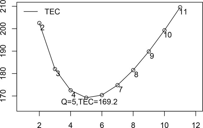
Figure 1.

Q versus TEC.

Phase 2:

Theorem 1.1 The unique stationary joint distribution vector П of the Queue length and the inventory level of the Z = (X, Y) process is given by

$${\pi }_n={\pi }_{n-1}{\mathbf{R}}_{\mathrm{n}}\mathit{\text{for}}n=1,2,\dots ,N\mathit{\text{and}}\mathbf{\Pi e}=1.$$E19

2.3 Alternative way of computing the stationary probability vector П

Phase I: Compute.

$${\mathbf{C}}_{\mathbf{0}}=\mathbf{B},{\mathbf{C}}_{\mathbf{i}}={\mathbf{A}}_{\mathbf{1}}^{\left(\mathbf{i}\right)}+{\mathbf{A}}_{\mathbf{2}}^{\left(\mathbf{i}\right)}{\left(-{\mathbf{C}}_{\mathbf{i}-\mathbf{1}}\right)}^{-\mathbf{1}}{\mathbf{A}}_{\mathbf{0}}\text{for}\mathrm{i}=1,2,\dots ,\left(\mathrm{N}-1\right),\text{and}$$E20

$${\mathbf{C}}_{\mathbf{N}}=\left({\mathbf{A}}_{\mathbf{1}}^{\left(\mathbf{N}\right)}+{\mathbf{A}}_{\mathbf{0}}\right)+{\mathbf{A}}_{\mathbf{2}}^{\left(\mathbf{N}\right)}{\left(-{\mathbf{C}}_{\left(\mathbf{N}-\mathbf{1}\right)}\right)}^{-\mathbf{1}}{\mathbf{A}}_{\mathbf{0}}$$E21

It is noticed that the matrix $\left(-{\mathbf{C}}_{\mathbf{i}}^{-\mathbf{1}}{\mathbf{A}}_{\mathbf{0}}\right)$ records the first passage probabilities from level L(i) to L(i + 1).

Phase II: The Stationary probability vector $\mathbf{\Pi }=\left({\mathbf{\Pi }}_0,{\mathbf{\Pi }}_1,{\mathbf{\Pi }}_2,\dots ,{\mathbf{\Pi }}_N\right),$${\mathrm{\Sigma }}_{n=0}^N{\mathbf{\Pi }}_{n}e=1$ is determined by

$${\mathbf{\Pi }}_N{C}_N=0,$$E22

$${\mathbf{\Pi }}_n={\mathbf{\Pi }}_{n+1}{A}_2^{\left(n+1\right)}{\left(-C_n\right)}^{-1}\text{for}\mathrm{n}=\left(\mathrm{N}‐1\right),\left(\mathrm{N}‐2\right),\dots ,3,2,1\text{and}0$$E23

2.4 Useful metrics derived from П

The marginal distribution, say П_x, of the queue length process X and that of the inventory process, say П_y are now obtained from the joint probability vector П respectively by П_x = (x₀, x₁,…, x_N) where x_n = π_ne, for n = 0,1,…, N and П_y = (y₀, y₁, …, y_Q) where $(y_j={\mathrm{\Sigma }}_{n=0}^N\pi \left(n,j\right)$ for j = 0, 1, …,Q.

Mean system Size L and Mean wait $\overline{W}$: The mean system size L and the mean sojourn time $\overline{W}$ of the queue length process X are given by

$$L=\sum _{n=0}^{N}n{\pi }_n\mathit{\text{and}}\overline{W}=\frac{L}{{\lambda }_{\mathit{eff}}},{\lambda }_{\mathit{eff}}=\lambda \left(1-{\pi }_N\right)$$E24

Mean Inventory Size $\overline{V}$ and Mean Reorder Rate $\overline{R}$: The mean inventory size $\overline{V}$ and the mean reorder rate $\overline{R}$ of the inventory level process Y are given by

$$\overline{V}=\sum _{j=0}^{Q}j{y}_j\mathit{\text{and}}\overline{R}=\mu \pi \left(1,1\right)+\sum _{n=2}^N\mu \pi \left(n,1\right)$$E25

Total expected cost (TEC) Let us consider three different costs i.e., h = holding cost per item per unit of time, c1 = ordering cost per order and c2 = waiting time cost per unit of time. A linear TEC function is then designed to determine an optimum order quantity Q^∗ for which TEC(Q^∗) is the minimum:

$$\mathit{TEC}=h\overline{V}+c1\overline{R}+c2\overline{W}$$E26

2.5 Determination of optimum order quantity, Q^∗, N = 25

A numerical representation is now considered to determine the optimal order quantity that minimizes the TEC described in (14). We set the input dataset as follows: N = 25, arrival rate λ = 2.2, service amount μ = 2.5 and replenishment rate ν = 2.25, and holding cost h = $ 27.5 order price c1 = $ 8.4, and waiting time costs c2 = $ 12.

In this case, the TEC values for varying order quantity Q are calculated with values 2 to 11, and the same is shown graphically in Figure 1. The order quantity that minimizes TEC is Q^∗ = 5 and the corresponding price is $ 169.2.

3. Markov modeling of queues with finite capacity: M/M/1/N

The chapter considers a simple simulated Markov model of a single server M/M/1/N. It focuses on a process control method that can monitor customer waiting times. Any service counter with a buffer of waiting customers naturally leads to a limited queue.

3.1 Simulation of cumulative arrival and departure epochs

The formal simulation method is now carried out to fit the M/M/1/N model, and the result is called the simulated Markov model M_s/M_s/1/N. Let the arrival rate of the M/M/1/N exponential population under investigation be λ and the service level be μ. We take enough samples from each exponential population to simulate consecutive customer arrival and departure periods, the cumulative arrival times, the number of customers in such periods, and the waiting time of each customer for a given number of arrivals such as M = 1000. The simulation process algorithm:

Step 1: Simulate “M” number of inter-arrival times {a₁, a₂, …, a_M} from the exponential distribution with parameter λ. Let the starting time of the simulation process be zero, i.e., T₀ = 0. Then calculate the sequence of cumulative arrival times T_j = T_(j − 1) + a_j for j = 1, 2, …, M.

Step 2: Simulate “M” number of service times {s₁, s₂, …, s_M} from the exponential distribution with parameter μ. Then calculate the sequence of service start time times {S_j} and the sequence of departure epochs {D_j}: S₁ = (T₁), D₁ = S₁ + s₁.

${\mathrm{S}}_{\mathsf{j}}=\mathsf{Max}\left\{\left({\mathrm{T}}_{\mathsf{j}}\right),{\mathrm{D}}_{\mathsf{j}}\right)\}\mathsf{\text{and}}{\mathrm{D}}_{\mathsf{j}}={\mathrm{S}}_{\mathsf{j}}+{\mathrm{s}}_{\mathsf{j}}\mathsf{\text{for}}\mathrm{j}=\mathsf{2},\mathsf{3},\dots ,\mathrm{M}.$

The waiting time W_j in the system for the j^th arrival is then given by W_j = D_j-T_j.

Step 3: The (pre-arrival) number ${\mathrm{L}}_j^{\left(a-\right)}$ of customers present at the arrival points {T_j} and post-departure number ${\mathrm{L}}_j^{\left(d\right)}$ of customers present at the departure points {D_j} are then calculated using appropriate formulae during the simulation period.

Step 4: If the maximum value of the sequence $\left\{{\mathrm{L}}_j^{\left(a-\right)}:\mathrm{j}=1,2,\dots ,\mathrm{M}\right\}$ is N-1, then the maximum capacity of the simulated Markov model is M_s/M_s/1/N. For cross checking, verify the fact that the maximum value of the sequence $\left\{{\mathrm{L}}_j^{\left(d\right)}:\mathrm{j}=1,2,\dots ,\mathrm{M}\right\}$ also equals to N-1.

Step 5: Let f_k = Number of times the event ${\mathrm{L}}_j^{\left(a-\right)}=\mathrm{k}$ occurred for k = 0, 1, …, (N-1) over the arrival epochs {T_j} for j = 1, 2, …, M. Then ${\mathrm{\Sigma }}_{k=0}^{\left(N-1\right)}{f}_k=\mathrm{M}$ Thus, the prearrival epoch queue length distribution is given by $\left\{{\pi }_k^{\left(a-\right)}=\frac{f_k}{M}\right\}.$.

Step 6: Let F_k = Number of times the event ${\mathrm{L}}_j^{\left(d\right)}=\mathrm{k}$ occurred for k = 0, 1, …, (N-1) over the departure epochs {D_j} for j = 1, 2, …, M, where ${\mathrm{\Sigma }}_{k=0}^{\left(N-1\right)}{F}_k=\mathrm{M}.$ Thus, the departure epoch queue length distribution is given by $\left\{{\pi }_k^{\left(d\right)}=\frac{F_k}{M}\right\}.$ For a cross-checking, verify the fact that f_k = F_k for k = 0, 1, 2, …, (N-1).

3.2 How to fit M/M/1/N

The special feature is that the maximum number “N” of the simulated version M_s/M_s/1/N plays a crucial role. Let us denote the estimated results obtained from the above simulated outcomes for pre-arrival epoch queue length probabilities by ${\pi }_j^{\left(a-\right)}$ and post-departure epoch probabilities by ${\pi }_j^{\left(d\right)}.$ Then it can be shown that

$${\pi }_j^{\left(a-\right)}={\pi }_j^{\left(d\right)};\mathrm{j}\in {\mathbb{S}}^{\left(a-\right)}=\left\{0,1,2,\dots ,\left(N-1\right)\right\}={\mathbb{S}}^{\left(d\right)}$$E27

Let $\left\{{\mathrm{t}}_0^{\left(a\right)}=0,{\mathrm{t}}_n^{\left(a\right)}\right\}$ be the sequence of times at which $\mathrm{Y}\left({\mathrm{t}}_n^{\left(a\right)}\right)$ represents the queue length immediately after the nth arrival epoch ${\mathrm{t}}_n^{\left(a\right)}$ on the state space ${\mathbb{S}}^{\left(a\right)}=\left\{1,2,\dots ,\mathrm{N}\right\}.$ Let, ${\pi }_j^{\left(a\right)}=P\left(Y\left({}_n^{\left(a\right)}\right)=j\right):$

$${\pi }_{\left(j+1\right)}^{\left(a\right)}={\pi }_j^{\left(a-\right)};\mathrm{j}\in {\mathbb{S}}^{\left(a-\right)}$$E28

Embedded queue length (EQL) process $\mathbf{Y}=\left\{{\mathrm{Y}}_n\in \mathbb{S}=\left\{0,1,2,\dots ,N\right\}\right\}:$ Let us now describe the embedded queue length Y_n found at the n^th transition epoch t_n. Thus, t_n represents the n^th order statistics of the union of $\left\{{\mathrm{t}}_n^{\left(a\right)}\right\}\cup \left\{{\mathrm{t}}_n^{\left(d\right)}\right\}.$ Let π_j = P()Y_n = j) for $\mathrm{j}\in \mathbb{S}=\left\{0,1,2,\dots ,N\right\}.$

$${\pi }_j=\left\{\begin{array}{c}{\pi }_0^{\left(d\right)}/2\\ \left({\pi }_j^{\left(d\right)}+{\pi }_{j+1}^{\left(a\right)}\right)/2\text{for}\mathrm{j}=1,2,..\left(\mathrm{N}-1\right)\\ {\pi }_N^{\left(a\right)}/2\text{for}\mathrm{j}=\mathrm{N}\end{array}\right.$$E29

Some specific applications of control chat methods are discussed in [5, 14] (Figure 2).

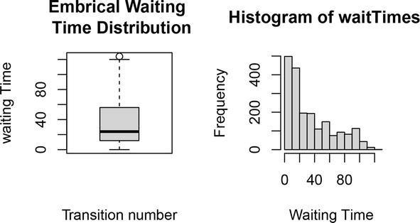
Figure 2.

Box plot and histogram of waiting times.

Detailed information that explores applications of HOMM and data sequence analysis using fuzzy sets are found in [15, 16, 17, 18]. Theory of Fuzzy sets was introduced by Zadeh [19].

3.3 Numerical evaluation of a simulated Ms/Ms/1/N queue

Now, with a simulation study of M = 1000 patients, we try to perform the queuing functions of a health care unit in a way that ensures the best results of an M_s/M_s/1/N queue. The processing time per customer is exponentially distributed with an average rate of μ = 0.27. Patients arrive randomly, with an average of one position every 4 minutes, and are treated on a first come, first served basis. The simulation route is run with an exponential arrival rate λ = 0.25 and an exponential service μ using r-code to implement the algorithm described above.

The r^th raw moment of the EQL is given by $\mathrm{E}\left({\mathrm{Y}}^r\right)={\mathrm{\Sigma }}_{j=0}^{N}j{\pi }_j.$

The estimated values of the all 2000 (= 1000 arrival point and 1000 departure epochs) transition epochs t_n: n = 1,2, …, 2000 and the corresponding waiting time W_n = L_n/λ of patients are calculated.

A box-and-whisker diagram of the waiting time distribution W_n: n = 1,2, …, 2000 and its histogram are displayed side by side in Figure 2. As expected, the box-and-whisker plot shows the sizes, spread, and skew of the interquartiles (Q1 = 12, Q2 = 24, Q3 = 56), max = 124, and whiskers (bottom = 0, top = 122) outside the upper and lower quartiles of waiting times. In addition, one exterior remains above the upper whisker, i.e., max W_n: n = 1,2, …, 2000 = 124. Using these facts together with some facts revealed by the histogram, we can conclude that the waiting time distribution can follow, approximately, an exponential distribution with a long tail to the right. A control chart (Figure 3) is designed to show additional information of the pair sequence {(t_n, W_n): n = 1,2,…,2000}.

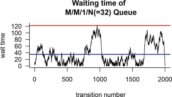
Figure 3.

Transition epochs vs. waiting times.

Any “health” management can refer to the Figure 3 and make certain decisions. First, management must maintain all types of resources necessary to treat and accommodate up to N = 32 patients, such as beds, medical equipment. Second, management can inform patients that the average waiting time is about 35 minutes and the maximum waiting time is about 124 minutes. If the administration installs an additional server during the transition periods of 995 and 1005, the patient’s waiting time can also be reduced. So this section explores how simulation technology can be used to build Markov-type queuing models and use it to better serve ordinary people.

4. Higher-order Markov model (HOMM)

This section discusses different characteristics of an higher-order Markov model (HOMM). The purpose is to explore briefly how a HOMM can be used in forecasting of time series observed over agricultural productions, stock market prices, oil demand, etc. The first step is to covert the given time series into a categorical sequence by fuzzifying the given time series {X(t): t = 0, 1, …,} over a finite number states $\in \mathbb{M}=\left\{1,2,\dots ,\mathrm{m}\right\}$. This type of forming of Markov categorical sequence was developed [20, 21].

The main advantage of using fuzzy logic is that it can handle imprecise data by assigning degrees of truth, called membership values in the closed interval [0,1]. It is an extension of the crisp method to a multivariate format. Since 1965, fuzzy set theory [19] has occupied various fields of our society, see [17, 18, 22]. For fitting a higher order multivariate Markov chain model, basic details can be found in Ref. [23].

We now focus on the data sequence {X_t = j}. Let the initial probability vectors of size “m” in canonical form be denoted by X_t = Pr(X_t = j) = (0, 0, …, 1, 0,…, 0)^T} for t = 0,1,…, n. Each m-vector X_t produces a conditional probability distribution of the categorical sequence for a given t. The corresponding normal form of the probability vector be $\overline{X}\left(t\right)=\frac{1}{n+1}{\sum }_{t=0}^n{\mathbf{X}}_t$.

Hence, each probability vector of size “m” of the sequence $\left\{\overline{X}\left(\mathrm{t}\right)=\left({\mathrm{x}}_1\left(\mathrm{t}\right),{\mathrm{x}}_2\left(\mathrm{t}\right),\dots ,{\mathrm{x}}_m\left(\mathrm{t}\right)\right)\right\}$ produces a conditional probability distribution of the categorical sequence for a given t. If the probability distribution at time t = r + 1 is dependent on the state probability vectors of t = r, r-1, r-2, .., r-n + 1, then the n^th order model is formulated as follows:

$${\overline{\mathbf{X}}}_{\mathrm{r}+1}=\sum _{\mathrm{h}=1}^{\mathrm{n}}{\lambda }_{\mathrm{h}}{\mathbf{P}}_{\mathrm{h}}{\overline{\mathbf{X}}}_{\mathrm{r}-\mathrm{h}+1}$$E30

The initial probability vectors are $\overline{X}\left(t\right):\mathrm{t}=0,1,\mathrm{..},\left(\mathrm{n}-1\right).{\lambda }_h$ are non-negative real numbers with ${\sum }_{h=1}^n{\lambda }_h=1$ and each P_h is the h-step transition probability matrix with each column sum equals unity for h = 1, 2, …, n. Numerical evaluation of P_h matrices and the scalars λ_h for h = 1, 2, …, n can be done with the “markovchain” package. Now, we can make use of the higher-order Markov model fitted by (19) for prediction future states after n-steps. The prediction of the next state $\overline{X}\left(\mathrm{t}\right)={\mathrm{P}}_{\left(t-1\right)}\overline{X}\left(\mathrm{t}‐1\right)$ at time t can be taken as the state with the maximum probability, i.e.,

$$\overline{X}\left(t\right)=j\text{if}\overline{X}\left(t\right)=k\le \overline{X}\left(t\right)=j\mathrm{k},\mathrm{j}=1,2,\dots \mathrm{m}$$E31

To evaluate the performance and effectiveness of the HOMM, a prediction error (PE) is defined (21):

$$\mathit{PE}=\frac{1}{K}\sum _{j=1}^K{\delta }_j\text{here}{\delta }_j=\left\{\begin{array}{c}1\text{if}{\overline{x}}_t=j\ne x_t\\ 0\text{if}{\overline{x}}_t=j=x_t\end{array}\right.$$E32

Example: Categorical data sequence and Fuzzy time series We now consider a hypothetical data on amount of rainfall (RF) time series X(t) = {x_t} observed from t = 1991 to t = 2001 years which is reported in Table 1. Let the universe of discourse of the ARF factor be U = [100, 1300]. We partition the set U into 4 equal length intervals as follows: u₁ = [100, 400), u₂ = [400, 700), u₃ = [700, 1000), u₄ = [1000, 1300] which are mutually disjoint such that $\mathrm{U}={\cup }_{\left(j=1\right)}^4{u}_j$.

Year	o(ARF)	o(S1)	E(S1)	E(ARF)	o(S2)	E(ARF)
1991	500.8	A2	NA	NA	NA	NA
1992	254.7	A1	A1	250	NA	NA
1993	982.3	A3	A3	850	A2A3	A2 A2
1994	590.9	A2	A2	550	A1A2	A1 A2
1995	153.4	A1	A1	250	A3A1	A3 A4
1996	875.4	A3	A3	850	A2A3	A2 A4
1997	1250.5	A4	A4	1150	A1A4	A1 A4
1998	1125.7	A4	A4	1150	A3A4	A3 A4
1999	622.6	A2	A2	550	A4A2	A4A2
2000	272	A1	A1	250	A4A1	A4A1
2001	623.4	A2	A3	850	A2A2	A2 A2

Table 1.

HOMM model fitting.

A Rainfall during 1991–2001. ARF = Rainfall amount, S1 = Linguistic Variable for ARF and expected states E(S1) from fitted Markov Model X_(t + 1) = P₁ X_t and X_(t) = P₂ X_(t − 1).

Let us define fuzzy sets to represent each division u_j of U through a linguistic variable, say A, as follows: A₁—low if x(t) ∈ u₁, A₂—medium if x(t) ∈ u₂, A₃—high if x(t) ∈ u₃, A₄—very high if x(t) ∈ u₄. Thus, there is a one to one correspondence between the rainfall amount x(t) received at time “t” and the values A_j for j = 1,2,3 and 4 of the linguistic variable A.

The observed categorical data sequence for the rainfall amount recorded in Table 1 is coded by S₁ = “2,” “1,” “3,” “2,” “1,” “3,” “4,” “4,” “2,” “1,” “2” or by S₁ = “A₂,” “A₁,” “A₃,” “A₂,” “A₁,” “A₃,” “A₄,” “A₄,” “A₂,” “A₁,” “A₂.” This representation given in the sequence S1 forms a fuzzy time series. In addition, the collection of all members of S₁ i.e., $\mathbb{S}=\left\{{}^{“}{{\mathrm{A}}_1}^{”},{}^{“}\mathrm{A}{2}^{”},{}^{“}\mathrm{A}{3}^{”},{}^{“}\mathrm{A}{4}^{”}\right\}$ can be viewed as the finite state space of a Markov Chain (MC) process over a period of time “t” but appropriate order of the MC is not known.

Using the sequence S₁, one can fit the first-order MC (FOMC) $\overline{X}\left(\mathrm{t}+1\right)={\lambda }_1\mathbf{P}\left(\mathrm{t}\right)\overline{X}\left(\mathrm{t}\right)$ for predicting the next state from a given state of the state space $\mathbb{S}=\left\{{}^{“}{{\mathrm{A}}_1}^{”},{}^{“}{{\mathrm{A}}_2}^{”},{}^{“}{{\mathrm{A}}_3}^{”},{}^{“}{{\mathrm{A}}_4}^{”}\right\}$.

By combining two adjacent states of the sequence S₁ of 11 elements, we can obtain the initial sequence S₂ = {A₂ A₁, A₁A₃, A₃A₂, A₂A₁, A₁A₃, A₃A₄, A₄A₄, A₄A₂, A₂A₁, A₁A₂} of 10 elements for constructing the second-order MC (SOMC). However, in each pair, say A_jA_k, the second position A_k is representing the current state since the Markov property forgets the past once the current state is known.

Fitting of First- and Second-order Markov models Let us fit FOMC to the observed sequence S₁ = “2,” “1,” “3,” “2,” “1,” “3,” “4,” “4,” “2,” “1,” “2” using the “markovchain’ software package applied in R-programming. The command fitHigherOrder(S₁,order = 2) is executed and the following results for the parameters of the HOMM given in (19) are obtained:

$${\overline{\mathbf{X}}}_{\mathrm{r}+1}={\lambda }_1{\mathbf{P}}_1{\overline{\mathbf{X}}}_{\mathrm{r}},\text{and},{\overline{\mathbf{X}}}_{\mathrm{r}+1}={\lambda }_1{\mathbf{P}}_1{\overline{\mathbf{X}}}_{\mathrm{r}}+{\lambda }_2{\mathbf{P}}_2{\overline{\mathbf{X}}}_{\left(\mathrm{r}-1\right)},r\ge 1$$E33

$${\overline{\mathbf{X}}}_0=\left(3/11,4/11,2/11,2/11\right),{\overline{\mathbf{X}}}_1=\left(3/10,2/10,3/10,2/10\right)$$

λ₁ = 0.5360825 and λ₂ = 0.4639175 = 1-λ₁.

Estimates of the transition matrices:

$${\widehat{P}}_1=\left(\begin{array}{llll}0& 1& 0& 0\\ 0.33& 0& 0.5& 0.5\\ 0.67& 0& 0& 0\\ 0& 0& 0.5& 0.5\end{array}\right){\widehat{P}}_2=\left(\begin{array}{llll}0& 0& 0.5& 0.5\\ 0.5& 0.33& 0.5& 0.5\\ 0& 0.67& 0& 0\\ 0.5& 0& 0.5& 0\end{array}\right)$$

Expected States to be reached in a single step:

Consider the fit ${\overline{\mathbf{X}}}_1={\lambda }_1{\mathbf{P}}_1{\overline{\mathbf{X}}}_0$. Because the first column of the matrix ${\widehat{P}}_1$ has the highest probability of 0.67 in the relation of the third row, which is the expected state after one step of state A.₁ is A₃, that is, A₁ → A₃. Thus, the expected AMR is calculated as the average of the limits from u₃ = [700, 1000), i.e., E(AMR) = (700 + 1000)/2 = 850.

The maximum probability of the second column of the matrix ${\widehat{P}}_1$ occurs in relation to the first row, starting from the observed state A₂, to which the MC would reach the state A₁ and the expected AMR, which is calculated from u₁ = [100 00) is 250. Our conclusion is A₂ → A₁.

The maximum probability (i.e., 0.5) of the third column of the matrix ${\widehat{P}}_1$ occurs in the second and fourth rows. Thus, starting from the considered state A₃, the MC would reach either state A₂ or A₄ and the expected AMR calculated by u₂ = [00700) is 550 and the expected AMR calculated by u₄ = [1000,1300) is 1150: P(A₃ → A₂) = P(A₃ → A₄) = 0.5.

The maximum probability of the fourth column of the matrix ${\widehat{P}}_1$ is 0.5 relative to rows 2 and 4. Thus, starting from the observed state A₄, the MC would reach either state A₂ or A₄, and the expected AMR calculated by u₂ = [400700) is 550 and the expected AMR calculated by u₄ = [1000,1300) is 1150: P(A₄ → A₂) = P(A₄ → A₄) = 0.5.

When comparing the states specified in columns o(ARF) and E(S₁) of the table-(\ref.*{T1}), the prediction error, or PE, is calculated using the formula (\ref) *{ER}): PE = (1/ 10) = 0.1.

Steady state stationary distribution $\overline{\mathbf{X}}$: Since the unit step transition probability matrix of the first order MC is ${\widehat{P}}_1$, the steady state stationary distribution $\overline{\mathbf{X}}$ is the solution of

$$\overline{\mathbf{X}}={\mathbf{P}}_1\overline{\mathbf{X}}$$E34

Executing the command steadyStates(P₁) in the “markovchain” package in R code, we obtain that $\overline{\mathbf{X}}=\left(0.3,0.3,0.2,0.2\right)$.

Second-order MC: Steady state stationary distribution ${\overline{\mathbf{X}}}^{\left(\mathbf{2}\right)}$ Consider the initial sequence S₂ = {A₂ A₁, A₁A₃, A₃A₂, A₂A₁, A₁A₃, A₃A₄, A₄A₄, A₄A₂, A₂A₁, A₁A₂} of 10 elements for constructing the SOMC. Each state has a pair of items such as A_jA_k in which A_k is the current state. We now discuss the analysis of the model fit using the estimates of λ values and the TPMs in the following expression:

$${\overline{\mathbf{X}}}_2={\lambda }_1{\mathbf{P}}_1{\mathbf{X}}_1+{\lambda }_2{\mathbf{P}}_2{\overline{\mathbf{X}}}_0$$E35

Applying the similar arguments on the factor ${\overline{\mathbf{X}}}_1={\mathbf{P}}_2{\overline{\mathbf{X}}}_0$, we can arrive at the following conclusions: C1: A₁ → A₂ or A₁ → A₄.

$${\mathrm{A}}_2\to {\mathrm{A}}_3$$

$${\mathrm{A}}_3\to {\mathrm{A}}_1\text{or}{\mathrm{A}}_3\to {\mathrm{A}}_4$$

$${\mathrm{A}}_4\to {\mathrm{A}}_1\text{or}{\mathrm{A}}_2\to {\mathrm{A}}_2$$

Repeating the similar exercise on the factor ${\overline{\mathbf{X}}}_2={\mathbf{P}}_1{\overline{\mathbf{X}}}_1$, we can arrive at the following conclusions:

$$\text{C2}$$

$${\mathrm{A}}_1\to {\mathrm{A}}_3$$

$${\mathrm{A}}_2\to {\mathrm{A}}_1$$

$${\mathrm{A}}_3\to {\mathrm{A}}_2\text{or}{\mathrm{A}}_3\to {\mathrm{A}}_4$$

$${\mathrm{A}}_4\to {\mathrm{A}}_2\text{or}{\mathrm{A}}_4\to {\mathrm{A}}_4$$

Now, ordering the results of C1 with C2 in this order we obtain the expected second-order sequences at the end of the second state: A₁ A₁ or A₁ A₂ or A₁ A₄.

$${\mathrm{A}}_2{\mathrm{A}}_2\text{or}{\mathrm{A}}_2{\mathrm{A}}_4$$

$${\mathrm{A}}_3{\mathrm{A}}_3\text{or}{\mathrm{A}}_3{\mathrm{A}}_2,{\mathrm{A}}_3{\mathrm{A}}_4$$

$${\mathrm{A}}_4{\mathrm{A}}_1\text{or}{\mathrm{A}}_4{\mathrm{A}}_2\text{or}{\mathrm{A}}_4{\mathrm{A}}_4$$

All these results are reported in Table 1.

Prediction error for SOMC fit is PE = (3/9) = 0.33.

It can be shown that the matrix P = λ₁P₁ + λ₂P₂ serves as the TPM of the SOMC. Hence, the steady state stationary distribution ${\overline{\mathbf{X}}}^{\left(\mathbf{2}\right)}$ can be obtained by solving the equation ${\overline{\mathbf{X}}}^{\left(\mathbf{2}\right)}\mathbf{P}={\overline{\mathbf{X}}}^{\left(\mathbf{2}\right)}.{\overline{\mathbf{X}}}^{\left(\mathbf{2}\right)}=\left(0.2673632,0.3203355,0.1946253,0.2176760\right)$.

The prediction error of the FOMC is smaller than that of second-order MC. In addition, there is no significant improvement in the four component stationary probability vector ${\overline{\mathbf{X}}}^{\left(\mathbf{2}\right)}$ as compared to the respective components of first-order vector $\overline{\mathbf{X}}$. So we can conclude that the fFOMC is preferable over the SOMC for future predictions.

5. Conclusion

This chapter looked at three types of Markov models. The first model addressed the basic issues of a warehouse connected to an M/M/1/N/FCFS facility. The long-run probability distributions of queue length and inventory variables were obtained using matrix methods. The expected total cost function was formulated based on holding costs, ordering costs, and waiting time cost and was used to obtain the optimal order quantity. A graphical representation of the relationship between the cost function and order quantity was provided to support the theoretical results of this model.

The second model investigated the changes made by the arrival and departure phases of the M/M/1/N/FCFS queue and thus analyzed the simulated queue M_s/M_s/1/N for long-term evaluation of moments. The input queue length and waiting times for all consecutive transitions in the M_s/M_s/1/N system were calculated and all were plotted on a control chart to observe the effect of the customer waiting time distribution.

The third model analyzed the HOMM to predict the fuzzy time series as a data series. Two special cases, the FOMC and the SOMC, were fitted to the same dataset generated by measuring the hypothetical rainfall ensemble. Forecast errors for both FOMC and SOMC were calculated and compared to show that the FOMC performed best.

The best conclusions are thus made by analyzing MC models for both waiting line and inventory problems. We developed either numerically tractable expressions or accurate probabilistic expressions to obtain numerical representations. The first model can be recommended for any QIM problem and the second model to quickly assess waiting times in medical resources to ensure the best quality of service. A third model can be conveniently used to predict future states of categorical datasets with higher orders.

Future research will develop intelligent and easy-to-implement algorithms for the interdisciplinary researchers.

Conflict of interest

The author declares no conflict of interest.

Thanks declaration

The author would like to thank two colleagues for their comments on Markov models, which greatly helped this chapter of the book.

References

1.Gross D, Harris SM. Fundamentals of Queueing Theory. 3rd ed. New York, NY: Wiley; 1998
2.Bhat N. An Introduction to Queueing Theory: Modeling and Analysis in Applications. 2nd ed. Boston: Birkhauser; 2008. p. 268. DOI: 10.1007/978-0-8176-4725-4
3.Spedicato GA. Discrete Time Markov Chains with R. The R Journal. 2017. Available from: https://journal.r-project.org/archive/2017/RJ-2017-036/index.html
4.Hunter JJ. Filtering of Markov renewal queues, II: Birth-death queues. Advanced in Application Problem. 1983;15:376-391
5.Sivasamy R, Jayanthi S. Charts for detecting small shifts. Economic Quality Control. 2003;8(1):1-8
6.Sivasamy R, Thillaigovindan N, Paulraj G, Paranjothi N. Quasi-birth and death processes of two server queues with stalling. OPSEARCH. 2019;56:739-756. DOI: 10.1007/s12597-019-00376-1
7.Sivasamy R. An M/M(1)+M(2)/1 queue with a state dependent K-policy. Journal of Xi’an University of Architecture & Technology. 2021;I:111-124
8.Taylor HM, Karlin S. An Introduction to Stochastic Modeling. 3rd edition. San Deigo, CA: Academic Press; 1998. ISBN-10: 0126848874, ISBN-13: 978-0126848878
9.Zhang Y, Yue D, Sun L, Zuo J. Analysis of the queueing-inventory systems with impatient customers and mixed sales. Discrete Dynamics in Nature and Soceity. 2022;2022:1-12. DOI: 10.1155/2022/2333965
10.Alnowibet KA, Alrasheedi AF, Alqahtani FS. Queueing models for analysing the steady-state distribution of stochastic inventory systems with random Lead time and impatient customers. Process. 2022;10:1-24. DOI: 10.3990//pr10040624
11.Daduna H, Szekli R. M/M/1 queueing systems with inventory. Queueing System. 2006;54:55-78. DOI: 10.1007/s11134-006-8710-5
12.Schwarz M, Daduna H. Queueing systems with inventory management with random lead times and with backordering. Mathematical Methods of Operational Research. 2006;64:383-414
13.Latouche G, Ramaswami V. Introduction to Matrix Analytic Methods in Stochastic Modeling: ASA-SIAM Series on Statistics and Applied Probability. Philadelphia, PA: SIAM; 1999
14.Shore H. General control charts for attributes. IIE Transactions. 2000;32(12):1149-1160
15.Berman O, Kim E. Stochastic models for inventory management at service facilities. Communication Statistical Stochastic Model. 1999;15(4):695-718
16.Berman O, Kim E. Dynamic order replenishment policy in internet-based supply chains. Mathematical Method Operations Research. 2001;2001:53
17.Song Q, Chissom BS. Forecasting enrollments with fuzzy time series – Part I. Fuzzy Sets and Systems. 1993;54:1-9
18.Wong W-K, Bai E, Chu AW. Adaptive time-variant models for fuzzy-time-series forecasting. IEEE Transaction System on Man Cybernetics: Part B. 2010;40:1531-1542
19.Zadeh LA. Fuzzy sets. Information and Control. 1965;8(3):338-353. DOI: 10.1016/S0019-9958(65)90241-X
20.Ching WK, Fung ES, Ng MK. Higher-Order Markov Chain models for categorical data sequences. Naval Research Logistics. 2004;2004:557-574. DOI: 10.1002/nav.20017
21.Ching WK, Ng MK, Fung ES. Higher-order multivariate Markov chains and their applications. Linear Algebra and Its Applications. 2008;428:492-506
22.Singh P, Borah B. Forecasting stock index price based on M-factors fuzzy time series and particle swarm optimization. International Journal of Approximate Reasoning. 2014;55:812-833. DOI: 10.1016/j.ijar.2013.09.014
23.Sivasamy R, Senthamaraikannan K, Adebayo Fatai A, Karuppasamy KM. Higher order Markov chain fitting for data on rainfall and Rice production. YMER. 2021;20(10):156-170
Written By
Sivasamy Ramasamy and Wilford B. Molefe
Submitted: 18 December 2022Reviewed: 09 March 2023Published: 26 April 2023
Open access peer-reviewed chapter