Existence of Limit Cycles for a Class of Quintic Kukles Homogeneous System

Abstract

We investigated the existence of limit cycles for quintic Kukles polynomial differential systems depending on a parameter in this chapter. These systems are important in practical applications and theoretical advances. We first used formal series method based on Poincaré’s ideas to prove this point and determine the center-focus problem. We then utilized the Dulac function to prove the nonexistence of closed orbits. We determined the sufficient condition for the existence of the limit cycles, which bifurcate from the equilibrium point, using Hopf bifurcation theory. Lastly, we provided some numerical examples for illustration using MATLAB to plot. Note that studies on the existence and the nonexistence of limit cycles and algebraic limit cycles for Kukles systems are limited.

1. Introduction

Limit cycle discovery by Poincaré in his paper Integral Curves defined by differential equations (1881–1886) [1, 2, 3, 4]. Physicists [5] failed to describe the oscillation phenomenon through the linear differential equation in the twentieth century. Van der Pol [6] proposed van der Pol equation in 1926 to describe the oscillation of the constant amplitude of a triode vacuum tube.

The limit cycle has attracted the attention of many pure and applied mathematicians. Numerous mathematical models from physics, biology, economics, engineering, and chemistry have been proposed since the 1950s to explore autonomous plane systems with a limit cycle [5, 7]. Limit cycle theory is closely related to Hilbert’s 16th problem. Exploring the existence of limit cycles is crucial in this theory. Poincaré proposed the method of topographical system, the successor function, small parameter method, and the annular region theorem to determine the existence of limit cycles. Existence, nonexistence, uniqueness, and other properties of the limit cycle have been extensively analyzed by mathematicians and physicists [8].

The problem of the existence of periodic solutions in the Liénard equation was explored in a previous study [9].

$$\ddot{x}+f\left(x\right)\dot{x}+g\left(x\right)=0.$$E1

This problem has been widely investigated since the study of Liénard. The Liénard equation in the phase plane is equivalent to the system

$$\begin{array}{c}\frac{\mathit{dx}}{\mathit{dt}}=y,\\ \frac{\mathit{dy}}{\mathit{dt}}=-g\left(x\right)-f\left(x\right)y.\end{array}$$E2

The Liénard equation in the Liénard plane is equivalent to the system and can be expressed as follows:

$$\begin{array}{c}\frac{\mathit{dx}}{\mathit{dt}}=y-F\left(x\right),\\ \frac{\mathit{dy}}{\mathit{dt}}=-g\left(x\right),\end{array}$$E3

where $F\left(x\right)={\int }_0^{x}f\left(x\right)\mathit{dx}$. On this basis, the problem of the existence of periodic solutions is brought back to a problem of the existence of limit cycles for the previous systems (3).

For the more general equation

$$\ddot{x}+f\left(x,\dot{x}\right)\dot{x}+g\left(x\right)=0.$$E4

We observed that the Liénard system (3) has become invalid because $f$ depends on two variables. Meanwhile, the phase plane system (2) can be transformed into the following formula:

$$\begin{array}{c}\frac{\mathit{dx}}{\mathit{dt}}=y,\\ \frac{\mathit{dy}}{\mathit{dt}}=-g\left(x\right)-f\left(x,y\right)y.\end{array}$$E5

Accordingly, several limit cycles exist [9]. The problem of limit cycles of the Eq. (4) was first explored by Norman Levinson, Oliver K. Smith, and Dragilev [5].

Our work is related to the differential system of the following form:

$$\frac{\mathit{dx}}{\mathit{dt}}=y,$$

$$\frac{\mathit{dy}}{\mathit{dt}}=-x+P_n\left(x,y\right),$$E6

where $P_n\left(x,y\right)$ is a homogeneous polynomial of the degree $n$. System (6) contains a center point at the origin if and only if this system is symmetric to one of the coordinate axes because $n\ge 2.$ The Russian mathematician I. S. Kukles first investigated differential polynomial systems (6) in 1944. System (6) was then called the Kukles homogeneous systems [10, 11, 12]. The polynomial differential system (6) is linear when $n=1.$ Obtaining isolated periodic solutions in the set of all periodic solution linear differential systems is impossible. The polynomial differential system (6) is a quadratic system when $n=2$, in which the system is symmetric to the $y$-axis; and this system has been extensively investigated [13]. The cubic system (6) was examined when n = 3 to obtain a system (6) that has six small amplitude limit cycles in the neighborhood of the origin [6, 14, 15]. Rebiha Benterki and Jaume Llibre examined system (6), which is symmetric to the $y-\mathit{\text{axis}}$, when n = 4 in 2017 and provides a sufficient condition for the existence of limit cycles [10]. The system (6) always contains either a center or a fine focus (weak focus) at the origin.

Consider the polynomial differential system

$$\frac{\mathit{dx}}{\mathit{dt}}=-y,$$

$$\frac{\mathit{dy}}{\mathit{dt}}=x+b_1{x}^2+b_2\mathit{xy}+b_3{y}^2+b_4{x}^3+b_5{x}^{2}y+b_{6}x{y}^2+b_7{y}^3.$$E7

Kukles provided the necessary and sufficient conditions for the origin to be centered. However, some new cases have been discovered. C. J. Christopher and N. G. Lloyd [16] explored the case $b_7=0$, (reduced Kukles system) in 1990 and established the system (7), which contains a maximum of five limit cycles bifurcating from the origin. N. G. Lloyd [17] and J. M. Pearson [18] analyzed the case $b_2=0$ in 1990 and established system (7), which contains a maximum six limit cycles bifurcating from the origin. The central problem is to characterize between a center and a focus at the origin of the system. If all orbits in the neighborhood spiral toward or away from the origin, then the origin is the focus. If all orbits in the neighborhood, except the origin, are periodic, then the origin is the center. This problem of characterizing between a center and a focus at the origin has been solved only in linear and quadratic systems. However, a few particular cases in families of high degree still require further investigation. Some studies have discussed the existence and the nonexistence of small amplitude limit cycles and algebraic limit cycles for Kukles systems. A previous study proved that system (7) with nonlinearities of a degree higher than two contains a center at the origin if and only if its vector field is symmetric to one of the coordinate axes in 2015 [11].

We present some necessary definitions and theorems in the first section of this chapter. We used a formal series method based on Poincaré’s ideas to determine the center focus in the second section. By the Hopf bifurcation theory, we obtained the sufficient condition for existence of limit cycles for a following quintic Kukles polynomial differential system depending on a parameter

$$\frac{\mathit{dx}}{\mathit{dt}}=y,$$

$$\frac{\mathit{dy}}{\mathit{dt}}=-x-2x^3+b_{21}{x}^{2}y+b_{12}x{y}^2+b_{50}{x}^5+b_{41}{x}^{4}y,$$E8

where $b_{21},b_{12},b_{50}$ and $b_{41}$ are parameters, and $x$ and $y$ are real variables that bifurcate from the equilibrium point (singular point). Hence, we establish sufficient conditions for the existence of the limit cycle according to the change analysis of the stability of the focus when the parameters change. Lastly, we presented some numerical examples for illustration. Notably, system (8) contains several limit cycles and the Liénard system is used to prove that the existence is already invalid.

2. Some preliminary results

In this section, we introduce some definitions and notations regarding the existence of the quintic differential system (8).

2.1 Conjecture

The origin, except for the linear center, is not the isochronous center of system (7) if the system has odd degree. Therefore, if the linear term contains a center, and the degree of the nonlinear term is odd, then the origin cannot be the center simultaneously.

2.2 Local results for Liénard systems

Blows and Lloyd proved the following results for system (2) in 1989, where $f\left(x\right)=a_0+a_{1}x+a_2{x}^2+\dots +a_m{x}^m$and $g\left(x\right)=x+b_2{x}^2+b_3{x}^3+\dots +b_n{x}^n$, $m$ and $n$are the natural numbers. Let $H\left(m,n\right)$ denote the maximum numbers of small-amplitude limit cycles that can be bifurcated from the origin for system (2), where $m$ is the degree of $f$ and $n$ is the degree of $g$. If $g$is odd and the order of $f=m=2i\mathit{\text{or}}2i+1$, then $H\left(m,n\right)=i$ [19].

3. Singular point for system

The singular points for system (8) are $\mathit{A}\left(\mathbf{0},\mathbf{0}\right)$, $\mathit{B}\left(\sqrt[\mathbf{2}]{\left(\frac{\mathbf{1}\mathbf{+}\sqrt{\mathbf{1}\mathbf{+}{\mathit{b}}_{\mathbf{50}}}}{{\mathit{b}}_{\mathbf{50}}}\right)},\mathbf{0}\right)$,$\mathit{C}\left(\mathbf{-}\sqrt[\mathbf{2}]{\left(\frac{\mathbf{1}\mathbf{+}\sqrt{\mathbf{1}\mathbf{+}{\mathit{b}}_{\mathbf{50}}}}{{\mathit{b}}_{\mathbf{50}}}\right)},\mathbf{0}\right)$, $\mathit{D}\left(\sqrt[\mathbf{2}]{\left(\frac{\mathbf{1}\mathbf{-}\sqrt{\mathbf{1}\mathbf{+}{\mathit{b}}_{\mathbf{50}}}}{{\mathit{b}}_{\mathbf{50}}}\right)},\mathbf{0}\right)$ and $\mathit{E}\left(\mathbf{-}\sqrt[\mathbf{2}]{\left(\frac{\mathbf{1}\mathbf{-}\sqrt{\mathbf{1}\mathbf{+}{\mathit{b}}_{\mathbf{50}}}}{{\mathit{b}}_{\mathbf{50}}}\right)},\mathbf{0}\right)\mathbf{.}$

Remark 1

1. The following cases are presented for singular points $B\mathit{\text{and}}C:$

   1. If $b_{50}=-1,$ then points $\mathit{\text{B}}\mathit{\text{and}}C$ $\in \mathbb{C}$, and $\mathbb{C}$ is a complex number.

   2. If $b_{50}<-1$, then points $B\mathit{\text{and}}C\in \mathbb{C}$.

   3. If $-1<b_{50}<0$, then the points $B\mathit{\text{and}}C\in \mathbb{C}$.

   4. If $b_{50}>0,$ then points $B\mathit{\text{and}}C\in ℝ$(real number).

2. The following cases are presented for singular points $D\mathit{\text{and}}E:$

   1. If $b_{50}=-1,$then points $\mathit{\text{D}}\mathit{\text{and}}E$ $\in \mathbb{C}$.

   2. If $b_{50}>1,$ then points $D\mathit{\text{and}}E\in \mathbb{C}$.

   3. If $b_{50}<-1$, then points $D\mathit{\text{and}}E\in \mathbb{C}.$

   4. If $0<b_{50}<1,$ then points $D\mathit{\text{and}}E\in \mathbb{C}$.

   5. If $-1<b_{50}<0,$ then points $D\mathit{\text{and}}E\in \mathbb{C}.$

Note: Singular points $D\mathit{\text{and}}E$ are not investigated in this study because we consider $x\mathit{\text{and}}y$ as real variables.

Note: The linear system contains the center [20]. However, the perturbation of these centers inside the class of the linear differential system fails to produce a limit cycle because a linear differential system cannot contain an isolated periodic solution in the set of all periodic solutions.

4. Nonlinear system

For system (8) the associated nonlinear system gave by calculating the following Jacobian matrix:

$$J\left(x,y\right)=\left(\begin{array}{cc}0& 1\\ -1-6x^2+2b_{21}\mathit{xy}+b_{12}{y}^2+5b_{50}{x}^4+4b_{41}{x}^{3}y& b_{21}{x}^2+2b_{12}\mathit{xy}+b_{41}{x}^4\end{array}\right)$$

The characteristic equation is

$$={\lambda }^2-\left(b_{21}{x}^2+2b_{12}\mathit{xy}+b_{41}{x}^4\right)\lambda -\left(-1-6x^2+2b_{21}\mathit{xy}+b_{12}{y}^2+5b_{50}{x}^4+4b_{41}{x}^{3}y\right)=0$$

Let $\mathit{Tr}=-\left(b_{21}{x}^2+2b_{12}\mathit{xy}+b_{41}{x}^4\right)$,

$$\mathit{det}=-\left(-1-6x^2+2b_{21}\mathit{xy}+b_{12}{y}^2+5b_{50}{x}^4+4b_{41}{x}^{3}y\right),$$

then the characteristic equation is $D\left(\lambda \right)={\lambda }^2+\mathit{Tr\lambda }+\mathit{det}=0$.

Its roots are

$${\lambda }_1,{\lambda }_2=\frac{-\mathit{Tr}\mp \sqrt{{\mathit{Tr}}^2-4\mathit{det}}}{2}$$

1. For singular point $\mathit{B}\left(\sqrt[\mathbf{2}]{\left(\frac{\mathbf{1}\mathit{+}\sqrt{\mathbf{1}\mathit{+}{\mathit{b}}_{\mathbf{50}}}}{{\mathit{b}}_{\mathbf{50}}}\right)},\mathbf{0}\right)$ of system (8) and $b_{50}>0$, the Jacobian matrix

   $$J\left(\sqrt[\mathbf{2}]{\left(\frac{\mathbf{1}\mathit{+}\sqrt{\mathbf{1}\mathit{+}{\mathit{b}}_{\mathbf{50}}}}{{\mathit{b}}_{\mathbf{50}}}\right)},\mathbf{0}\right)=\left(\begin{array}{cc}0& 1\\ -1-6x_0^2+5b_{50}{x}_0^4& b_{21}{x}_0^2+b_{41}{x}_0^4\end{array}\right)$$

   where $x_0=\sqrt[\mathbf{2}]{\left(\frac{\mathbf{1}+\sqrt{\mathbf{1}+{\mathit{b}}_{\mathbf{50}}}}{{\mathit{b}}_{\mathbf{50}}}\right)}$

   The characteristic equation is

   $${\lambda }^2-\left(b_{21}{x}_0^2+b_{41}{x}_0^4\right)\lambda -\left(-1-6x_0^2+5b_{50}{x}_0^4\right)=0$$

   Its roots are

   $${\lambda }_{1,2}=\frac{\left(b_{21}{x}_0^2+b_{41}{x}_0^4\right)\pm \sqrt{{\left(b_{21}{x}_0^2+b_{41}{x}_0^4\right)}^2+4\left(-1-6x_0^2+5b_{50}{x}_0^4\right)}}{2}$$

   $\left(-1-6x_0^2+5b_{50}{x}_0^4\right)$ can be written as $5b_{50}{y}^2-6y-1=0$. Then

   $$y_{1,2}=\frac{6\pm \sqrt{36+20b_{50}}}{10b_{50}}$$

   When $36+20b_{50}>0$ and $b_{50}>0$, then the two roots ${\lambda }_{1,2}$ are real roots with different signs. Then the singular point $\mathit{B}\left(\sqrt[\mathbf{2}]{\left(\frac{\mathbf{1}\mathit{+}\sqrt{\mathbf{1}\mathit{+}{\mathit{b}}_{\mathbf{50}}}}{{\mathit{b}}_{\mathbf{50}}}\right)},\mathbf{0}\right)$ is a saddle.

2. For singular point $\mathit{C}\left(\mathit{-}\sqrt[\mathbf{2}]{\left(\frac{\mathbf{1}\mathit{+}\sqrt{\mathbf{1}\mathit{+}{\mathit{b}}_{\mathbf{50}}}}{{\mathit{b}}_{\mathbf{50}}}\right)},\mathbf{0}\right)$ of system (8) when and $b_{50}\ne 0,$ the Jacobian matrix

   $$J\left(\mathit{-}\sqrt[\mathbf{2}]{\left(\frac{\mathbf{1}\mathit{+}\sqrt{\mathbf{1}\mathit{+}{\mathit{b}}_{\mathbf{50}}}}{{\mathit{b}}_{\mathbf{50}}}\right)},\mathbf{0}\right)=\left(\begin{array}{cc}0& 1\\ -1-6x_0^2+5b_{50}{x}_0^4& b_{21}{x}_0^2+b_{41}{x}_0^4\end{array}\right)$$

   The characteristic equation is

   $${\lambda }^2-\left(b_{21}{x}_0^2+b_{41}{x}_0^4\right)\lambda -\left(-1-6x_0^2+5b_{50}{x}_0^4\right)=0$$

   where $x_0=-\sqrt[\mathbf{2}]{\left(\frac{\mathbf{1}+\sqrt{\mathbf{1}+{\mathit{b}}_{\mathbf{50}}}}{{\mathit{b}}_{\mathbf{50}}}\right)}$

   Its roots are

   $${\lambda }_{1,2}=\frac{\left(b_{21}{x}_0^2+b_{41}{x}_0^4\right)\pm \sqrt{{\left(b_{21}{x}_0^2+b_{41}{x}_0^4\right)}^2+4\left(-1-6x_0^2+5b_{50}{x}_0^4\right)}}{2}$$

   $\left(-1-6x_0^2+5b_{50}{x}_0^4\right)$ can be rewritten as $5b_{50}{y}^2-6y-1=0$, then

   $$y_{1,2}=\frac{6\pm \sqrt{36+20b_{50}}}{10b_{50}}$$

   When $36+20b_{50}>0$ and $b_{50}>0$, then the two roots ${\lambda }_{1,2}$ are real roots with different signs. Then the singular point $\mathit{C}\left(\mathit{-}\sqrt[\mathbf{2}]{\left(\frac{\mathbf{1}\mathit{+}\sqrt{\mathbf{1}\mathit{+}{\mathit{b}}_{\mathbf{50}}}}{{\mathit{b}}_{\mathbf{50}}}\right)},\mathbf{0}\right)$, is a saddle.

3. The Jacobian matrix for the singular point $A\left(0,0\right)$ of system (8) is $J\left(0,0\right)=\left(\begin{array}{cc}0& 1\\ -1& 0\end{array}\right)$

Its characteristic equation is λ² + 1 = 0 ⇒ λ = ±i ; then the singular point for the nonlinear system (8) is difficult to distinguish whether the singular point $A\left(0,0\right)$ is a center or a focus, so we will use the formal series method to decide it. We will show the detailed process in the next section.

5. Center-focus

Determining the center focus in the qualitative theory of differential equations, especially for the plane of the high-order polynomial differential system, is difficult and troublesome. According to the Hopf bifurcation theory, when we analyze the conditions of the limit cycle branching from the equilibrium point and the stability of the generated cycle, we must make a detailed analysis of the central focus. The qualitative analysis of a class of high-order differential systems is presented in this chapter. It is obvious that $A\left(0,0\right)$ is the center of the linear system corresponding to the system (8). We need to determine the center focus problem of singularity $A\left(0,0\right)$ of the nonlinear system. We use the formal series method based on Poincaré’s ideas to examine the behavior of singularity $A\left(0,0\right)$.

6. Main results

6.1 Determination of the center-focus

Theorem 1 The following are assumed for system (8):

1. If $b_{21}>0,$then the point $A\left(0,0\right)$is the first-order unstable weak focus.

2. If $b_{21}<0,$ then the point $A\left(0,0\right)$ is the first-order stable weak focus.

3. If $b_{21}=0,b_{41}>0,$ then the point $A\left(0,0\right)$ is the second-order unstable weak focus.

4. If $b_{21}=0,b_{41}<0,$ then the point $A\left(0,0\right)$ is the second-order stable weak focus

5. If $b_{21}=0,b_{41}=0,$ then the point $A\left(0,0\right)$ is the center.

Proof Suppose the system (8) has a solution of the following series form, then

$$F\left(x,y\right)=x^2+y^2+\sum _{k=3}^{\infty }{F}_k\left(x,y\right),$$

where $F_k$ is the $k$-degree homogeneous polynomial of $x$ and $y$. Then,

$${\left.\frac{\mathit{dF}}{\mathit{dt}}\right|}_{\left(8\right)}=\frac{\partial F}{\partial x}\frac{\mathit{dx}}{\mathit{dt}}+\frac{\partial F}{\partial y}\frac{\mathit{dy}}{\mathit{dt}}$$

$$=\left(2x+\sum _{k=3}^{\infty }\frac{\partial F_x}{\partial x}\right)\left(y\right)$$

$$+\left(2y+\sum _{k=3}^{\infty }\frac{\partial F_x}{\partial y}\right)(-x-2x^3+b_{21}{x}^{2}y$$

$$+b_{12}x{y}^2+b_{50}{x}^5+b_{41}{x}^{4}y)$$E9

At the right end of the above equation, starting from the third term, by making the homogeneous equations of the same order equal to zero, we can obtain series equations as follows:

Let the third power term at the right end of the Formula (9) be zero. We obtain

$$x\frac{\partial F_3}{\partial y}-y\frac{\partial F_3}{\partial x}=2\left(x{P}_2+y{Q}_2\right)=0$$

We take the polar coordinate of the above formula $x=rcos\theta ,y=rsin\theta ,r^2=x^2+y^2$ and remove $r^3$.

$$\frac{d{F}_3\left(cos\theta ,sin\theta \right)}{\mathit{d\theta }}=0,$$

$$F_3\left(cos\theta ,sin\theta \right)=\mathit{\text{constant}},$$

$$F_3\left(x,y\right)=\mathit{\text{constant}}.$$

Let the term of power four at the right end of the formula (9) be zero, we find

$$x\frac{\partial F_4}{\partial y}-y\frac{\partial F_4}{\partial x}=2\left(x{P}_3+y{Q}_3\right)+\left(P_2\frac{\partial F_3}{\partial x}+Q_2\frac{\partial F_3}{\partial y}\right)$$

$$=-4x^{3}y+2b_{21}{x}^2{y}^2+2b_{12}{\mathit{xy}}^3.$$

Similarly, we use polar coordinates to find$F_4$ and remove$r^4$ to obtain

$$D_4=\frac{d{F}_4\left(cos\theta ,sin\theta \right)}{\mathit{d\theta }}=-4{\mathit{cos}}^3\theta sin\theta +2b_{21}{\mathit{cos}}^2\theta {\mathit{sin}}^2\theta$$

$$+2b_{12}cos\theta {\mathit{sin}}^3\theta .$$

We discuss three situations as follows:

First case: ${\mathit{b}}_{\mathbf{21}}\mathbf{\ne }\mathbf{0}\mathbf{.}$

Since

$${\int }_0^{2\pi }-4{\mathit{cos}}^3\theta sin\theta +2b_{21}{\mathit{cos}}^2\theta {\mathit{sin}}^2\theta +2b_{12}cos\theta {\mathit{sin}}^3\mathit{\theta d\theta }\ne 0.$$

We take $F_4$ to satisfy the equation

$$\frac{d{F}_4\left(cos\theta ,sin\theta \right)}{\mathit{d\theta }}=D_4-C_4,$$

where

$$C_4=\frac{b_{21}}{\pi }{\int }_0^{2\pi }{\mathit{cos}}^2\theta {\mathit{sin}}^2\mathit{\theta d\theta }.$$

$C_4$ has the same sign as$b_{21}$ . Thus, $C_4=\frac{b_{21}}{4}$ . If

$$V\left(x,y\right)=x^2+y^2+F_3+F_4.$$

Then,

$${\left.\frac{\mathit{dV}}{\mathit{dt}}\right|}_{\left(8\right)}=C_4{r}^4+O\left(r^4\right).$$

When$b_{21}>0,\mathit{\text{the point}}A\left(0,0\right)$ is the first-order unstable weak focus.

When$b_{21}<0,\mathit{\text{the point}}A\left(0,0\right)$ is the first-order stable weak focus.

Second case: $b_{21}=0,b_{41}\ne 0$. Thus,

$$\frac{d{F}_4\left(cos\theta ,sin\theta \right)}{\mathit{d\theta }}=-4{\mathit{cos}}^3\theta sin\theta +2b_{12}cos\theta {\mathit{sin}}^3\theta ,$$

$$F_4\left(cos\theta ,sin\theta \right)={\mathit{cos}}^4\theta +\frac{b_{12}{\mathit{sin}}^4\theta }{2},$$

$$F_4\left(x,y\right)=x^4+\frac{b_{12}}{2}{y}^4.$$

Simplify (note that $b_{21}=0$)

Let the term of power five at the end of the formula (9) be zero, then

$$x\frac{\partial F_5}{\partial y}-y\frac{\partial F_5}{\partial x}=2\left(x{P}_4+y{Q}_4\right)+\sum _{k=3}^4\left(P_{5-k+1}\frac{\partial F_k}{\partial x}+Q_{5-k+1}\frac{\partial F_k}{\partial y}\right),$$

$$=2\left(x{P}_4+y{Q}_4\right)+\left(P_3\frac{\partial F_3}{\partial x}+Q_3\frac{\partial F_3}{\partial y}\right)+\left(P_2\frac{\partial F_4}{\partial x}+Q_2\frac{\partial F_4}{\partial y}\right),$$

$$=\left(-2x^3+b_{21}{x}^{2}y+b_{12}x{y}^2\right)\frac{\partial F_3}{\partial y}.$$

Given that $F_3=\mathit{\text{constant}},$then $\frac{\partial F_3}{\partial y}=0$. Thus,

$$x\frac{\partial F_5}{\partial y}-y\frac{\partial F_5}{\partial x}=0.$$

We take the polar coordinate of the above and remove $r^5$ to obtain

$$\frac{d{F}_5\left(cos\theta ,sin\theta \right)}{\mathit{d\theta }}=0,$$

$$F_5\left(cos\theta ,sin\theta \right)=\mathit{\text{constant}},$$

$$F_5\left(x,y\right)=\mathit{\text{constant}}.$$

Simplify (note that $b_{21}=0$)

Let the term of power six at the end of the formula (9) be zero, then

$$x\frac{\partial F_6}{\partial y}-y\frac{\partial F_6}{\partial x}=2\left(x{P}_5+y{Q}_5\right)+\sum _{k=3}^5\left(P_{6-k+1}\frac{\partial F_k}{\partial x}+Q_{6-k+1}\frac{\partial F_k}{\partial y}\right),$$

$$=2\left(x{P}_5+y{Q}_5\right)+\left(P_4\frac{\partial F_3}{\partial x}+Q_4\frac{\partial F_3}{\partial y}\right),$$

$$+\left(P_3\frac{\partial F_4}{\partial x}+Q_3\frac{\partial F_4}{\partial y}\right)+\left(P_2\frac{\partial F_5}{\partial x}+Q_2\frac{\partial F_5}{\partial y}\right),$$

$$=2b_{50}{x}^{5}y+2b_{41}{x}^4{y}^2+\left(-2x^3+b_{12}x{y}^2\right)\frac{\partial F_4}{\partial y}.$$

When $b_{21}=0$, $F_4\left(x,y\right)=x^4+\frac{b_{12}}{2}{y}^4$, $\frac{\partial F_4}{\partial y}=2b_{12}{y}^3$ .Thus,

$$x\frac{\partial F_6}{\partial y}-y\frac{\partial F_6}{\partial x}=2b_{50}{x}^{5}y+2b_{41}{x}^4{y}^2-4b_{12}{x}^3{y}^3+2b_{12}^{2}x{y}^5.$$

We take the polar coordinate of the above equation and remove $r^6$to obtain

$$D_6=\frac{d{F}_6\left(cos\theta ,sin\theta \right)}{\mathit{d\theta }}=2b_{50}{\mathit{cos}}^5\theta sin\theta +2b_{41}{\mathit{cos}}^4\theta {\mathit{sin}}^2\theta$$

$$-4b_{12}{\mathit{cos}}^3\theta {\mathit{sin}}^3\theta +2b_{12}^{2}cos\theta {\mathit{sin}}^5\theta .$$

When $b_{41}\ne 0$,

$${\int }_0^{2\pi }2b_{50}{\mathit{cos}}^5\theta sin\theta +2b_{41}{\mathit{cos}}^4\theta {\mathit{sin}}^2\theta -4b_{12}{\mathit{cos}}^3\theta {\mathit{sin}}^3\theta +2b_{12}^{2}cos\theta {\mathit{sin}}^5\mathit{\theta d\theta }\ne 0.$$

We take $F_6$ to satisfy the equation as follows:

$$\frac{d{F}_6\left(cos\theta ,sin\theta \right)}{\mathit{d\theta }}=D_6-C_6,$$

where $C_6=\frac{b_{41}}{\pi }{\int }_0^{2\pi }{\mathit{cos}}^4\theta {\mathit{sin}}^2\mathit{\theta d\theta }$,$C_6=\frac{b_{41}}{8}.$

$C_6$has the same sign as $b_{41}$. If

$$V\left(x,y\right)=x^2+y^2+F_3+F_4+F_5+F_6,$$

$${\left.\frac{\mathit{dV}}{\mathit{dt}}\right|}_{\left(8\right)}=C_6{r}^6+O\left(r^6\right).$$

When$b_{21}=0,b_{41}>0,\mathit{\text{the point}}A\left(0,0\right)$ is the second-order unstable weak focus.

When $b_{21}=0,b_{41}<0,\mathit{\text{the point}}A\left(0,0\right)$ is the second-order stable weak focus.

Third case: $b_{21}=0,b_{41}=0.$

Given that $P\left(-x,y\right)=P\left(x,y\right)$and $Q\left(-x,y\right)=-Q\left(x,y\right),$the vector field ($P\left(x,y\right),Q\left(x,y\right))$is symmetrical with respect to the y-axis. Hence, point $A\left(0,0\right)$ is the center.

6.2 Nonexistence of limit cycle

Theorem 2 If one of the following conditions is satisfied, then closed orbits are absent in the whole plane of system (8).

1. $b_{12}<0,b_{21}>0,b_{41}\ge 0;$

2. $b_{12}<0,b_{21}\ge 0,b_{41}>0;$

3. $b_{12}\le 0,b_{21}>0,b_{41}>0;$

4. $b_{12}>1,b_{21}\le 0,b_{41}<0;$

5. $b_{12}>1,b_{21}<0,b_{41}\le 0;$

6. $b_{12}\ge 1,b_{21}<0,b_{41}<0.$

Proof When $b_{12}\ne 0,b_{50}=0$, let

$$L\left(y\right)=b_{12}y-1$$

$${\left.\frac{\mathit{dL}\left(y\right)}{\mathit{dt}}\right|}_{\left(8\right)}=b_{12}\dot{y}$$

$$=\left(1-b_{12}\right)x+b_{21}{x}^2-2b_{12}{x}^3+b_{41}{x}^4$$

Thus, $y=\frac{1}{b_{12}}$ is the line and not the tangent of the trajectory of the system (8). The Dulac’s function is $B=\frac{1}{b_{12}y-1}$ (when $b_{12}\ne 0$). Then,

$${\left.\mathit{div}\left(\mathit{BP},\mathit{BQ}\right)\right|}_{\left(8\right)}=-\frac{\left(1-b_{12}\right)x+b_{21}{x}^2-2b_{12}{x}^3+b_{41}{x}^4}{{\left(b_{12}y-1\right)}^2}$$

We obtain ${\left.\mathit{div}\left(\mathit{BP},\mathit{BQ}\right)\right|}_{\left(8\right)}\le 0$ when the condition (1), (2), or (3) holds.

We obtain ${\left.\mathit{div}\left(\mathit{BP},\mathit{BQ}\right)\right|}_{\left(8\right)}\ge 0$ when the condition (4), (5), or (6) holds.

When any one of the conditions in Theorem 2 is satisfied, then ${\left.\mathit{sgn}\mathit{div}\left(\mathit{BP},\mathit{BQ}\right)\right|}_{\left(8\right)}$ is definite. Moreover, ${\left.\mathit{div}\left(\mathit{BP},\mathit{BQ}\right)\right|}_{\left(8\right)}=0,$ if and only if, $x=0$. In other words, it is not identically zero in any subregion in the $\left(x,y\right)$ plane. Thus, the system (8) has no closed orbits in the whole plane under any one of the cases in this theorem.

Theorem 3 When $b_{21}=0,b_{41}=0,$ then the system (8) has no limit cycle.

Proof Since $\mathit{div}\left(\mathit{PB},\mathit{QB}\right)\mathit{\equiv }\mathbf{0}$, so the system (8) has a continuous differentiable integral factor $B\left(x,y\right)$, there is no limit cycle. The simulation is presented in Figure 1.

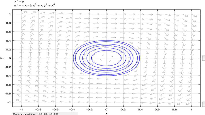
Figure 1.

Center for nonlinear system.

6.3 Existence of limit cycles

Theorem 4 The system (8) contains at least one limit cycle around A(0,0) when one of the following conditions is true:

1. $b_{21}>0,$

2. $b_{21}<0,$

3. $b_{21}=0,b_{41}>0,$

4. $b_{21}=0,b_{41}<0.$

Proof The singular point $A\left(0,0\right)$ is an unstable and weak focus point of system (8) under the conditions (1) and (3). Singularity $A\left(0,0\right)$ of the system (8) changes from an unstable weak focus to a stable focus. According to Hopf bifurcation theory, the system (8) generates at least one unstable limit cycle around the point $A\left(0,0\right)$ under the changes in these parameters.

Under the conditions (2) and (4), singular point $A\left(0,0\right)$ is the stable and weak focus point of the system (8). The singularity $A\left(0,0\right)$ of the system (8) changes from stable, weak focus to an unstable focus. According to Hopf bifurcation theory, under the changes in these parameters, the system (8) generates at least one stable limit cycle around $A\left(0,0\right)$ (point)

Theorem 5 System (8) contains at least two small-amplitude limit cycles bifurcating from the origin $A\left(0,0\right).$

Proof If Theorem 4 holds, then there are perturbations of system (8) yielding two small-amplitude limit cycles bifurcating from the origin. According to Theorem 1, we determine that system (8) has two weak focus points. We denote the number of weak focus as $k$, and $k=2$. The system (8) is a class quintic; thus, we denote n as $n=5.$ We determine that the system (8) has two limit cycles around the $A\left(0,0\right).$

Theorem 6 System (8) contains a maximum of two limit cycles when $b_{12}=0$.

Proof When $b_{12}=0,$ the system (8) transforms to the following form:

$$\frac{\mathit{dx}}{\mathit{dt}}=y,$$

$$\frac{\mathit{dy}}{\mathit{dt}}=-x-2x^3+b_{21}{x}^{2}y+b_{50}{x}^5+b_{41}{x}^{4}y.$$

This system is equivalent to the following system:

$$\begin{array}{c}\frac{\mathit{dx}}{\mathit{dt}}=y,\\ \frac{\mathit{dy}}{\mathit{dt}}=-g\left(x\right)-f\left(x\right)y,\end{array}$$

where $g\left(x\right)=-x-2x^3+b_{50}{x}^5$ and $f\left(x\right)=b_{21}{x}^2+b_{41}{x}^4$. $g\left(x\right)$is odd, and the degree of $f\left(x\right)=4$is even based on the definition of the local result of the Liénard system and the results of Blows and Lloyd. The maximum number of small-amplitude limit cycles bifurcated from the origin is two.

6.4 Numerical solution

Example 1 If we set the following parameters in system (8):$b_{21}=1,b_{12}=1,b_{41}=1$, and $b_{50}=1,$ then a limit cycle exists around $A\left(0,0\right)$. The simulation is presented in Figure 2.

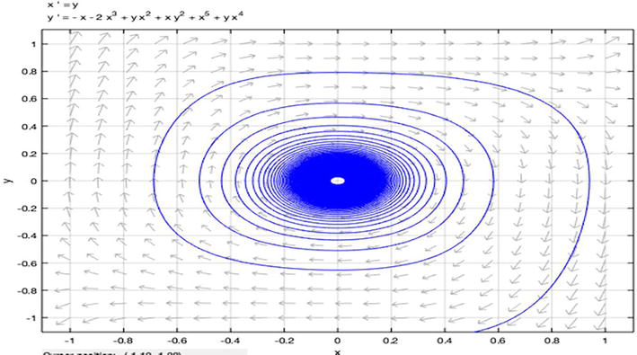
Figure 2.

Existence of the limit cycle for system (8), when${\mathrm{b}}_{21}=1,{\mathrm{b}}_{12}=1,{\mathrm{b}}_{41}=1,$ and ${\mathrm{b}}_{50}=1.$

Example 2 If we set the following parameters in the system (8):$b_{12}=1,b_{21}=-1,b_{41}=1,$ and $b_{50}=1$, then a limit cycle exists around $A\left(0,0\right)$ according to Theorem 4 of the existence of limit cycle (Case 2). There exists a limit cycle around. The simulation is presented in Figure 3.

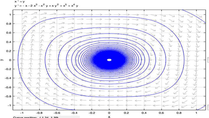
Figure 3.

Existence of the limit cycle for system (8), when ${\mathrm{b}}_{12}=1,{\mathrm{b}}_{21}=-1,{\mathrm{b}}_{41}=1,$and ${\mathrm{b}}_{50}=1$.

If we set the following parameters in the system (8): $b_{12}=1,b_{21}=0.5,b_{41}=1,$ and $b_{50}=1$, then a limit cycle exists around $A\left(0,0\right)$ according to Theorem 4 of the existence of limit cycle (Case 1). The simulation is presented in Figure 4.

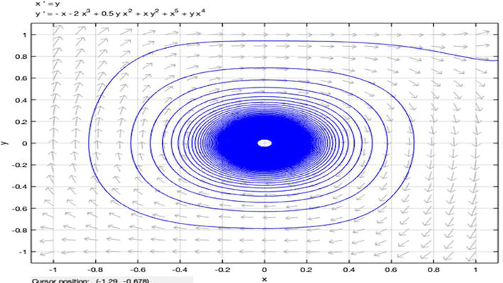
Figure 4.

Existence of the limit cycle for system (8), when ${\mathrm{b}}_{12}=1,{\mathrm{b}}_{21}=0.5,{\mathrm{b}}_{41}=1,$ and ${\mathrm{b}}_{50}=1$.

If we set the following parameters in the system (8): $b_{12}=1,b_{21}=0,b_{41}=1,$ and $b_{50}=1$, then a limit cycle exists around $A\left(0,0\right)$ according to Theorem 4 of the existence of limit cycle (Case 3). The simulation is presented in Figure 5.

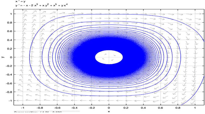
Figure 5.

Existence of the limit cycle for system (8), when ${\mathrm{b}}_{12}=1,{\mathrm{b}}_{21}=0,{\mathrm{b}}_{41}=1,$and ${\mathrm{b}}_{50}=1$.

If we set the following parameters in the system (8): $b_{12}=1,b_{21}=0,b_{41}=-0.5,$ and $b_{50}=1$, then a limit cycle exists around $A\left(0,0\right)$ according to Theorem 4 of the existence of limit cycle (Case 4). The simulation is presented in Figure 6.

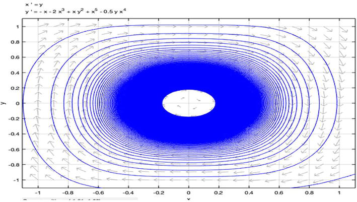
Figure 6.

Existence of the limit cycle for system (8), when ${\mathrm{b}}_{12}=1,{\mathrm{b}}_{21}=0,{\mathrm{b}}_{41}=-0.5$, and ${\mathrm{b}}_{50}=1.$

7. Conclusions

We investigated the existence of the limit cycle and used the formal series method to determine the center-focus in this chapter.

We establish the sufficient conditions for the existence of the limit cycles in system (8) that bifurcate from the equilibrium point using Hopf bifurcation theory and discuss the nonexistence of closed orbits using the Dulac function. Some examples were provided for illustration.

A number of interesting problems arise from this work. Future research in this area could include finding a general solution formula that can be used for algebraic equations of higher degrees and the calculation of system singularity. Such problems offer researchers a wealth of opportunities to expand this new area.

Acknowledgments

The authors are grateful to both reviewers for their helpful suggestions and comments.

Conflict of interest

The authors declare no conflict of interest.

Thanks

The authors are grateful to Prof. Ivana Barac for her help and cooperation.

References

- 1.
Poincaré H. Mémoire sur les courbes définies par une équation différentielle (II). Journal of Maths and Pures Applications. 1882; 8 :251-296. Available from:http://eudml.org/doc/235914 - 2.
Poincaré H. Mémoire sur les courbes définies par une équation différentielle (I). Journal of Maths and Pures Applications. 1881; 7 (I):375-422 - 3.
Poincaré H. Sur les courbes définies par les équations différentielles (III). Journal of Maths and Pures Applications. 1885; 1 (4):167-244 - 4.
Poincaré H. Sur les courbes definies par les equations differentielles(IV). Euvres de Henri Poincaré. 1985; 1 (Iv):85-162 - 5.
Ye Y-Q et al. Theory of limit cycles. The American Mathematical Society. 1986; 66 - 6.
Han M, Lin Y, Yu P. A study on the existence of limit cycles of a planar system with third-degree polynomials. International Journal of Bifurcation and Chaos. 2004; 14 (1):41-60. DOI: 10.1142/S0218127404009247 - 7.
Mattuck A. LC. Limit Cycles. Journal of Differential Equations. 2011; 2011 :1-6 - 8.
Cao J. Limit cycles of polynomial differential systems with homogeneous nonlinearities of degree 4 via the averaging method. Journal of Computational and Applied Mathematics. 2008; 220 (1–2):624-631. DOI: 10.1016/j.cam.2007.09.007 - 9.
Cioni M, Villari G. An extension of Dragilev’s theorem for the existence of periodic solutions of the Liénard equation. Nonlinear Analysis: Theory, Methods & Applications. 2015; 127 :55-70. DOI: 10.1016/j.na.2015.06.026 - 10.
Benterki R, Llibre J. Centers and limit cycles of polynomial differential systems of degree 4 via averaging theory. Journal of Computational and Applied Mathematics. 2017; 313 :273-283. DOI: 10.1016/j.cam.2016.08.047 - 11.
Giné J, Llibre J, Valls C. Centers for the Kukles homogeneous systems with odd degree. The Bulletin of the London Mathematical Society. 2015; 47 (2):315-324. DOI: 10.1112/blms/bdv005 - 12.
Giné J, Llibre J, Valls C. Centers for the kukles homogeneous systems with even degree. Journal of Applied Analytical Computers. 2017; 7 (4):1534-1548. DOI: 10.11948/2017093 - 13.
Bautin N. On the number of limit cycles appearing with variation of the coefficients from an equilibrium state of the type of a focus or a center. Maths Science Net. 1952; 1 (1939):2414 - 14.
Lloyd NG, Pearson JM. Computing centre conditions for certain cubic systems. Journal of Computational and Applied Mathematics. 1992; 40 (3):323-336. DOI: 10.1016/0377-0427(92)90188-4 - 15.
Hong Z, et al. Limit cycles for the Kukles system. Journal of Dynamical and Control Systems. 2008; 14 (2):283-298. DOI 10.1007/s10883-008-9036-x - 16.
Christopher CJ, Lloyd NG. On the paper of jin and wang concerning the conditions for a Centre in certain cubic systems. The Bulletin of the London Mathematical Society. 1990; 22 (1):5-12. DOI: 10.1112/blms/22.1.5 - 17.
Chow SN, Li C, Wang D. Normal Forms and Bifurcation of Planar Vector Fields. Cambridge University Press. 1994 - 18.
Munoz R. Introduction to Bifurcations and the Hopf Bifurcation Theorem for Planar Systems. Colarado State University; 2011. pp. 11-14 - 19.
Lynch S. Dynamical Systems with Applications Using MapleTM. Springer Science & Business Media; 2009 - 20.
Zhang Zhi-fen HW. Qualitative Theory of Differential Equations. United States of America: American Mathematical Society; 1991