Generalized Quantum Polynomials

Abstract

On a general time scale, polynomials, Taylor’s formula, and related subjects are described in terms of implicit and inefficient recursive relations. In this work, our primary goal is to construct proper polynomials, namely delta and nabla generalized quantum polynomials, on (q, h)-time scales explicitly. We show that generalized quantum polynomials play the same roles on (q, h)-time scales as ordinary polynomials play in $\mathbb{R}$ since they obey the additive properties and Leibnitz rules. Such polynomials which recover falling/rising and q-falling/q-rising factorials are constructed by the frame of forward and backward shifts. Additionally, we present delta- and nabla-Gauss’ binomial formulas which provide many applications.

1. Introduction

The polynomials occupy a very significant place in the theory of analysis. Once a polynomial is constructed, it is possible to express not only elementary functions but also some special functions in terms of infinite series of polynomials. On the other hand, a contribution to polynomials provides progress also on the theory of differential/difference equations because they could be proposed or solved by the frame of polynomials. Since the creation of modern calculus, the polynomials have been studied on continuous line or on discrete lattice where the stepsize $h$ is constant, namely on $h\mathbb{Z}$

$$h\mathbb{Z}≔\left\{\mathit{hx}:x\in \mathbb{Z},h\in {\mathbb{R}}^{+}\right\},$$E1

or on quantum numbers where the stepsize is not uniform, namely on ${\mathbb{K}}_q$

$${\mathbb{K}}_q≔\left\{q^n:q\in \mathbb{R},q\ne 1,n\in \mathbb{Z}\right\}\cup \left\{0\right\}.$$E2

After the invention of time scales by Stefan Hilger [1], many mathematical concepts constructed on discrete sets and continuous sets are unified without any big obstacles, especially in the theory of difference/differential equations. However, some key mathematical concepts such as polynomials and Taylor’s formula have inefficient or implicit recursive definitions on general time scales and they are inapplicable in practice. Therefore, these concepts are studied not on a general time scale but instead on some specific time scales such as on (1) or on (2).

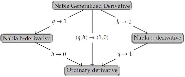
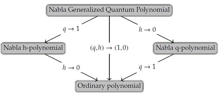
The so-called $\left(q,h\right)$-time scale ${\mathbb{T}}_{\left(q,h\right)}$ is introduced by Čermák and Nechvátal [2] as the unification of (1) and (2) in order to study fractional calculus. The importance of the $\left(q,h\right)$-time scale is beyond the expectations. In this special setting, it is possible to study the mathematical concepts which cannot be presented explicitly on a general time scale. In this work, we aim to present the proper forms of the polynomials on ${\mathbb{T}}_{\left(q,h\right)}$ in a manner that they assure the nature of $\left(q,h\right)$-time scales. In the literature, the studies on time scales proceed in two directions due to the delta and nabla derivative operators. For that reason, we present the unified polynomials on ${\mathbb{T}}_{\left(q,h\right)}$ in two separate forms: delta and nabla generalized quantum polynomials. We analyze the fundamental properties of both generalized quantum polynomials. One of the most significant advantage of studying on ${\mathbb{T}}_{\left(q,h\right)}$ is to attain the results which reduce to the results on $h\mathbb{Z}$, $\mathbb{K}q$ and $\mathbb{R}$ in the proper limits of $h$ and $q$. We emphasize that the nabla generalized quantum polynomial unifies

1. nabla $q$-polynomial as $h\to 0$,

2. nabla $h$-polynomial as $q\to 1$,

3. ordinary polynomial as $\left(q,h\right)\to \left(1,0\right)$,

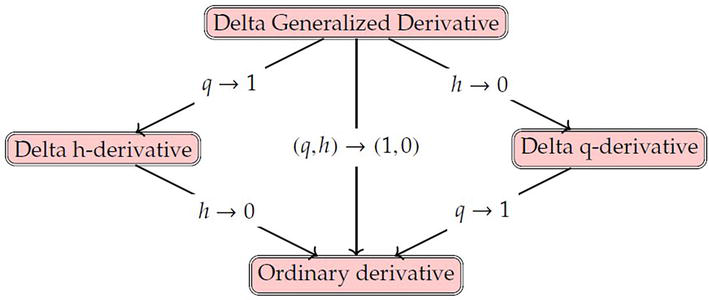
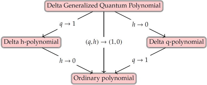
while the delta generalized quantum polynomial recovers

1. delta $q$-polynomial as $h\to 0$,

2. delta $h$-polynomial as $q\to 1$,

3. ordinary polynomial as $\left(q,h\right)\to \left(1,0\right)$.

The details of the above reductions under proper limits will be analyzed throughout the current work. Since the construction of ${\mathbb{T}}_{\left(q,h\right)}$ is well-defined, the reductions of forward and backward shifts, the nabla and delta derivatives, polynomials, Gauss Binomial formula to $h\mathbb{Z}$, ${\mathbb{K}}_q$ and $\mathbb{R}$ are consistent in both nabla and delta sense.

The current work is organized as follows. In Section 2, we give a very brief introduction to time scale calculus, define two appropriate $\left(q,h\right)$-time scales and we state the concepts of $\left(q,h\right)$-time scale calculus (in both nabla and delta sense). Section 3 is devoted to present the nabla generalized quantum polynomial equipped with its key features such as derivative rule and additive property. We also state and prove the nabla $\left(q,h\right)$-Taylor’s formula from which we are able to establish the nabla $\left(q,h\right)$-Gauss binomial formula. In Section 4, we intensify on the delta generalized quantum polynomial. It is shown that the delta version of quantum binomial also possesses the key features of the polynomials. The delta version of $\left(q,h\right)$-Taylor’s formula and Gauss binomial formula is presented. The notions and theories are explained by examples.

2. Preliminaries

A time scale $\mathbb{T}$ is a non-empty closed subset of $\mathbb{R}$. The most well-known examples of time scales: $\mathbb{Z}$, the Cantor set $\mathcal{C}$ and the discrete sets $h\mathbb{Z}$ (1) and ${\mathbb{K}}_q$ (2). We refer readers to see the pioneering article [1] and the books [3, 4] for the details of the theory of time scales and [5, 6, 7] for $\left(q,h\right)$-calculus. In this section, we only list the concepts of calculus on time scales, nabla calculus on ${\mathbb{T}}_{\left(q,h\right)}^1$ and delta calculus on ${\mathbb{T}}_{\left(q,h\right)}^2$ which we require throughout this work.

On an arbitrary time scale $\mathbb{T}$, the forward jump and the backward jump operators are given by

$$\sigma \left(x\right)≔inf\left\{s\in \mathbb{T}:s>x\right\},\rho \left(x\right)≔sup\left\{s\in \mathbb{T}:s<x\right\}.$$E3

The $\mathrm{\Delta }$- and $\nabla$-derivatives of a real-valued function on $\mathbb{T}$, are, respectively, defined by

$$f^{\mathrm{\Delta }}\left(x\right)≔\underset{s\to x}{lim}\frac{f\left(\sigma \left(s\right)\right)-f\left(x\right)}{\sigma \left(s\right)-x},$$E4

$$f^{\nabla }\left(x\right)≔\underset{s\to x}{lim}\frac{f\left(\rho \left(s\right)\right)-f\left(x\right)}{\rho \left(s\right)-x}.$$E5

For given $h,q\in {\mathbb{R}}^{+}$, we introduce two-parameter time scales by

$${\mathbb{T}}_{\left(q,h\right)}^1≔\left\{q^{n}x+\left[n\right]h:n\in \mathbb{Z}\right\}\cup \left\{\frac{h}{1-q}\right\},q>1,x>\frac{h}{1-q},$$E6

or

$${\mathbb{T}}_{\left(q,h\right)}^2≔\left\{q^{n}x+\left[n\right]h:n\in \mathbb{Z}\right\}\cup \left\{\frac{h}{1-q}\right\},0<q<1,x<\frac{h}{1-q},$$E7

where $\left[n\right]$ stands for the $q$-number given by

$$\left[n\right]≔1+q+\cdots +q^{n-1},$$E8

which tends to the non-negative integer $n$ as $q\to 1$. It is clear that such time scales are generalizations of (1) and (2). On ${\mathbb{T}}_{\left(q,h\right)}^1$ and ${\mathbb{T}}_{\left(q,h\right)}^2$, the operators $\sigma$ and $\rho$ reduce to

$$\sigma \left(x\right)=\mathit{qx}+h,\rho \left(x\right)=\frac{x-h}{q}.$$E9

The point $\frac{h}{1-q}$ is an accumulation point, because of the limits

$$\underset{n\to \infty }{lim}\left(q^{n}x+\left[n\right]h\right)=\frac{h}{1-q},0<q<1$$E10

and

$$\underset{n\to \infty }{lim}{q}^{-n}\left(x-\left[n\right]h\right)=\frac{h}{1-q},q>1.$$E11

The reason why we separately define (6) and (7) is to make our contributions consistent with the general theory of time scales.

Remark 2.1. It is also possible to define ${\mathbb{T}}_{\left(q,h\right)}^1$ for $0<q<1,x<\frac{h}{1-q}$ and define ${\mathbb{T}}_{\left(q,h\right)}^2$ for $q>1,x>\frac{h}{1-q}$. However, in those cases, the roles of the operators $\sigma$ and $\rho$ have to interchange in order to be consistent with the definitions (3).

Here we note that the time scales ${\mathbb{T}}_{\left(q,h\right)}^1$ and ${\mathbb{T}}_{\left(q,h\right)}^2$ are purely discrete sets with the exceptional accumulation point $\frac{h}{1-q}$. The nabla $\left(q,h\right)$-derivative and the delta $\left(q,h\right)$-derivative are defined as follows.

Definition 2.2. [7] Let $f\left(x\right):{\mathbb{T}}_{\left(q,h\right)}^1\to \mathbb{R}$ be a function. The nabla $\left(q,h\right)$-derivative of $f$ is defined by

$${\stackrel{\sim }{D}}_{\left(q,h\right)}f\left(x\right)≔\left\{\begin{array}{ll}\frac{f\left(x\right)-f\left(\frac{x-h}{q}\right)}{x-\left(\frac{x-h}{q}\right)}& \text{if}x\ne \frac{h}{1-q},\\ \underset{s\to {\left(\frac{h}{1-q}\right)}^{+}}{lim}\frac{f\left(s\right)-f\left(\frac{h}{1-q}\right)}{s-\frac{h}{1-q}}& \text{if}x=\frac{h}{1-q},\end{array}\right.$$E12

provided that the limits exist (see [3], Theorem 1.16 i).

Definition 2.3. [2, 5] Let $f\left(x\right):{\mathbb{T}}_{\left(q,h\right)}^2\to \mathbb{R}$ be a function. The delta $\left(q,h\right)$-derivative of $f$ is defined by

$$D_{\left(q,h\right)}f\left(x\right)≔\left\{\begin{array}{ll}\frac{f\left(\mathit{qx}+h\right)-f\left(x\right)}{\mathit{qx}+h-x}& \text{if}x\ne \frac{h}{1-q},\\ \underset{s\to {\left(\frac{h}{1-q}\right)}^{-}}{lim}\frac{f\left(s\right)-f\left(\frac{h}{1-q}\right)}{s-\frac{h}{1-q}}& \text{if}x=\frac{h}{1-q},\end{array}\right.$$E13

provided that the limits exist (see [3], Theorem 1.16 i).

One of the most significant advantage of $\left(q,h\right)$ time scales is to allow us to study $q$-calculus, $h$-calculus, and ordinary calculus on one hand. By the definition of jump operators (9), these operators reduce to

1. $\sigma \left(x\right)={\sigma }_h\left(x\right)=x+h$ and $\rho \left(x\right)={\rho }_h\left(x\right)=x-h$ as $q\to 1$.

2. $\sigma \left(x\right)={\sigma }_q\left(x\right)=\mathit{qx}$ and $\rho \left(x\right)={\rho }_q\left(x\right)=\frac{x}{q}$ as $h\to 0$.

3. $\sigma \left(x\right)=\rho \left(x\right)=x$ as $\left(q,h\right)\to \left(1,0\right)$.

The above reductions have very interesting consequences. If the above reductions are applied to the nabla $\left(q,h\right)$-derivative (12), we obtain the following list of reductions.

1. $\mathbb{T}={\mathbb{K}}_q$: The nabla $q$-derivative ${\tilde{D}}_{\left(q,0\right)}f\left(x\right)={\nabla }_{q}f\left(x\right)$.

2. $\mathbb{T}=h\mathbb{Z}$: The nabla $h$-derivative ${\tilde{D}}_{\left(1,h\right)}f\left(x\right)={\nabla }_{h}f\left(x\right)$.

3. $\mathbb{T}=\mathbb{R}$: The ordinary derivative ${\tilde{D}}_{\left(1,0\right)}f\left(x\right)=\frac{\mathit{df}\left(x\right)}{\mathit{dx}}$.

Similarly, the delta $\left(q,h\right)$-derivative (13) has the below list of reductions.

1. $\mathbb{T}={\mathbb{K}}_q$: The delta $q$-derivative [8] $D_{\left(q,0\right)}f\left(x\right)={\mathrm{\Delta }}_{q}f\left(x\right)$.

2. $\mathbb{T}=h\mathbb{Z}$: The nabla $h$-derivative $D_{\left(1,h\right)}f\left(x\right)={\mathrm{\Delta }}_{h}f\left(x\right)$.

3. $\mathbb{T}=\mathbb{R}$: The ordinary derivative $D_{\left(1,0\right)}f\left(x\right)=\frac{\mathit{df}\left(x\right)}{\mathit{dx}}$.

The above reductions are shown in Figures 1 and 2.

Figure 1.

Reductions of the nabla generalized derivative (or nabla $\left(q,h\right)$-derivative).

Figure 2.

Reductions of the delta generalized derivative (or delta $\left(q,h\right)$-derivative).

Proposition 2.4. [7] If $f,g:{\mathbb{T}}_{\left(q,h\right)}^1\to \mathbb{R}$ are any functions then the product rule for nabla $\left(q,h\right)$-derivative is given by

$${\tilde{D}}_{\left(q,h\right)}\left(f\left(x\right)g\left(x\right)\right)=g\left(x\right){\tilde{D}}_{\left(q,h\right)}f\left(x\right)+f\left(\frac{x-h}{q}\right){\tilde{D}}_{\left(q,h\right)}g\left(x\right)$$E14

$$=f\left(x\right){\tilde{D}}_{\left(q,h\right)}g\left(x\right)+g\left(\frac{x-h}{q}\right){\tilde{D}}_{\left(q,h\right)}f\left(x\right).$$E15

Proposition 2.5. [5] If $f,g$ are any real-valued functions defined on ${\mathbb{T}}_{\left(q,h\right)}^2$, then the product rule for delta $\left(q,h\right)$-derivative is expressed as

$$D_{\left(q,h\right)}\left(f\left(x\right)g\left(x\right)\right)=g\left(x\right)D_{\left(q,h\right)}f\left(x\right)+f\left(\mathit{qx}+h\right)D_{\left(q,h\right)}g\left(x\right)$$E16

$$=f\left(x\right)D_{\left(q,h\right)}g\left(x\right)+g\left(\mathit{qx}+h\right)D_{\left(q,h\right)}f\left(x\right).$$E17

Definition 2.6. We introduce the $\frac{1}{q}$-number as

$${\left[m\right]}_{\frac{1}{q}}≔1+\frac{1}{q}+\frac{1}{q^2}+\cdots +\frac{1}{q^{m-1}},m\in \mathbb{N}.$$E18

Similar to the $q$-number $\left[m\right]$, the $\frac{1}{q}$-number approaches to the non-negative number $m$ as $q\to 1$. Moreover, there is a relation between $q$ and $\frac{1}{q}$-numbers

$${\left[m\right]}_{\frac{1}{q}}=\frac{{\left[m\right]}_q}{q^{m-1}}.$$E19

Definition 2.7. We introduce the $\frac{1}{q}$-factorial by

$${\left[m\right]}_{\frac{1}{q}}!={\left[m\right]}_{\frac{1}{q}}{\left[m-1\right]}_{\frac{1}{q}}\cdots {\left[1\right]}_{\frac{1}{q}},m\in \mathbb{N},$$E20

while ${\left[0\right]}_{\frac{1}{q}}!≔1$.

Definition 2.8. We introduce the $\frac{1}{q}$-binomial coefficient as

$${\left[\begin{array}{c}m\\ j\end{array}\right]}_{\frac{1}{q}}≔\frac{{\left[m\right]}_{\frac{1}{q}}!}{{\left[m-j\right]}_{\frac{1}{q}}!{\left[j\right]}_{\frac{1}{q}}!},0\le j\le m,m\in \mathbb{N}.$$E21

Proposition 2.9. The following properties hold for the $\frac{1}{q}$-binomial coefficient

$${\left[\begin{array}{c}m\\ i\end{array}\right]}_{\frac{1}{q}}={\left[\begin{array}{c}m\\ m-i\end{array}\right]}_{\frac{1}{q}},$$E22

$${\left[\begin{array}{c}m\\ i\end{array}\right]}_{\frac{1}{q}}=q^{i\left(i-m\right)}{\left[\begin{array}{c}m\\ i\end{array}\right]}_q.$$E23

Proof: By Definition 2.8, the property (i) is clear. For (ii), we employ the relation (19) which leads to

$${\left[\begin{array}{c}m\\ j\end{array}\right]}_{\frac{1}{q}}=\frac{{\left[m\right]}_{\frac{1}{q}}!}{{\left[m-i\right]}_{\frac{1}{q}}!{\left[i\right]}_{\frac{1}{q}}!}=q^{i\left(i-m\right)}\frac{{\left[m\right]}_q!}{{\left[m-j\right]}_q!{\left[j\right]}_q!}=q^{i\left(i-m\right)}{\left[\begin{array}{c}m\\ i\end{array}\right]}_q.$$E24

3. Nabla generalized quantum polynomial

In this Section, our main aim is to present nabla $\left(q,h\right)$-analog of the polynomial ${\left(x-\omega \right)}^m$ on ${\mathbb{T}}_{\left(q,h\right)}^1$ (6) in a way that such a polynomial is consistent with the nabla $\left(q,h\right)$-derivative operator (12) and preserves the properties similar to ordinary polynomials. The findings of this section are based on the work [7].

Definition 3.1. We define the nabla generalized quantum polynomial (or nabla $\left(q,h\right)$-polynomial) by

$${\left(x-\omega \right)}_{\widetilde{q,h}}^m≔\left\{\begin{array}{ll}1& \text{if}m=0,\\ \prod _{j=1}^m\left(x-\frac{\omega -\left[j-1\right]h}{q^{j-1}}\right)& \text{if}m\in \mathbb{N},\omega \in \mathbb{R}.\end{array}\right.$$E25

Example 3.2. We can demonstrate the nabla $\left(q,h\right)$-polynomial (25) for $m=4$

$${\left(x-\omega \right)}_{\widetilde{q,h}}^4=\left(x-\omega \right)\left(x-\frac{\omega -h}{q}\right)\left(x-\frac{\omega -\left[2\right]h}{q^2}\right)\left(x-\frac{\omega -\left[3\right]h}{q^3}\right).$$E26

1. If we set $h=\frac{1}{2}$ and $q=2$, then $\left[2\right]=1+q\to 3$ and $\left[3\right]=1+q+q^2\to 7$ and (26) turns out to be

   $${\left(x-\omega \right)}_{\widetilde{2,\frac{1}{2}}}^4=\left(x-\omega \right)\left(x-\frac{\omega }{2}+\frac{1}{4}\right)\left(x-\frac{\omega }{4}+\frac{3}{8}\right)\left(x-\frac{\omega }{8}+\frac{7}{16}\right).$$E27

2. If we set $h=\frac{1}{2}$ and $q=1$, then from (26) we have

   $${\left(x-\omega \right)}_{\widetilde{1,\frac{1}{2}}}^4=\left(x-\omega \right)\left(x-\omega +\frac{1}{2}\right)\left(x-\omega +1\right)\left(x-\omega +\frac{3}{2}\right).$$E28

3. If we set $h=0$ and $q=2$, then from (26) we derive

$${\left(x-\omega \right)}_{\widetilde{2,0}}^4=\left(x-\omega \right)\left(x-\frac{\omega }{2}\right)\left(x-\frac{\omega }{4}\right)\left(x-\frac{\omega }{8}\right).$$E29

Remark 3.3. We list the reductions of the nabla $\left(q,h\right)$-polynomial (25) as follows:

1. $\mathbb{T}={\mathbb{K}}_q$: The nabla $q$-polynomial

   $${\left(x-\omega \right)}_{\widetilde{q,0}}^m=\left(x-\omega \right)\left(x-q^{-1}\omega \right)\left(x-q^{-2}\omega \right)\cdots \left(x-q^{1-m}\omega \right).$$E30

2. $\mathbb{T}=h\mathbb{Z}$: The nabla $h$-polynomial

   $${\left(x-\omega \right)}_{\widetilde{1,h}}^m=\left(x-\omega \right)\left(x-\omega +h\right)\left(x-\omega +2h\right)\cdots \left(x-\omega +\left(m-1\right)h\right).$$E31

3. $\mathbb{T}=\mathbb{R}$: The ordinary polynomial

$${\left(x-\omega \right)}_{\widetilde{1,0}}^m={\left(x-\omega \right)}^m.$$E32

The reductions can be visualized in Figure 3.

Figure 3.

Reductions of the nabla generalized quantum polynomial (or nabla $\left(q,h\right)$-polynomial).

Proposition 3.4. The Leibnitz rule for the nabla $\left(q,h\right)$-polynomial (25) is determined as

$${\tilde{D}}_{\left(q,h\right)}^j{\left(x-\omega \right)}_{\widetilde{q,h}}^m={\left[m\right]}_{\frac{1}{q}}{\left[m-1\right]}_{\frac{1}{q}}\cdots {\left[m-\left(j-1\right)\right]}_{\frac{1}{q}}{\left(x-\omega \right)}_{\widetilde{q,h}}^{m-j},1\le j\le m.$$E33

Proof: For $j=1$, we apply the nabla $\left(q,h\right)$-derivative on (25)

$$\begin{array}{c}{\tilde{D}}_{\left(q,h\right)}{\left(x-\omega \right)}_{\widetilde{q,h}}^m=\frac{{\left(x-\omega \right)}_{\widetilde{q,h}}^m-{\left(\frac{x-h}{q}-\omega \right)}_{\widetilde{q,h}}^m}{x-\frac{x-h}{q}}\\ =\left(\frac{x-\frac{\omega -\left[m-1\right]h}{q^{m-1}}-\frac{1}{q^{m-1}}\left(\frac{x-h}{q}-\omega \right)}{x-\frac{x-h}{q}}\right)\left(x-\omega \right)\left(x-\frac{\omega -h}{q}\right)\cdots \left(x-\frac{\omega -\left[m-2\right]h}{q^{m-2}}\right)\\ =\frac{1+q+\cdots q^{m-1}}{q^{m-1}}{\left(x-\omega \right)}_{\widetilde{q,h}}^{m-1}=\frac{\left[m\right]}{q^{m-1}}{\left(x-\omega \right)}_{\widetilde{q,h}}^{m-1}.\end{array}$$E34

We obtain a very useful derivative rule for (25)

$${\tilde{D}}_{\left(q,h\right)}{\left(x-\omega \right)}_{\widetilde{q,h}}^m={\left[m\right]}_{\frac{1}{q}}{\left(x-\omega \right)}_{\widetilde{q,h}}^{m-1}$$E35

For $j>1$, we use (35) and immediately derive the property (33).

To be more precise, the nabla $\left(q,h\right)$-polynomial ${\left(x-\omega \right)}_{q,h}^m$ obeys a very significant derivative rule (35) as in ordinary calculus.

Theorem 1.1. Assume $\left\{P_0,P_1,\cdots P_M\right\}$ is a set of polynomials preserving the below conditions

1. $P_0\left(\omega \right)=1$ and $P_k\left(\omega \right)=0$, $k\in \mathbb{N}$,

2. $\mathit{deg}\left(P_k\right)=k$, $k\in {\mathbb{N}}_0$,

3. $D\left(P_k\right)=P_{k-1}$, $k\in \mathbb{N}$,

where $D$ is any linear operator. Then Taylor’s formula is presented by

$$Q\left(x\right)=\sum _{k=0}^M{D}^{k}Q\left(\omega \right)P_k\left(x\right),$$E36

where $Q\left(x\right)$ is any polynomial of degree $M$.

Proof: Consider the set of polynomials $A=\left\{P_0,P_1,\dots ,P_M\right\}$ preserving the given conditions. Since $\mathit{deg}\left(P_k\right)=k$ for each $k$, then $A$ is a linearly independent set of $M+1$ polynomials. Assume $V$ is a vector space of polynomials with dimension $M+1$. Therefore $A$ spans $V$ and $A$ turns out to be a basis for $V$. That is, any polynomial $Q\left(x\right)$ in $V$ can be determined in terms of the elements of the basis $A$

$$Q\left(x\right)=\sum _{k=0}^M{a}_k{P}_k\left(x\right).$$E37

Using condition (i) on (37) leads to

$$Q\left(\omega \right)=\sum _{k=0}^M{a}_k{P}_k\left(\omega \right)=a_0{P}_0\left(\omega \right)+a_1{P}_1\left(\omega \right)+\cdots +a_M{P}_M\left(\omega \right)=a_0{P}_0\left(\omega \right)=a_0.$$E38

We employ the linearity of $D$, the conditions (i) and (iii) to determine $a_1$

$$\begin{array}{c}\mathit{DQ}\left(\omega \right)=\sum _{k=0}^M{a}_k{\mathit{DP}}_k\left(\omega \right)\\ =\sum _{k=1}^M{a}_k{P}_{k-1}\left(\omega \right)=a_1{P}_0\left(\omega \right)+a_2{P}_1\left(\omega \right)\cdots +a_M{P}_{M-1}\left(\omega \right)=a_1,\end{array}$$E39

and each coefficient $a_m$

$$\begin{array}{c}{D}^{m}Q\left(\omega \right)=\sum _{k=0}^M{a}_k{D}^m{P}_k\left(\omega \right)\\ =\sum _{k=m}^M{a}_k{P}_{k-m}\left(\omega \right)=a_m{P}_0\left(\omega \right)+a_{m+1}{P}_1\left(\omega \right)+\cdots +a_M{P}_{M-m}\left(\omega \right)=a_m.\end{array}$$E40

As a conclusion, we end up with the desired Taylor’s formula

$$Q\left(x\right)=\sum _{k=0}^M{D}^{k}Q\left(\omega \right)P_k\left(x\right).$$E41

Motivated by Theorem 1.1, we can state the following theorem.

Theorem 1.2. The nabla $\left(q,h\right)$-Taylor’s formula is given by

$$Q\left(x\right)=\sum _{k=0}^M{\tilde{D}}_{\left(q,h\right)}^{k}Q\left(\omega \right)\frac{{\left(x-\omega \right)}_{\widetilde{q,h}}^k}{{\left[k\right]}_{\frac{1}{q}}!}.$$E42

where $Q\left(x\right)$ is a polynomial of degree $M$.

Proof: Note that nabla $\left(q,h\right)$-derivative operator ${\tilde{D}}_{\left(q,h\right)}$ is linear and the set $\left\{1,{\left(x-\omega \right)}_{\widetilde{q,h}}^1,\frac{{\left(x-\omega \right)}_{\widetilde{q,h}}^2}{{\left[2\right]}_{\frac{1}{q}}!},\cdots ,\frac{{\left(x-\omega \right)}_{\widetilde{q,h}}^M}{{\left[M\right]}_{\frac{1}{q}}!}\right\}$ stands for a set of polynomials satisfying the properties of Theorem 1.1. Hence, the proof follows.

One of the most important distinguishing features of polynomials is the additive property. The nabla $\left(q,h\right)$-version of the additive property of nabla generalized quantum polynomials is stated as follows.

Proposition 3.5. The nabla $\left(q,h\right)$-polynomial (25) possesses the additive property.

$${\left(x-\omega \right)}_{\widetilde{q,h}}^{m+n}={\left(x-\omega \right)}_{\widetilde{q,h}}^m\cdot {\left(x-\frac{\omega -\left[m\right]h}{q^m}\right)}_{\widetilde{q,h}}^n,m,n\in {\mathbb{N}}_0.$$E43

Proof: The proof is straightforward for $m=0$ or $n=0$ or both. For $m,n>0$, the ${\left(m+n\right)}^{\mathrm{th}}$ power of the delta $\left(q,h\right)$-polynomial (25) can be written as

$$\begin{array}{r}{\left(x-\omega \right)}_{\widetilde{q,h}}^{m+n}=\left(x-\omega \right)\left(x-\frac{\omega -h}{q}\right)\cdots \left(x-\frac{\omega -\left[m-1\right]h}{q^{m-1}}\right)\left(x-\frac{\omega -\left[m\right]h}{q^m}\right)\\ \cdots \left(x-\frac{\omega -\left[m+n-1\right]h}{q^{m+n-1}}\right).\end{array}$$E44

Note that the product of the first $m$ terms is ${\left(x-\omega \right)}_{\widetilde{q,h}}^m$. The product of the last $n$ terms is ${\left(x-\left(\frac{\omega -\left[m\right]h}{q^m}\right)\right)}_{\widetilde{q,h}}^n$ which is derived by replacing $c$ by $\frac{\omega -\left[m\right]h}{q^m}$ in (25).

Example 3.6. Let us illustrate the additivity rule. Let $m=3$, $n=2$, then

$$\begin{array}{c}{\left(x-\omega \right)}_{\widetilde{q,h}}^5={\left(x-\omega \right)}_{\widetilde{q,h}}^3\cdot {\left(x-\frac{\omega -\left[3\right]h}{q^3}\right)}_{\widetilde{q,h}}^2\\ =\left(x-\omega \right)\left(x-\frac{\omega -h}{q}\right)\left(x-\frac{\omega -\left[2\right]h}{q^2}\right)\left(x-\frac{\omega -\left[3\right]h}{q^3}\right)\left(x-\frac{\frac{\omega -\left[3\right]h}{q^3}-h}{q}\right)\\ =\left(x-\omega \right)\left(x-\frac{\omega -h}{q}\right)\left(x-\frac{\omega -\left[2\right]h}{q^2}\right)\left(x-\frac{\omega -\left[3\right]h}{q^3}\right)\left(x-\frac{\omega -\left[4\right]h}{q^4}\right).\end{array}$$E45

1. If $h=0$, then from (45) we have

   $$\begin{array}{rcl}{\left(x-\omega \right)}_{\widetilde{q,0}}^5& =& {\left(x-\omega \right)}_{\widetilde{q,0}}^3\cdot {\left(x-\frac{\omega }{q^3}\right)}_{\widetilde{q,0}}^2\\ & =& \left(x-\omega \right)\left(x-q^{-1}\omega \right)\left(x-q^{-2}\omega \right)\left(x-q^{-3}\omega \right)\left(x-q^{-4}\omega \right).\end{array}$$E46

2. If $q=1$, then (45) implies

$$\begin{array}{c}{\left(x-\omega \right)}_{\widetilde{1,h}}^5={\left(x-\omega \right)}_{\widetilde{1,h}}^3\cdot {\left(x-\omega +3h\right)}_{\widetilde{1,h}}^2\\ =\left(x-\omega \right)\left(x-\omega +h\right)\left(x-\omega +2h\right)\left(x-\omega +3h\right)\left(x-\omega +4h\right).\end{array}$$E47

The nabla $\left(q,h\right)$-version of the celebrating Gauss’ Binomial formula is as follows:

Theorem 1.3. On ${\mathbb{T}}_{\left(q,h\right)}^1$, the nabla $\left(q,h\right)$-analog of Gauss’ Binomial formula can be presented in two equivalent forms

$${\left(x-\omega \right)}_{\widetilde{q,h}}^m=\sum _{j=0}^m{\left[\begin{array}{c}m\\ j\end{array}\right]}_{\frac{1}{q}}{\left(0-\omega \right)}_{\widetilde{q,h}}^{m-j}\cdot {\left(x-0\right)}_{\widetilde{q,h}}^j=\sum _{j=0}^m{\left[\begin{array}{c}m\\ j\end{array}\right]}_{\frac{1}{q}}{\left(0-\omega \right)}_{\widetilde{q,h}}^j\cdot {\left(x-0\right)}_{\widetilde{q,h}}^{m-j}.$$E48

Proof: If we set $f\left(x\right)≔{\left(x-\omega \right)}_{\widetilde{q,h}}^m$, by the use of Proposition 3.4, we can calculate

$${\tilde{D}}_{\left(q,h\right)}^{j}f\left(0\right)={\left[m\right]}_{\frac{1}{q}}{\left[m-1\right]}_{\frac{1}{q}}\cdots {\left[m-\left(j-1\right)\right]}_{\frac{1}{q}}{\left(0-\omega \right)}_{\widetilde{q,h}}^{m-j},0\le j\le m.$$E49

As a consequence of Theorem 1.2, we conclude that

$${\left(x-\omega \right)}_{\widetilde{q,h}}^m=\sum _{j=0}^m\frac{{\tilde{D}}_{\left(q,h\right)}^{j}f\left(0\right){\left(x-0\right)}_{\widetilde{q,h}}^j}{{\left[j\right]}_{\frac{1}{q}}!}=\sum _{j=0}^m{\left[\begin{array}{c}m\\ j\end{array}\right]}_{\frac{1}{q}}{\left(0-\omega \right)}_{\widetilde{q,h}}^{m-j}{\left(x-0\right)}_{\widetilde{q,h}}^j.$$E50

For the second equivalent form, we use Proposition 2.9 (i) to rewrite

$${\left(x-\omega \right)}_{\widetilde{q,h}}^m=\sum _{j=0}^m{\left[\begin{array}{c}m\\ m-j\end{array}\right]}_{\frac{1}{q}}{\left(0-\omega \right)}_{\widetilde{q,h}}^{m-j}{\left(x-0\right)}_{\widetilde{q,h}}^j=\sum _{k=0}^m{\left[\begin{array}{c}m\\ k\end{array}\right]}_{\frac{1}{q}}{\left(0-\omega \right)}_{\widetilde{q,h}}^k{\left(x-0\right)}_{\widetilde{q,h}}^{m-k},$$E51

where we used the index change $k=m-j$.

Example 3.7. Consider $m=3$. Then one can compute

$$\begin{array}{c}{\left(x-\omega \right)}_{\widetilde{q,h}}^3=\sum _{j=0}^3{\left[\begin{array}{c}3\\ j\end{array}\right]}_{\frac{1}{q}}{\left(0-\omega \right)}_{\widetilde{q,h}}^{3-j}\cdot {\left(x-0\right)}_{\widetilde{q,h}}^j\\ ={\left(0-\omega \right)}_{\widetilde{q,h}}^3+{\left[3\right]}_{\frac{1}{q}}{\left(0-\omega \right)}_{\widetilde{q,h}}^2\cdot {\left(x-0\right)}_{\widetilde{q,h}}^1+{\left[3\right]}_{\frac{1}{q}}{\left(0-\omega \right)}_{\widetilde{q,h}}^1\cdot {\left(x-0\right)}_{\widetilde{q,h}}^2+{\left(x-0\right)}_{\widetilde{q,h}}^3\\ =\left(x-\omega \right)\left(x-\frac{\omega -h}{q}\right)\left(x-\frac{\omega -\left[2\right]h}{q^2}\right).\end{array}$$E52

4. Delta generalized quantum polynomial

In this Section, we present delta $\left(q,h\right)$-analog of the polynomial ${\left(x-\omega \right)}^m$ on ${\mathbb{T}}_{\left(q,h\right)}^2$ (7). Such polynomial satisfies the derivative rule with respect to the delta $\left(q,h\right)$-derivative operator (13) and additive property. The results of this section are based on the articles [5] and [6].

Definition 4.1. We define the delta generalized quantum polynomial (or delta $\left(q,h\right)$-polynomial) by

$${\left(x-\omega \right)}_{q,h}^m≔\left\{\begin{array}{ll}1& \text{if}n=0,\\ \prod _{j=1}^m\left(x-q^{j-1}\omega -\left[j-1\right]h\right)& \text{if}m\in \mathbb{N},\omega \in \mathbb{R}.\end{array}\right.$$E53

Example 4.2. We can demonstrate the delta $\left(q,h\right)$-polynomial (53) for $m=3$

$${\left(x-\omega \right)}_{q,h}^3=\left(x-\omega \right)\left(x-\mathit{q\omega }-h\right)\left(x-q^2\omega -\left[2\right]h\right).$$E54

1. If we set $h=\frac{1}{3}$ and $q=\frac{1}{2}$, then $\left[2\right]=1+q\to \frac{3}{2}$ from which (54) becomes

   $${\left(x-\omega \right)}_{\left(\frac{1}{2},\frac{1}{3}\right)}^3=\left(x-\omega \right)\left(x-\frac{\omega }{2}-\frac{1}{3}\right)\left(x-\frac{\omega }{4}-\frac{1}{2}\right).$$E55

2. If we set $h=\frac{1}{2}$ and $q=1$, then (54) yields as

   $${\left(x-\omega \right)}_{\left(1,\frac{1}{3}\right)}^3=\left(x-\omega \right)\left(x-\omega -\frac{1}{2}\right)\left(x-\omega -1\right).$$E56

3. If we set $h=0$ and $q=\frac{1}{2}$, then (54) leads to

   $${\left(x-\omega \right)}_{\frac{1}{2},0)}^3=\left(x-\omega \right)\left(x-\frac{\omega }{2}\right)\left(x-\frac{\omega }{4}\right).$$E57

Remark 4.3. We list the reductions of the delta $\left(q,h\right)$-polynomial (53) as follows:

1. $\mathbb{T}={\mathbb{K}}_q$: The delta $q$-polynomial [8]

   $${\left(x-\omega \right)}_{q,0}^m=\left(x-\omega \right)\left(x-\mathit{q\omega }\right)\left(x-q^2\omega \right)\cdots \left(x-q^{m-1}\omega \right).$$E58

2. $\mathbb{T}=h\mathbb{Z}$: The delta $h$-polynomial

   $${\left(x-\omega \right)}_{1,h}^m=\left(x-\omega \right)\left(x-\omega -h\right)\left(x-\omega -2h\right)\cdots \left(x-\omega -\left(m-1\right)h\right).$$E59

3. $\mathbb{T}=\mathbb{R}$: The ordinary polynomial (Figure 4)

   $${\left(x-\omega \right)}_{1,0}^m={\left(x-\omega \right)}^m.$$E60

Figure 4.

Reductions of the delta generalized quantum polynomial (or delta $\left(q,h\right)$-polynomial).

Proposition 4.4. The delta $\left(q,h\right)$-polynomial (53) obeys the Leibnitz formula

$$D_{\left(q,h\right)}^j{\left(x-\omega \right)}_{q,h}^m=\left[m\right]\left[m-1\right]\cdots \left[m-\left(j-1\right)\right]{\left(x-\omega \right)}_{q,h}^{m-j},1\le j\le m.$$E61

Proof: For $j=1$, the property (61) holds since

$$\begin{array}{c}{D}_{\left(q,h\right)}{\left(x-\omega \right)}_{q,h}^m=\frac{{\left(\mathit{qx}+h-\omega \right)}_{q,h}^m-{\left(x-\omega \right)}_{q,h}^m}{\mathit{qx}+h-x}\\ ={\left(x-\omega \right)}_{q,h}^{m-1}\left(\frac{q^{m-1}\left(\mathit{qx}+h-\omega \right)-\left(x-\left(q^{m-1}\omega +\left[m-1\right]h\right)\right)}{\left(q-1\right)x+h}\right)\\ ={\left(x-\omega \right)}_{q,h}^{m-1}\left(\frac{\left(q^m-1\right)x+q^{m-1}h+\left[m-1\right]h}{\left(q-1\right)x+h}\right)\\ ={\left(x-\omega \right)}_{q,h}^{m-1}\left(\frac{\left[m\right]\left(q-1\right)x+\left[m\right]h}{\left(q-1\right)x+h}\right)=\left[m\right]{\left(x-\omega \right)}_{q,h}^{m-1}.\end{array}$$E62

The formula (61) yields by applying the delta $\left(q,h\right)$-derivative to the delta $\left(q,h\right)$-polynomial (53) $j$-times successively.

Proposition 4.5. The delta delta $\left(q,h\right)$-polynomial (53) admits the additive identity

$${\left(x-\omega \right)}_{q,h}^{m+n}={\left(x-\omega \right)}_{q,h}^m\cdot {\left(x-\left(q^m\omega +\left[m\right]h\right)\right)}_{q,h}^n,m,n\in {\mathbb{N}}_0$$E63

Proof: The identity is trivial if $m=0$ or $n=0$ or both. If $m,n>0$ the definition of the delta $\left(q,h\right)$-polynomial (53) allows us to write

$$\begin{array}{rcl}{\left(x-\omega \right)}_{q,h}^{m+n}& =& \left(x-\omega \right)\left(x-\mathit{q\omega }-h\right)\cdots \left(x-q^{m-1}\omega -\left[m-1\right]h\right)\left(x-q^m\omega -\left[m\right]h\right)\cdots \left(x-q^{m+n-1}\omega -\left[m+n-1\right]h\right)\\ & =& {\left(x-\omega \right)}_{q,h}^m\cdot \underbrace{\left(x-q^m\omega -\left[m\right]h\right)\left(x-q^{m+1}\omega -\left[m+1\right]h\right)\cdots \left(x-q^{m+n-1}\omega -\left[m+n-1\right]h\right)}\end{array}$$E64

where the underbraced term is nothing but ${\left(x-\left(q^m\omega +\left[m\right]h\right)\right)}_{q,h}^n$ which is obtained by replacing $\omega$ by $q^m\omega +\left[m\right]h$ in (53).

Example 4.6. Here we illustrate the additivity property. Let $m=2$, $n=2$, then

$$\begin{array}{c}{\left(x-\omega \right)}_{q,h}^4={\left(x-\omega \right)}_{q,h}^2\cdot {\left(x-q^2\omega -\left[2\right]h\right)}_{q,h}^2\\ =\left(x-\omega \right)\left(x-\mathit{q\omega }-h\right)\left(x-q^2\omega -\left[2\right]h\right)\left(x-\left(q\left(q^2\omega +\left[2\right]h\right)+h\right)\right)\\ =\left(x-\omega \right)\left(x-\mathit{q\omega }-h\right)\left(x-q^2\omega -\left[2\right]h\right)\left(x-q^3\omega -\left[3\right]h\right).\end{array}$$E65

1. If $h=0$, then from (65) we have

   $${\left(x-\omega \right)}_{q,0}^4={\left(x-\omega \right)}_{q,0}^2\cdot {\left(x-q^2\omega \right)}_{q,0}^2=\left(x-\omega \right)\left(x-\mathit{q\omega }\right)\left(x-q^2\omega \right)\left(x-q^3\omega \right).$$E66

2. If $q=1$, then (65) implies

   $${\left(x-\omega \right)}_{1,h}^4={\left(x-\omega \right)}_{1,h}^2\cdot {\left(x-\omega -2h\right)}_{1,h}^2=\left(x-\omega \right)\left(x-\omega -h\right)\left(x-\omega -2h\right)\left(x-\omega -3h\right).$$E67

Theorem 1.4. The delta $\left(q,h\right)$-analogue of Taylor’s formula is given by

$$Q\left(x\right)=\sum _{k=0}^M{D}_{\left(q,h\right)}^{k}Q\left(\omega \right)\frac{{\left(x-\omega \right)}_{q,h}^k}{\left[k\right]!}.$$E68

where $Q\left(x\right)$ is a polynomial of degree $M$.

Proof: The proof is based on Theorem 1.1. Since delta $\left(q,h\right)$-derivative operator is linear and the set $\left\{1,{\left(x-\omega \right)}_{q,h}^1,\frac{{\left(x-\omega \right)}_{q,h}^2}{\left[2\right]!},\cdots ,\frac{{\left(x-\omega \right)}_{q,h}^M}{\left[M\right]!}\right\}$ stands for a set of polynomials satisfying the properties of Theorem 1.1. Therefore, the proof finishes.

Theorem 1.5. On ${\mathbb{T}}_{\left(q,h\right)}^2$, the delta $\left(q,h\right)$-analog of the Gauss Binomial formula has the following equivalent forms

$${\left(x-\omega \right)}_{q,h}^m=\sum _{k=0}^m\left[\begin{array}{c}m\\ k\end{array}\right]{\left(0-\omega \right)}_{q,h}^{m-k}\cdot {\left(x-0\right)}_{q,h}^k=\sum _{k=0}^m\left[\begin{array}{c}m\\ k\end{array}\right]{\left(0-\omega \right)}_{q,h}^k\cdot {\left(x-0\right)}_{q,h}^{m-k}.$$E69

Proof: We choose $f\left(x\right)={\left(x-\omega \right)}_{q,h}^m$ and employ Theorem 1.4 about $\omega =0$ to obtain

$${\left(x-\omega \right)}_{q,h}^m=\sum _{k=0}^m{D}_{\left(q,h\right)}^{k}f\left(0\right)\frac{{\left(x-0\right)}_{q,h}^k}{\left[k\right]!}.$$E70

By Proposition 4.4, we derive

$$D_{\left(q,h\right)}^{k}f\left(0\right)=\left[m\right]\left[m-1\right]\cdots \left[m-\left(k-1\right)\right]{\left(0-\omega \right)}_{q,h}^{m-k},0\le k\le m.$$E71

Therefore, (70) leads to the delta $\left(q,h\right)$-Gauss Binomial formula

$${\left(x-\omega \right)}_{q,h}^m=\sum _{k=0}^m\left[\begin{array}{c}m\\ k\end{array}\right]{\left(0-\omega \right)}_{q,h}^{m-k}\cdot {\left(x-0\right)}_{q,h}^k.$$E72

Since $\left[\begin{array}{c}m\\ k\end{array}\right]=\left[\begin{array}{c}m\\ m-k\end{array}\right]$, one can use the index change $i=m-k$ and end up with the second form

$${\left(x-\omega \right)}_{q,h}^m=\sum _{k=0}^m\left[\begin{array}{c}m\\ m-k\end{array}\right]{\left(0-\omega \right)}_{q,h}^{m-k}\cdot {\left(x-0\right)}_{q,h}^k=\sum _{i=0}^m\left[\begin{array}{c}m\\ i\end{array}\right]{\left(0-\omega \right)}_{q,h}^i\cdot {\left(x-0\right)}_{q,h}^{m-i}.$$E73

Example 4.7. Let $m=3$. We may calculate

$$\begin{array}{c}{\left(x-\omega \right)}_{q,h}^3=\sum _{k=0}^3\left[\begin{array}{c}3\\ k\end{array}\right]{\left(0-\omega \right)}_{q,h}^{3-k}\cdot {\left(x-0\right)}_{q,h}^k\\ ={\left(0-\omega \right)}_{q,h}^3+\left[3\right]{\left(0-\omega \right)}_{q,h}^2{\left(x-0\right)}_{q,h}^1+\left[3\right]{\left(0-\omega \right)}_{q,h}^1{\left(x-0\right)}_{q,h}^2+{\left(x-0\right)}_{q,h}^3\\ =\left(x-w\right)\left(x-\mathit{qw}-h\right)\left(x-q^{2}w-\left[2\right]h\right).\end{array}$$E74

5. Conclusions

We presented delta and nabla generalized quantum polynomials which are determined by the use of forward and backward shifts. We showed that such polynomials recover delta $q$-, delta $h$-, nabla $q$-, nabla $h$- and ordinary polynomials. We emphasize that the study on generalized quantum polynomials not only unify polynomials (and related subjects) on h-lattice sets, quantum numbers and on $\mathbb{R}$ but also create a paradigm on the theory of special functions (power functions [9], hypergeometric functions, Bernstein polynomials, Bernoulli polynomials, etc.) and combinatorics.

References

1.Hilger S. Analysis on measure chains–A unified approach to continuous and discrete calculus. Results in Mathematics. 1990;18:18-56
2.Čermák J, Nechvátal L. On qh-analogue of fractional calculus. Journal of Nonlinear Mathematical Physics. 2010;17(1):51-68
3.Bohner M, Peterson A. Dynamic Equations on Time Scales. Boston, USA: Birkhauser; 2001
4.Bohner M, Peterson A. Advances in Dynamic Equations on Time Scales. Boston, USA: Birkhauser; 2003
5.Silindir B, Yantir A. Generalized quantum exponential function and its applications. Univerzitet u Nišu. 2019;33(15):907-4922
6.Silindir B, Yantir A. Gauss’s binomial formula and additive property of exponential functions on Tqh. Univerzitet u Nišu. 2021;35(11):3855-3877
7.Yantir A, Silindir B, Tuncer Z. Bessel equation and Bessel function on Tqh. Turkish Journal of Mathematics. 2022;(46)8:3300-3322
8.Kac V, Cheung P. Quantum Calculus. New York: Springer; 2002
9.Gergün S, Silindir B, Yantir A. Power function and Binomial series on Tqh. Advanced Mathematics in Science and Engineering. 2022
Written By
Burcu Silindir and Ahmet Yantir
Submitted: 12 December 2022Reviewed: 17 December 2022Published: 30 January 2023
Open access peer-reviewed chapter