On Computing of Independence Polynomials of Trees

Abstract

An independent set in a graph is a set of pairwise nonadjacent vertices. Let $\alpha \left(G\right)$ denote the cardinality of a maximum independent set in the graph $G=\left(V,E\right)$. In 1983, Gutman and Harary defined the independence polynomial of $G$ $I\left(G;x\right)={\sum }_{k=0}^{\alpha \left(G\right)}{s}_k{x}^k=s_0+s_{1}x+s_2{x}^2+\dots +s_{\alpha \left(G\right)}{x}^{\alpha \left(G\right)},$ where $s_k$ denotes the number of independent sets of cardinality $k$ in the graph $G$. A comprehensive survey on the subject is due to Levit and Mandrescu, where some recursive formulas are allowing computation of the independence polynomial. A direct implementation of these recursions does not bring about an efficient algorithm. In 2021, Yosef, Mizrachi, and Kadrawi developed an efficient way for computing the independence polynomials of trees with $n$ vertices, such that a database containing all of the independence polynomials of all the trees with up to $n-1$ vertices is required. This approach is not suitable for big trees, as an extensive database is needed. On the other hand, using dynamic programming, it is possible to develop an efficient algorithm that prevents repeated calculations. In summary, our dynamic programming algorithm runs over a tree in linear time and does not depend on a database.

1. Introduction

1.1 Definitions

This paper $G=\left(V,E\right)$ is a simple (i.e., a finite, undirected, loop less, and without multiple edges) graph with vertex set $V=V\left(G\right)$ of cardinality $\mid V\left(G\right)\mid =n\left(G\right)$ and edge set $E=E\left(G\right)$ of cardinality $\mid E\left(G\right)\mid =m\left(G\right)$. The neighborhood of a vertex $v\in V$ is the set $N_G\left(v\right)=\{u:u\in V$ and $\mathit{uv}\in E\}$, and $N_G\left[v\right]=N_G\left(v\right)\cup v$.

The disjoint union of the graphs $G_1$ and $G_2$ is the graph $G=G_1\cup G_2$ having as vertex set the disjoint union of $V\left(G_1\right),V\left(G_2\right)$, and as edge set the disjoint union of $E\left(G_1\right),E\left(G_2\right)$.

The tree decomposition of a graph $G$ is a tree $T$ of “bags,” where if edge $\left(u,v\right)\in E\left(G\right)$ then $u$ and $v$ are together in same “bag,” and $\forall w\in V\left(G\right)$ the “bags” containing $w$ are connected in $T$. The width of a tree decomposition is equal to one less than the maximum bag size and the treewidth of $G$ equal to the least width of all tree decompositions for $G$.An independent set or a stable set in $G$ is a set of pairwise nonadjacent vertices. An independent set of maximum size will be referred to as a maximum independent set of $G$, and the independence number of $G$, denoted by $\alpha \left(G\right)$, is the cardinality of a maximum independent set in $G$.

Let $s_k$ be the number of independent sets of cardinality $k$ in a graph $G$. For example, $s_0=1$ is the number of independent sets of minimum cardinality in $G$ (i.e, the number of empty sets). The polynomial.

$I\left(G;x\right)={\sum }_{k=0}^{\alpha \left(G\right)}{s}_k{x}^k=s_0+s_{1}x+s_2{x}^2+\dots +s_{\alpha \left(G\right)}{x}^{\alpha \left(G\right)},$is the independence polynomial of $G$ [1], the independent set polynomial of $G$ [2], or the stable set polynomial of $G$ [3]. Some updated observations concerning the independence polynomial may be found in [4, 5].

A finite sequence of real numbers $\left(a_0,a_1,a_2,\dots ,a_n\right)$ is said to be:

• unimodal if there is some $k\in 0,1,\dots ,n$, called the mode of the sequence, such that

$$a_0\le \dots \le a_{k-1}\le a_k\ge a_{k+1}\ge \dots \ge a_n;$$E1

the mode is unique if $a_{k-1}<a_k>a_{k+1}$;

• logarithmically concave (or simply, log-concave) if the inequality

$$a_k^2\ge a_{k-1}\cdot a_{k+1}$$E2

is valid for every $i\in 1,2,\dots ,n-1$.

It is known that any log-concave sequence of positive numbers is also unimodal. Unimodal and log-concave sequences occur in many areas of mathematics, including algebra, combinatorics, graph theory, and geometry.

For instance:

• The sequence of binomial coefficients, presented in the $n$th row of Pascal’s triangle is log-concave.

• Let us consider a sequence of vector spaces $V_0,V_1,\dots V_n$ and the corresponding linear transformations ${\varphi }_k:V_k\to V_{k+1},0\le k\le ⌊\left(n-1\right)/2⌋$. If dim $V_i=a_i$ for $0\le i\le n$, the mappings ${\varphi }_k$ are injective for $0\le k\le ⌊\left(n-1\right)/2⌋$, and $V_i=V_{n-i}$, then the sequence $a_0,a_1,\dots ,a_n$ is palindromic and unimodal [6].

• Let $\left(P,\omega \right)$ be a labeled poset. For $s\in \mathbb{N}$, let $\mathrm{\Omega }\left(\left(P,\omega \right);s\right)$ be the number of $\left(P,\omega \right)$-partitions with the largest part $\le s$. Then the sequence $\mathrm{\Omega }{\left(\left(P,\omega \right);s\right)}_{s\in \mathbb{N}}$ is log-concave [7, 8].

• Let $\left(W,S\right)$ be a finite Coxeter system with $d\left(x\right)=\mid s\in S:l\left(\mathit{xs}\right)<l\left(x\right)\mid$. Then the polynomial, ${\sum }_{x\in W}{q}^{d\left(x\right)}$ is palindromic and unimodal [7].

In addition, see Refs. [9, 10, 11, 12], and especially, the surveys of Brenti [7] and Stanley [6].

A considerable amount of literature has been published on the unimodality and the log-concavity of various polynomials defined on graphs. In the context of our paper, for instance, it is worth mentioning the following results:

• A spider is a tree with one vertex of degree at least 3 and all others with degree at most 2. The well-covered spider $S_n$, $n\ge 2$ has one vertex of degree $n+1$, $n$ vertices of degree $2$, and $n+1$ vertices of degree $1$. The independence polynomial of any well-covered spider is unimodal [13].

• If $a_k$ denotes the number of matchings of size $k$ in a graph, then the sequence of these numbers is unimodal [14].

• The independence polynomial of a claw-free graph is log-concave, and, hence, unimodal, as well [15].

• A famous result by Chudnovsky and Seymour stated that all the roots of $I\left(G;x\right)$ are real whenever G is a claw-free graph, which also proves the log-concavity and, consequently, the unimodality of $I\left(G;x\right)$ for all claw-free graphs $G$ [16].

• The domination polynomial of almost every graph is unimodal [17].

• For any graph, the numbers of dependent k-sets form a log-concave sequence (dependent set is a set that is not independent) [18].

Alavi, Malde, Schwenk, and Erdös conjectured that independence polynomials of trees are unimodal [19]. Yosef, Mizrachi, and Kadrawi developed an approach for computing the independence polynomials of trees on $n$ vertices using a database [20]. This approach is based on an extensive database containing the independence polynomials of all the trees with up to $n-1$ vertices, and the induction step computing the independence polynomials of all the trees with $n$ vertices based on their $n-1$ counterparts. To this end, it supports the unimodality and log-concavity of independence polynomials of trees with up to $20$ vertices. Further, Radcliffe has verified that independence polynomials of trees up to 25 vertices are log-concave [21].

In 2004, Levit and Mandrescu conjectured that every forest is log-concave [22]. In 2011, Galvin added a comment that for a tree/forest/bipartite graph, the unimodality conjecture may be strengthened to the corresponding log-concavity one [23].

1.2 Computing the independence polynomial

To compute independence polynomials $I\left(G;x\right)$, as shown in the survey [24] and also in ref. [1, 2, 25], one can use the following recursive formula:

$$I\left(G;x\right)=I\left(G-v;x\right)+x\cdot I\left(G-N\left[v\right];x\right).$$E3

To compute the independence polynomial of the union of disjoint graphs the formula reads as follows [2, 24]:

$$I\left(G_1\cup G_2;x\right)=I\left(G_1;x\right)\cdot I\left(G_2;x\right).$$E4

1.3 Problem

Let us recall some known facts on similar problems:

• Computing $\alpha \left(G\right)$, the cardinality of a maximum independent set in a graph, is an NP-hard problem.

• Computing the independence polynomial of a graph is also an NP-hard problem since the degree of the independence polynomial is equal to $\alpha \left(G\right)$.

• There are families of graphs with computed closed-form expressions of their independence polynomials [26], but from what is known, general trees are not one of them.

• For some families of graphs, there are polynomial algorithms able to compute their $\alpha \left(G\right)$. Does it give us hope for a polynomial algorithm computing their independence polynomials?

According to Bodlaender [27], many practical problems rely heavily on graphs with bounded treewidth, for instance, trees/forests having treewidth $\le$ 1. Tittmann [28] offers a way to construct an algorithm that computes the independence polynomial of a graph with bounded treewidth in polynomial time based on a specific partition. Starting from these considerations, we accurately developed the corresponding algorithm working on trees.

The algorithm presented in ref. [20] computes efficiently independence polynomials of small-sized trees, but really big trees may require an enormous database to support computing their independence polynomials.

2. Main idea of the algorithm

The new algorithm that we suggest for computing independence polynomials of trees does not require any database for its implementation. Instead, it used the dynamic programming technique.

The independence polynomial $I\left(T;x\right)$ represented in the algorithm as a list with $\alpha \left(G\right)+1$ cells in the following format:

$$\left[s_{k=\alpha \left(G\right)},s_{k=\alpha \left(G\right)-1},\dots ,s_{k=1},s_{k=0}\right].$$E5

Examples of some graphs are shown in Table 1.

Graph	I(G; x)	Stored as
$P_1$	$x+1$	$\left[1,1\right]$
$P_2$	$2x+1$	$\left[2,1\right]$
$P_3$	$x^2+3x+1$	$\left[\mathrm{1,3,1}\right]$

Table 1.

Path graphs with 1,2, and 3 vertices and their representation in the algorithm.

From the computing independence polynomial formula, as described in Eq. (3), we can see that every vertex can be calculated just after its children and grandchildren are calculated. Post-order-traversal validates that the children and grandchildren vertices will be computed before the father vertex.

In order to construct the algorithm, we set two base cases, and then the recursive process:

1. $\mid V\mid =1$; isolated vertex:

   • $I\left(T-v;x\right)=\left[1\right]$ because in $T-v$ there are no vertices, so there is one independent set of cardinality zero (i.e., empty set).

   • $I\left(T-N\left[v\right];x\right)=\left[1\right]$ from the same reason above. so:

     $$I\left(T;x\right)=\left[1\right]+\left[1,0\right]\cdot \left[1\right]=\left[1,1\right].$$E6

2. $\mid V\mid =2$; tree with two vertices, $P_2$:

   • $I\left(T-v;x\right)=\left[1,1\right]$ because when vertex $v$ is removed, the graph stays with only one vertex, and this subgraph has been handled in the second bullet of the previous case.

   • $I\left(T-N\left[v\right];x\right)=\left[1\right]$ because in $T-N\left[v\right]$ there are no vertices, so there is one independent set of cardinality zero (i.e., empty set). Thus:

     $$I\left(T;x\right)=\left[1,1\right]+\left[1,0\right]\cdot \left[1\right]=\left[2,1\right].$$E7

3. $\mid V\mid >2$:

   1. Start with traveling on the tree in the post-order traversal. When reaching a leaf node, like case 1, it can calculate by:

      • $I\left(T-v;x\right)=\left[1\right]$,

      • $x\cdot I\left(T-N\left[v\right];x\right)=\left[1,0\right]$,

      • $I\left(T;x\right)=\left[1,1\right]$.

   2. For an inner vertex that all its children were calculated, when vertex v is removed, the number of connected components can rise, and in such case, computation of subgraphs union, as described in Eq. (4), is needed.

      So in purpose to calculate $I\left(T;x\right)$, compute next parameters:

      $$I\left(T-v;x\right)={\mathrm{\Pi }}_{u\in \mathit{\text{children}}\left[v\right]}I\left(T;x\right),$$E8

      • $I\left(T-N\left[v\right];x\right)$ parameter said that we remove the vertex v with its neighbors so we can use $I\left(T-v;x\right)$ parameter of the children:

      • $I\left(T-N\left[v\right];x\right)={\mathrm{\Pi }}_{u\in \mathit{\text{children}}\left[v\right]}I\left(T-u;x\right)$.

      Finally, use Eq. (3) to calculate $I\left(T;x\right)$.

3. Main algorithm

The algorithm in IP (compute independence polynomial) function starts with two base cases: the minimal trees $P_1$ with only one vertex and $P_2$ with 2 vertices and an edge between them, and their independence polynomials are $x+1$ and $2x+1$_, respectively as shown in Table 1. After that, select an inner vertex from the tree (that its degree is $\ge 2$—more explanation in the next section) and set it to be the root node. Then we use IP_VISIT function in order to walk over the tree.

Algorithm 1: IP(T)

Input: Tree T as adjacency list

Output: A list I that represents the independence polynomial of T

// Two base cases:

1  if $\mid V\mid ==1$ then

2  ⌊ return [1,1]

3   if $\mid V\mid ==2$ then

4  ⌊ return [2,1]

  // Select a root vertex that is not a leaf:

5  $\mathit{\text{root}}\leftarrow \mathit{\text{findInnerVertex}}\left(\right)$

  // Call the recursive function:

6  IP_VISIT(T, root)

  // Return the independence polynomial of $T$:

7  return $I\left[\mathit{\text{root}}\right]$

IP_VISIT (like DFS_VISIT) function starts from some vertex and explores all the sub-tree from it. It goes as far as it can down for some branch until it reaches a leaf and then backtracks until it finds a new branch, and then explores it. The algorithm does this until the entire sub-tree has been explored.

In the algorithm, we use four lists:

• I - That stores I(T; x) for each calculated vertex

• V - That stores I(T-v; x) for each calculated vertex

• N - That stores I(T-N[v]; x) for each calculated vertex

• C - That stores the children’s vertices for each calculated vertex

4. Proof of correctness

Lemma 4.1. IP_VISIT(T, root) is called exactly once for each vertex in the graph.

Proof: Clearly, IP_VISIT(T, root) is called for a vertex $u$ only if it is not discovered. The moment it is called, IP_VISIT(T, root) cannot be called for vertex $u$ again. Furthermore, because $T$ is a connected component, and IP_VISIT(T, root) uses post-order traversal in the implementation, it ensures that it will be called for every vertex in $T$.

Lemma 4.2. In the body of “for”, each loop that explores undiscovered vertices that are root-neighbors (lines 6–8) is executed exactly once for each edge (v,u) in the graph.

Proof: IP_VISIT(T, root) is called exactly once for each vertex root (Claim 1). And the body of the loop is executed once for all the unseen edges that connect to the root.

Corollary 4.3. The algorithm can start from every vertex root such that.

$\mathit{deg}\left(v\right)\ge 2$ and get the same runtime.

Proof: The order of walking on the tree is in post-order travels. In this way, it goes through each edge exactly twice so that no matter which vertex v $\left(\mathit{deg}\left(v\right)\ge 2\right)$ it starts from, the running time will remain the same.

Therefore, the complexity of the IP_VISIT(T, root) algorithm is $O\left(n+m\right)$. Taking into account that our input is a tree, the complexity summarizes to $O\left(n\right)$.

5. Applications of the algorithm

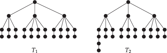
As a part of the computations, in order to support the Alavi, Malde, Schwenk, and Erdös conjecture [19], using the linear algorithm described above, it was verified that for all trees up to $25$ vertices, their independence polynomials are log-concave (and, consequently, unimodal), see also ref. [21]. All of the sudden, when the number of vertices of a tree reached $26$, there were found two trees having their independence polynomials unimodal but not log-concave. In other words, these trees are counterexamples to the conjecture due to Levit, Mandrescu [22], and Galvin [23].

The independence polynomials of the trees $T_1$ and $T_2$ defined in Figure 1 are as follows:

Figure 1.

Two trees with 26 vertices whose independence polynomials are not log-concave.

$$\begin{array}{r}I\left(T_1;x\right)=x^{14}+51x^{13}+2979x^{12}+18683x^{11}+55499x^{10}+100144x^9+\\ 121376x^8+103736x^7+63933x^6+28551x^5+9142x^4+2040x^3+\\ 300x^2+26x+1,\end{array}$$E9

where the non-log-concavity is demonstrated by the coefficient of $x^{13}$: ${51}^2<2979$, and

$$\begin{array}{r}I\left(T_2;x\right)=x^{14}+48x^{13}+2372x^{12}+15498x^{11}+48086x^{10}+90178x^9+\\ 112870x^8+98968x^7+62183x^6+28147x^5+9089x^4+2037x^3+\\ 300x^2+26x+1,\end{array}$$E10

where the non-log-concavity is demonstrated by the coefficient of $x^{13}$: ${48}^2<2372$.

6. Extensions of T1

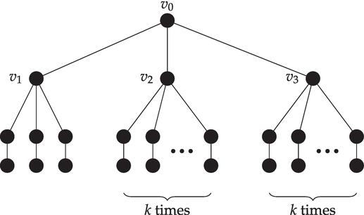
$T_1$ from Figure 1 is just an example belonging to an infinite family of trees such that their independent polynomials are not log-concave. Their structure, which we denoted 3,k,k structure, is described in the following and drawn in Figure 2:

• the tree has one center, denoted $v_0$ that is connected to three vertices $v_1,v_2,v_3$;

• $v_1$ is connected to $K_2\cup K_2\cup K_2$;

• $v_2$ is connected to $K_2\cup \dots \cup K_2$, $k$ times;

• $v_3$ is also connected to another $K_2\cup \dots \cup K_2$, $k$ times.

Figure 2.

An illustration of the 3,k,k structure of trees that have non-log-concave independence polynomials.

Lemma 6.1 All trees of the $3,k,k$ structure, where $k\ge 4$, have non-log-concave independence polynomials.

Proof: Let us compute the independence polynomial of a tree having $3,k,k$-structure, and choose $v_0$ to be the first vertex to remove from the graph.

$$I{\left(G\right)}_{v_0}=I\left(G-v_0\right)+x\cdot I\left(G-N\left[v_0\right]\right).$$E11

Expand the first term in that sum:

$$\begin{array}{{}I\left(G-v_0\right)=\left[{\left(2x+1\right)}^k+x{\left(x+1\right)}^k\right]\cdot \left[{\left(2x+1\right)}^k+x{\left(x+1\right)}^k\right]\\ \cdot \left[{\left(2x+1\right)}^3+x{\left(x+1\right)}^3\right]\\ ={\left[\sum _{i=0}^k\left(\begin{array}{c}k\\ i\end{array}\right){\left(2x\right)}^i+x\sum _{i=0}^k\left(\begin{array}{c}k\\ i\end{array}\right)x^i\right]}^2\cdot \left[{\left(2x+1\right)}^3+x{\left(x+1\right)}^3\right]\\ ={\left[x^{k+1}+\left(2^k+k\right)x^k+\left(k\cdot 2^{k-1}+\frac{k\left(k-1\right)}{2}\right)x^{k-1}+\cdots \right]}^2\\ \cdot \left[x^4+11x^3+15x^2+\cdots \right].\end{array}$$E12

We can divide the first term expression into three factors $A\cdot B\cdot C$ such that:

$$\begin{array}{{}A=\left[x^{k+1}+\left(2^k+k\right)x^k+\left(k\cdot 2^{k-1}+\frac{k\left(k-1\right)}{2}\right)x^{k-1}+\cdots \right];\\ B=\left[x^{k+1}+\left(2^k+k\right)x^k+\left(k\cdot 2^{k-1}+\frac{k\left(k-1\right)}{2}\right)x^{k-1}+\cdots \right];\\ C=\left[x^4+11x^3+15x^2+\cdots \right].\end{array}$$E13

Expand the second term in that sum:

$$\begin{array}{l}I\left(G-N\left[v_0\right]\right)=x\cdot {\left(2x+1\right)}^{2k+3}\\ =x\cdot \left[\sum _{i=0}^{2k+3}\left(\begin{array}{c}2k+3\\ i\end{array}\right){\left(2x\right)}^i\right]\\ =x\cdot \left[{\left(2k\right)}^{2k+3}+\cdots \right]\\ =2^{2k+3}{x}^{2k+4}+\cdots \end{array}$$E14

The highest exponent that one can reach is $2k+6$. We obtain it by taking the highest exponent from every factor, that is, from both factors $A$ and $B$_, we choose $x^{k+1}$, while from $C$ factor we choose $x^4$, so

$$x^{n+1}\cdot x^{k+1}\cdot x^4=X^{2k+6}$$E15

with the coefficient equal to $1$.

To calculate the coefficient of $x^{2k+5}$ we have three following options:

• multiply $\left(2^k+k\right)x^k$ from $A$, $x^{k+1}$ from $B$, and $x^4$ from $C$,

• multiply $x^{k+1}$ from $A$, $\left(2^k+k\right)x^k$ from $B$, and $x^4$ from $C$,

• multiply $x^{k+1}$ from $A$, $x^{k+1}$ from $B$, and $11x^3$ from $C$.

In such a way we obtain the following:

$$\left(2^k+k\right)x^k\cdot x^{k+1}\cdot x^4+x^{k+1}\cdot \left(2^k+k\right)x^k\cdot x^4+x^{k+1}\cdot x^{k+1}\cdot 11x^3=\left(2^{k+1}+2k+11\right)x^{2k+5}$$E16

with the coefficient equal to $2^{k+1}+2k+11$.

To calculate the coefficient of $x^{2k+4}$ we have six following options:

• multiply $x^{k+1}$ from $A$, $x^{k+1}$ from $B$, and $15x^2$ from $C$,

• multiply $x^{k+1}$ from $A$, $\left(2^k+k\right)x^k$ from $B$, and $11x^3$ from $C$,

• multiply $x^{k+1}$ from $A$, $\left(k\cdot 2^{k-1}+\frac{k\left(k-1\right)}{2}\right)x^{k-1}$ from $B$, and $x^4$ from $C$,

• multiply $\left(2^k+k\right)x^k$ from $A$, $x^{k+1}$ from $B$, and $11x^3$ from $C$,

• multiply $\left(2^k+k\right)x^k$ from $A$, $\left(2^k+k\right)x^k$ from $B$, and $x^4$ from $C$,

• multiply $\left(k\cdot 2^{k-1}+\frac{k\left(k-1\right)}{2}\right)x^{k-1}$ from $A$, $x^{k+1}$ from $B$, and $x^4$ from $C$.

Finally, we add the coefficient $2^{2k+3}$ from the second term. In such a way we obtain the following:

$$\begin{array}{l}{x}^{k+1}\cdot x^{k+1}\cdot 15x^2+x^{k+1}\cdot \left(2^k+k\right)x^k\cdot 11x^3+x^{k+1}\cdot \left(k\cdot 2^{k-1}+\frac{k\left(k-1\right)}{2}\right)\cdot x^4\\ +\left(2^k+k\right)x^k\cdot x^{k+1}\cdot 11x^3+\left(2^k+k\right)x^k\cdot \left(2^k+k\right)x^k\cdot x^4+\left(k\cdot 2^{k-1}+\frac{k\left(k-1\right)}{2}{x}^{k-1}\right)\\ \cdot x^{k+1}\cdot x^4+2^{2k+3}{x}^{2k+4}\\ =\left(2^{2k+3}+2^{2k}+\left(22+3k\right)2^k+2k^2+21k+15\right)x^{2k+4}.\end{array}$$E17

with the coefficient equal to $2^{2k+3}+2^{2k}+\left(22+3k\right)2^k+2k^2+21k+15$.

Thus the independence polynomial is as follows:

$$\begin{array}{r}I\left(G\right)=x^{2k+6}+\left(2^{k+1}+2k+11\right)x^{2k+5}+[2^{2k+3}+2^{2k}+\left(22+3k\right)2^k+2k^2+\\ 21k+15]x^{2k+4}+\cdots \end{array}$$E18

Now, let us prove the non-log-concavity in the $x^{2k+5}$ term of the independence polynomial:

$${\left(2^{k+1}+2k+11\right)}^2<1\cdot \left[2^{2k+3}+2^{2k}+\left(22+3k\right)2^k+2k^2+21k+15\right]$$E19

The left-hand side and the right-hand side are equal to $k\approx 3.5357$ so the left-hand side is smaller than the right-hand side from $k=4$ and above.

7. Extensions of T2

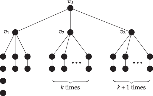
$T_2$ from Figure 1 is just an example belonging to an infinite family of trees whose independence polynomials are not log-concave. Let us denote the left sub-tree “3*.” Their structure, which we denote 3*,k,k + 1 structure is described in the following, and drawn in Figure 3:

Figure 3.

An illustration of the 3*,k,k + 1 structure of trees that have non-log-concave independence polynomial.

the tree has one center, denoted $v_0$ that is connected to three vertices $v_1,v_2,v_3$;

• $v_1$ is connected to $P_4\cup K_2\cup K_2$;

• $v_2$ is connected to $K_2\cup \dots \cup K_2$, $k$ times;

• $v_3$ is connected to another $K_2\cup \dots \cup K_2$, $k+1$ times.

Lemma 7.1. All trees of the $3^{\ast },k,k+1$ structure, where $k\ge 3$, have non-log-concave independence polynomials.

Proof: Let us compute the independence polynomial of a tree having $3^{\ast },k,k+1$ structure, and choose $v_0$ to be the first vertex to remove from the graph.

$$I{\left(G\right)}_{v_0}=I\left(G-v_0\right)+x\cdot I\left(G-N\left[v_0\right]\right)$$E20

Expand the first term in that sum:

$$\begin{array}{{}I\left(G-v_0\right)=\left[{\left(2x+1\right)}^{k+1}+x{\left(x+1\right)}^{k+1}\right]\cdot \left[{\left(2x+1\right)}^k+x{\left(x+1\right)}^k\right]\\ \cdot \left[{\left(2x+1\right)}^2\left(3x^2+4x+1\right)+x{\left(x+1\right)}^2\left(x^2+3x+1\right)\right]\\ =\left[\sum _{i=0}^{k+1}\left(\begin{array}{c}k+1\\ i\end{array}\right){\left(2x\right)}^i+x\sum _{i=0}^{k+1}\left(\begin{array}{c}k+1\\ i\end{array}\right)x^i\right]\cdot \left[\sum _{i=0}^k\left(\begin{array}{c}k\\ i\end{array}\right){\left(2x\right)}^i+x\sum _{i=0}^k\left(\begin{array}{c}k\\ i\end{array}\right)x^i\right]\\ \cdot \left[{\left(2x+1\right)}^2\left(3x^2+4x+1\right)+x{\left(x+1\right)}^2\left(x^2+3x+1\right)\right]\\ =\left[x^{k+2}+\left(2^{k+1}+k+1\right)x^{k+1}+\left(\left(k+1\right)\cdot 2^k+\frac{k\left(k+1\right)}{2}\right)x^k+\cdots \right]\\ \cdot \left[x^{k+1}+\left(2^k+k\right)x^k+\left(k\cdot 2^{k-1}+\frac{k\left(k-1\right)}{2}\right)x^{k-1}+\cdots \right]\\ \cdot \left[x^5+17x^4+36x^3+\cdots \right].\end{array}$$E21

We can divide the first term expression into three factors $A\cdot B\cdot C$ such that:

$$\begin{array}{{}A=\left[x^{k+2}+\left(2^{k+1}+k+1\right)x^{k+1}+\left(\left(k+1\right)\cdot 2^k+\frac{k\left(k+1\right)}{2}\right)x^k+\cdots \right],\\ B=\left[x^{k+1}+\left(2^k+k\right)x^k+\left(k\cdot 2^{k-1}+\frac{k\left(k-1\right)}{2}\right)x^{k-1}+\cdots \right],\\ C=\left[x^5+17x^4+36x^3+\cdots \right].\end{array}$$E22

Expand the second term in that sum:

$$\begin{array}{r}x\cdot I\left(G-N\left[v_0\right]\right)=x\cdot {\left(2x+1\right)}^{2k+3}\cdot \left(3x^2+4x+1\right)\\ =x\left(3x^2+4x+1\right)\cdot \left[\sum _{i=0}^{2k+3}\left(\begin{array}{c}2k+3\\ i\end{array}\right){\left(2x\right)}^i\right.]\\ =x\left(3x^2+4x+1\right)\cdot \left[{\left(2x\right)}^{2k+3}+\cdots \right]\\ =3\cdot 2^{2k+3}{x}^{2k+6}+\cdots \end{array}$$E23

The highest exponent that one can reach is $2k+8$. We obtain it by taking the highest exponent from every factor, that is, from factor $A$ we choose $x^{k+2}$, from factor $B$ we choose $x^{k+1}$, and while from $C$ factor we choose $x^5$, so

$$x^{n+2}\cdot x^{n+1}\cdot x^5=x^{2k+8}.$$E24

with the coefficient equal to $1$.

To calculate the coefficient of $x^{2k+7}$ we have three following options:

• multiply $x^{k+2}$ from $A$, $x^{k+1}$ from $B$, and $17x^4$ from $C$,

• multiply $x^{k+2}$ from $A$, $\left(2^k+k\right)x^k$ from $B$, and $x^5$ from $C$,

• multiply $\left(2^{k+1}+k+1\right)x^{k+1}$ from $A$, $x^{k+1}$ from $B$, and $x^5$ from $C$.

In such a way we obtain the following:

$$\begin{array}{r}{x}^{k+2}\cdot x^{k+1}\cdot 17x^4+x^{k+2}\cdot \left(2^k+k\right)x^k\cdot x^5+\left(2^{k+1}+k+1\right)x^{k+1}\cdot x^{k+1}\cdot x^5\\ =\left(2k+2^k+2^{k+1}+18\right)x^{2k+7}.\end{array}$$E25

with the coefficient equal to $2k+2^k+2^{k+1}+18$.

To calculate the coefficient of $x^{2k+6}$ we have six following options:

• multiply $x^{k+2}$ from $A$, $x^{k+1}$ from $B$, and $36x^3$ from $C$,

• multiply $x^{k+2}$ from $A$, $\left(2^k+k\right)x^k$ from $B$, and $17x^4$ from $C$,

• multiply $x^{k+2}$ from $A$, $\left(k\cdot 2^{k-1}+\frac{k\left(k-1\right)}{2}\right)x^{k-1}$ from $B$, and $x^5$ from $C$,

• multiply $\left(2^{k+1}+k+1\right)x^{k+1}$ from $A$, $x^{k+1}$ from $B$, and $17x^4$ from $C$,

• multiply $\left(2^{k+1}+k+1\right)x^{k+1}$ from $A$, $\left(2^k+k\right)x^k$ from $B$, and $x^5$ from $C$,

• multiply $\left(\left(k+1\right)\cdot 2^k+\frac{k\left(k+1\right)}{2}\right)x^k$ from $A$, $x^{k+1}$ from $B$, and $x^5$ from $C$.

Finally, we add the coefficient $3\cdot 2^{2k+3}$ from the second term. In such a way we obtain the following:

$$\begin{array}{r}{x}^{k+2}\cdot x^{k+1}\cdot 36x^3+x^{k+2}\cdot \left(2^k+k\right)x^k\cdot 17x^4+x^{k+2}\cdot \left(k\cdot 2^{k-1}+\frac{k\left(k-1\right)}{2}\right)x^{k-1}\cdot x^5\\ +\left(2^{k+1}+k+1\right)x^{k+1}\cdot x^{k+1}\cdot 17x^4+\left(2^{k+1}+k+1\right)x^{k+1}\\ \cdot \left(2^k+k\right)x^k\cdot x^5+\left(\left(k+1\right)\cdot 2^k+\frac{k\left(k+1\right)}{2}\right)x^k\cdot x^{k+1}\cdot x^5+3\cdot 2^{2k+3}{x}^{2k+6}\\ =\left(\frac{1}{2}k\left(4k+9\cdot 2^k+70\right)+53\cdot 2^k+13\cdot 2^{2k+1}+53\right)x^{2k+6}.\end{array}$$E26

with the coefficient equals to $\frac{1}{2}k\left(4k+9\cdot 2^k+70\right)+53\cdot 2^k+13\cdot 2^{2k+1}+53$.

Thus the independence polynomial is:

$$\begin{array}{l}I\left(G\right)=x^{2k+8}+\left(2k+2^k+2^{k+1}+18\right)x^{2k+7}+\\ \left[\frac{1}{2}k\left(4k+9\cdot 2^k+70\right)+53\cdot 2^k+13\cdot 2^{2k+1}+53\right]x^{2k+6}+\cdots \end{array}$$E27

Now, let us prove the non-log-concavity of the $x^{2k+7}$ term in the independence polynomial:

$${\left(2k+2^k+2^{k+1}+18\right)}^2<1\cdot \left[\frac{1}{2}k\left(4k+9\cdot 2^k+70\right)+53\cdot 2^k+13\cdot 2^{2k+1}+53\right].$$E28

The left-hand side and the right-hand side are equal to $k\approx 2.9251$ so the left-hand side is smaller than the right-hand side from $k=3$ and above.

8. Conclusions

In this chapter, we have presented a linear algorithm that uses dynamic programming to compute independence polynomials of trees. It allows us to check all trees up to $26$ vertices, to find $2$ trees of order $26$ with non-log-concave independence polynomials, and, finally, to construct two infinite families of trees having non-log-concave independence polynomials.

References

1.Gutman I, Harary F. Generalizations of the matching polynomial. Utilitas Mathematica. 1983;24:97-106
2.Hoede C, Li X. Clique polynomials and independent set polynomials of graphs. Discrete Mathematics. 1994;125:219-228
3.Chudnovsky M, Seymour P. The roots of the stable set polynomial of a clawfree graph. Journal of Combinatorial Theory, Series B. 2007;97:350-357. DOI: 10.1016/j.jctb.2006.06.001
4.Ball T, Galvin D, Hyry C, Weingartner K. Independent set and matching permutations. Journal of Graph Theory. 2022;(99):40-57. DOI: 10.1002/jgt.22724
5.Basit A, Galvin D. On the independent set sequence of a tree. The Electronic Journal of Combinatorics. 2021;28(3):#P3.23. DOI: 10.37236/9896
6.Stanley RP. Log-concave and unimodal sequences in algebra, combinatorics, and geometry. Annals of the New York Academy of Sciences. 1989;576:500-535
7.Brenti F. Log-concave and unimodal sequences in algebra, combinatorics, and geometry: An update, “Jerusalem Combinatorics’93”. Contemporary Mathematics. 1994;178:71-89
8.Brenti F. Unimodal, log-concave and Polya frequency sequances in Combinatorics. Memoris Amer, Math, Soc. 1990;108:729-756
9.Bender EA, Canfield ER. Log-concavity and related properties of the cycle index polynomials. Journal of Combinatorial Theory A. 1996;74:57-70
10.Boros G, Moll VH. A sequence of unimodal polynomials. Journal of Mathematical Analysis and Applications. 1999;237:272-287
11.Brown JI, Colbourn CJ. On the log-concavity of reliability and matroidal sequences. Advances in Applied Mathematics. 1994;15:114-127
12.Dukes WMB. On a unimodality conjecture in matroid theory. Discrete Mathematics and Theoretical Computer Science. 2002;5:181-190
13.Levit VE, Mandrescu E. On unimodality of independence polynomials of some well-covered trees. Discrete Mathematics and Theoretical Computer Science. 2003;4:237-256
14.Schwenk AJ. On unimodal sequences of graphical invariants. Journal of Combinatorial Theory B. 1981;30:247-250
15.Hamidoune YO. On the number of independent k-sets in a claw-free graph. Journal of Combinatorial Theory B. 1990;50:241-244
16.Chudnovsky M, Seymour P. The roots of the independence polynomial of a claw-free graph. Journal of Combinatorial Theory, Series B. 2007;97:350-357
17.Beaton I, Brown JI. On the unimodality of domination polynomials. Graphs and Combinatorics. 2022;38:90. DOI: 10.1007/s00373-022-02487-x
18.Horrocks DGC. The numbers of dependent k-sets in a graph are log concave. Journal of Combinatorial Theory, Series B;84(2002):180-185. DOI: 10.1006/jctb.2001.2077
19.Alavi Y, Malde PJ, Schwenk AJ, Erdös P. The vertex independence sequence of a graph is not constrained. Congressus Numerantium. 1987;58:15-23
20.Yosef R, Mizrachi M, Kadrawi O. On unimodality of independence polynomials of trees. 2021. Available from: https://arxiv.org/pdf/2101.06744v3.pdf. [Accessed: December 8, 2022]
21.Radcliffe AJ. Personal communication (mentioned in Ball T, Galvin D, Hyry C, Weingartner K. Independent set and matching permutations. Journal of Graph Theory. 2022;(99):40-57.)
22.Levit VE, Mandrescu E. Very well-covered graphs with log-concave independence polynomials. Carpathian J. Math. 2004;20:73-80
23.Galvin D. REGS 2011. Available from: https://faculty.math.illinois.edu/west/regs/stasetseq.html. [Accessed: December 8, 2022]
24.Levit VE, Mandrescu E. The independence polynomial of a graph - a survey. In: Proceedings of the 1st International Conference on Algebraic Informatics. Thessaloniki: Aristotle University of Thessaloniki; 2005. pp. 231-252
25.Arocha JL. Propriedades del polinomio independiente de un grafo. Revista Ciencias Matematicas. 1984;3:103-110
26.Ferrin GM. Independence polynomials [Thesis]. Columbia, South Carolina: University of South Carolina; 2014
27.Bodlaender HL. A linear time algorithm for finding tree-decompositions of small treewidth. SIAM. 1996;25:1305-1317
28.Tittmann P. Graph Polynomials: The Ethernal Book. Productivity Press; 2021
Written By
Ohr Kadrawi, Vadim E. Levit, Ron Yosef and Matan Mizrachi
Submitted: 15 December 2022Reviewed: 15 January 2023Published: 07 March 2023
Open access peer-reviewed chapter