Borderless Optimization Method Genetic Algorithm

Abstract

Genetic algorithms, a stochastic research method, are Darwin’s “survival of the best.” Development of biological systems based on the principle of “survival of the fittest” emerged with the adaptation of the process to the computer environment. In genetic algorithms, processes executed are stored in computer memory similar to natural populations performed on units. Today, there are many linear and nonlinear solutions for optimization problems. The method has been developed. Designing optimization problems with these method variables is assumed to be continuous. But this acceptance does not always valid. In some problems, there are too many design variables and constraints for traditional optimization in solving such problems. The use of this method sometimes gives erroneous results or the solution time is too long. Since genetic algorithms are an intuitive method, a given may not find the optimum result for the problem. However, it optimizes the problems that cannot be solved by known methods or the solution time of the problem is too long. Initial nonlinear optimization genetic algorithms applied to the problems of traveling salesman, workshop scheduling, and syllabus preparation, such as complex optimization problems, have been successfully implemented.

1. Introduction

Genetic algorithms, a stochastic research method, emerged by adapting the development process of biological systems to the computer environment. Operations using genetic algorithms are performed on units stored in computer memory, similar to natural populations. Today, many linear or nonlinear methods have been developed for the solution of optimization problems. In these problems, it is accepted that the design variables are continuous. However, this acceptance is not always valid. Due to a large number of design variables and constraints in some problems, the use of traditional optimization methods in solving such problems sometimes gives erroneous results or the solution time is too long. Genetic algorithms may not find the optimum result for a given problem. However, it gives values very close to the optimum values for problems that cannot be solved by known methods or whose solution time increases exponentially with the solution of the problem. Genetic algorithms have been successfully applied to complex optimization problems, such as traveling salesman, workshop planning, and curriculum preparation. The basic principles of genetic algorithms were first introduced by Holland [1]. The discovery of the crossover operator by Holland played a major role in the development of genetic algorithms. In his studies, Holland was driven by the idea of developing species that can adapt very well to their environment with the effect of sexual intercourse, reproduction, and natural selection. The first work in the literature on genetic algorithms is John Holland’s Machine Learning. The study by David E. Goldberg, a student of Holland, who was later influenced by this study, on the control of gas pipelines proved that genetic algorithms can have practical uses. The problems for which genetic algorithms are most suitable are those that cannot be solved by traditional methods or whose solution time increases exponentially with the size of the problem. Until today, it has been tried to solve problems in different fields using genetic algorithms. Some of these fields of study are optimization, automatic programming, machine learning, economics, immune systems, population genetics, evolution, and learning and social systems.

2. Structure and basic principles of genetic algorithms

In the first step of the genetic algorithms, an initial collection of subsets of all possible solutions is obtained. Each member of the community is coded as an individual. Each individual is biologically equivalent to a chromosome. Every individual in the community has a fitness value. The fitness value determines which individual will move to the next community. The strength of an individual depends on his/her fitness value, and a good individual has a high fitness value if it is a maximization problem and a low fitness value if it is a minimization problem (Table 1) [2].

Profile number	Profile section
1	IPE200
2	IPE220
3	IPE240
4	IPE270

Table 1.

Profile numbers and codes of these profiles.

Genetic algorithms used in solving any problem consist of the following components:

1. Representation of individuals forming the community as a sequence (“chromosome”).

2. Creation of the startup community.

3. Determining the eligibility of individuals and establishing the evaluation function.

4. Genetic operators for obtaining new populations.

5. Control variables (probabilities of crossover and mutation operators and the number of members in the ensemble).

3. Coding

The most important feature that distinguishes genetic algorithms from other methods is the use of codes representing these variables instead of variables. The first step in applying the genetic algorithm to any problem is to choose the most appropriate coding type for the problem. 2.4.1 binary coding.

3.1 Binary coding

In binary coding, each individual consists of the numbers 0 and 1 (Table 2). Chromosome length of the individual should be selected to include all points between the lower and upper limits of the parameter or variables. For a function with more than one variable, the chromosome length is equal to the sum of the chromosome lengths determined for each variable [1].

Number	1. rod				2. rod				3. rod			4. rod					5. rod
Prf; number	1	2	3	4	1	2	3	4	1	2	3	4	1	2	3	4	1	2	3	4
Code	1	2	3	4	1	2	3	4	1	2	3	4	1	2	3	4	1	2	3	4

Table 2.

Code of a random individual in binary coding type.

Although binary coding is a very common type of coding, it has some drawbacks. In multivariate function optimizations, the individual length obtained depending on the lower and upper limits of the variables is very large. Also traveling salesman scheduling etc. In complex optimization problems, binary coding does not fully represent the design space. For this reason, in addition to binary coding, real number coding and permutation coding types are also used.

3.2 Permutation coding

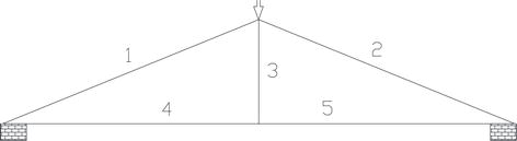
In permutation coding, the chromosome length is equal to the number of design variables. Permutation coding type is especially preferred in problems where design variables consist of more than one subvariable. The superiority of this coding type in shape optimization is illustrated with a simple example (Example 2.1.). In this coding type, the codes of the design variables consist of randomly selected numbers between 1 and the number of design variables (Table 3) (Example 1). In the problem of “optimizing sizing of the truss in Figure 1,” the code of any individual to be included in the starting group is shown separately as permutation coding and binary coding.

	1.rod	2.rod	3.rod	4.rod	5. rod
Code	3	1	4	2	3

Table 3.

Code of a random individual in permutation coding type.

Figure 1.

Truss beam model is used to explain coding types.

4. Creating the initial population

Another important feature that distinguishes genetic algorithms from other methods is that it performs a search within a community of points, not point-to-point [1]. Therefore, the first step of the genetic algorithm is the creation of the initial population. In a problem with variable number L, it is recommended that the number of elements in the initial collection is between 2 L ∼ and 4 L [3]. The initial population is simply randomly generated. However, especially in limited optimization problems, as a result of the random creation of the initial population, unsuitable solutions that do not meet the boundaries emerge. To eliminate this situation, it is to benefit from the heuristic methods developed for the problem. There are various studies in the literature that use heuristic methods in the creation of the initial community. For example, Grefenstette used gredgreedyristics in the traveling salesman problem, Kapsalis et al. used the minimum tree approach in the Steiner tree problem, Thiel and Vass used the addition-subtraction heuristics in the 0−1 backpack problem, and Chen et al. used the Campbell Dubek-Smith, and Dannenbrigt heuristics for the scheduling problem [4].

5. Evaluation

In each generation, the fitness values of the individuals in the community are calculated with an evaluation function. The fitness value plays a role in determining which candidate solutions from the existing community will be used to obtain new candidate solutions that will form the next community. The evaluation function used in genetic algorithms is the objective function of the problem. However, in some problems, objective functions may be limited by design variables. In this case, objective functions constrained by design variables should be converted to unconstrained objective functions independent of design variables with two transformations [5].

In the first transformation, the constrained objective function f(s) is transformed into the unconstrained objective function Ø(s) by applying the following transformation. Error functions are used in this transformation.

$$\mathrm{Ø}\left(\mathrm{s}\right)=\left[\mathrm{f}\left(\mathrm{s}\right)+\mathrm{R}.\sum \mathrm{\Phi }\left(\mathrm{Z}\right)\right]$$E1

If Z > 0 ise Φ(Z) = Z2

$$\text{If}\mathrm{Z}\le 0\mathrm{ise}\mathrm{\Phi }\left(\mathrm{Z}\right)=0$$E2

In the second transformation, the unconstrained objective function Ø(s) is transformed into the fitness function F(s).

$$\mathrm{F}\left(\mathrm{s}\right)=\mathrm{Ø}max-[\mathrm{f}\left(\mathrm{s}\right)+\mathrm{R}.\sum \mathrm{\Phi }(\mathrm{gj}\left(\mathrm{x}\right)]\mathrm{F}\left(\mathrm{s}\right)=\mathrm{Ø}max-\mathrm{Ø}\left(\mathrm{s}\right)$$E3

f(s): Constrained objective function.

R: Predetermined error coefficient (R = 10,100…).

Φ(Z): Error function.

Ø(s): Unconstrained objective function.

Ø max: The maximum value of the unconstrained objective function.

F(s): Fitness function.

The fitness values of individuals are calculated from Eq. (3) [5]. Then, according to these fitness values, individuals to be used in the next stage are determined by any of the following methods.

When proportional selection methods are used in minimization problems, it is not possible to directly use the objective function to calculate the fitness values because these selection mechanisms are concerned with maximizing fitness. One method used to transform minimization problems into maximization problems is to multiply the objective function of the minimization problem by (−1). However, this method is not used in genetic algorithms due to the condition that the fitness values are positive. A minimization problem solved by genetic algorithms is transformed into a maximization problem by subtracting the objective function value of the problem from a large value determined at the beginning [1].

6. Selection methods

After the initial community is formed, in each generation, the members of the new community are selected from among the members of the existing community through a selection process. Individuals with a high fitness value have a high probability of acquiring new individuals. This operator performs natural selection artificially. The fitness of natural communities is determined by the ability of individuals to withstand the barriers of growth and reproduction. The various selection methods used are summarized below.

6.1 Proportional selection methods

6.1.1 Selection method with roulette wheel

The simplest selection method used in genetic algorithms is the Roulette Wheel method. In this method, the circle is divided into N equal spacing. In the circle spacings represents the elements. And the width of this interval is equal to the probability that this individual will be selected. In this case, the sum of the gap widths in the circle is equal to 1. During the selection phase, the circle is turned N times. In each turn, the individual indicated by the roulette dial is copied to the new community [1].

Although the roulette wheel method is simple, it has a stochastic error. In the new population, there is a difference between the expected number of copies of each individual and the number of copies that occur. In the next generations, this error increases and the search continues in many different directions than what was predicted theoretically. This event can cause generations to converge prematurely.

6.1.2 Stochastic ascending selection method

In this method, first of all, the expected copy number (mi) of the sequences in the ensemble is calculated. An integer copy of the expected value of each individual is registered in the new community. If the ensemble width is not reached, the fractional parts of the expected values are used with probability to fill the ensemble. There are two approaches to using fractional parts. The first approach is a choice without replacement. In this approach, the fractional part is taken into account as the probability value. For example, if the expected value of a copy of an individual is 1.5, a copy of this individual is included in the new community. The probability of the other copy being in the community is 50%. The other approach is choice by substitution. This approach uses a roulette wheel. The fractional parts are used to determine the intervals in the circle [4].

6.1.3 Stochastic universal selection method

This method is similar to the roulette wheel selection method. The most important difference is that the outer parts of the circle are divided into equal parts. The number of these parts is equal to the width of the ensemble. During the selection phase, the circle is rotated once. The copy number of an individual is determined by the number of pieces on the outside of the circle. In this case, the number of pieces falling on the weighted weight of an individual in the circle gives the number of copies of that individual [1].

6.1.4 Sequential selection method

The operation of this mechanism is summarized as follows. First of all, individuals in the community are ranked according to their fitness values from best to worst. The copy number is assigned to individuals with the help of a decreasing function. The most common assignment function used is linear. The copy numbers assigned with the help of a function are used to create the new community. At this stage, a new community is obtained by using one of the proportional selection mechanisms. It is stated that the number of copies of the best individual should be between 1 and 2 to control the election pressure in a community. The sequential selection mechanism has two major advantages. The first is that the scaling functions that should be used for the reasons explained do not need to be used in this selection mechanism. The second is to take the fitness values equal to the objective function values in minimization problems. This does not apply to proportional selection mechanisms.

6.1.5 Tournament selection method

In this mechanism, which has the advantages of the sequential selection mechanism, a group of individuals is randomly selected from the community. The individual with the best fitness value in this group is copied to the new community. This process is continued until the community width is reached. Generally, the group width is taken as two. However, it is also possible to increase this number [1].

6.1.6 Equilibrium selection method

The functioning of this mechanism is different from the others. In the methods described, firstly, a new population is obtained by selecting individuals from the existing population, and new individuals are obtained by applying genetic operators to the obtained population. The new individuals obtained are taken into the new community by replacing them with the individuals used to create them. In this method, genetic operators are applied to one or two individuals selected using the linear sequential selection method, and a new population is formed by replacing the new individuals obtained with the individuals with the lowest fitness value in the existing population.

6.1.7 Developed back-controlled selection operator (BCSO)

The selection process in existing selection operators is performed among individuals composing the population in the same generation. In these selection operators, the selection is carried out according to the fitness values ​​of each individual. The fitness value of the individual in the existing generation is compared with the fitness value in the same generation. The BCSO differs from existing selection operators because the fitness value of the individual is compared with the fitness value in the previous generation. If the fitness value of the individual is more than the one in the preceding generation, this individual would keep their own position. Otherwise, if the fitness value of the same individual is less than or equal to the fitness value in the preceding generation, this individual would be discarded from the population. The individual would be copied to the population in the preceding generation to replace this individual.

7. Crossover operator

Crossover is a search operator that provides access to similar but unexplored regions of the search space by exchanging information between different solutions. With the crossover operator, two different individuals, which will give new points in the search space, are obtained by interchanging certain parts of two randomly selected individuals from the community. One-point, two-point, and uniform crossover methods are widely used in the literature.

7.1 One-point crossover operator

In this operator, the crossover point is randomly chosen between 1 and L-1. In two matched individuals, the segments after this cut-off point are replaced and two new individuals are obtained. In Table 4, a point crossover operator was applied to the parts of the individuals after the fifth site.

1	0	1	1	0	1	0	1		0	1	1	1	0	0	1	1
Parent 1									Child 1
1	1	1	1	0	0	1	1		0	0	1	1	0	1	0	1
Parent 2									Child 2

Table 4.

One-point crossover operator.

7.2 Two-point crossover operator

The only difference between these crossover operators from the one-point crossover operator is that two different intercept points are chosen randomly between 1 and L⁻¹. New individuals are obtained by relocating the regions of matched individuals between these breakpoints. An example of a two-point crossover performed at sites between the third and sixth cut points is given (Table 5).

1	0	1	1	0	1	0	1		1	0	1	1	0	0	0	1
Parent 1									Child 1
1	1	1	1	0	0	1	1		1	1	1	1	0	1	1	1
Parent 2									Child 2

Table 5.

Two-point crossover operator.

7.3 Uniform crossover operator

In this operator, a random individual is temporarily created in binary order to be used in uniform crossover. The chromosome length of this individual is equal to the chromosome lengths of the other individuals in the community and n of the chromosome of the transient individual. If the code of the site is 0, the first new individual is n. The code of the 1st old individual on the site is the n of the second new individual. The code of the 2nd former individual will be used on the site, likewise, the chromosome of the temporary individual n. If the code of the site is 1, the n. 2. the old individual’s code on the site is the n of the second new individual. The code of the 1st former individual will be used on the site. An example of uniform crossover is given in Ref. [6]. The fact that the number of temporary individuals to be used in this crossover method is equal to the number of pairs to be crossed over in the community and that these temporary individuals are not similar to each other is effective in the efficiency of the crossover operator (Table 6).

0	1	1	0	0	1	0	0
Temporary array
1	0	1	1	0	1	0	1		1	0	0	1	0	0	0	1
Parent 1									Child 1
1	0	0	1	0	0	1	0		1	0	1	1	0	1	1	1
Parent 2									Child 2

Table 6.

Uniform crossover.

8. Mutation operator

When working on a limited population, there is a possibility that some genetic information in the population will be lost prematurely after a while. All the genes that make up a chromosome can be the same. It is not possible to replace such a chromosome with the crossover operator. In this case, the gene in the randomly selected site on the chromosome is modified by interfering with the chromosomes that make up the community at a certain rate [1] (Table 7). It is recommended to take the mutation rate between 0.0001 and 0.05 [7]. We have the opportunity to produce individuals with high fitness values, which we cannot produce by crossover, by mutation. In addition, individuals with high fitness are at risk of being spoiled as a result of mutation [8].

First-person before mutation								Second-person before mutation
0	1	0	1	0	1	1		0	1	0	1	0	0	1
0	1	0	1	0	0	1		0	1	0	1	0	1	1
First-person after mutation								Second-person after mutation

Table 7.

Mutation of two different individuals with binary code.

9. Factors affecting the performance of genetic algorithm

Mutation rate: If the chromosomes start to resemble each other and are still far from the solution points, the mutation process is the only way to get the genetic algorithm out of its jam. However, giving a high value will prevent the genetic algorithm from reaching a stable point.

The number of crossover sites: Normally, crossover is performed at a single point, but research has shown that multipoint crossover is very useful in some problems.

How to evaluate the individuals obtained as a result of the crossover: It is sometimes important whether the two individuals obtained will be used at the same time.

Whether the generations are disjointed: Normally, each generation is created entirely dependent on the previous generation. In some cases, it may be useful to create the new generation with the old generation together with the individuals of the new generation obtained so far.

How the coding representation is made: However, it is not clear enough how it is a point that affects the performance of the genetic algorithm. Binary coding, permutation coding, and real number coding are the most common coding methods.

How the success evaluation is done: A poorly written evaluation function can prolong the runtime or cause the solution to never be reached.

10. Control parameters

In a genetic algorithm, there are three different control parameters: the size of the initial population, the crossover rate, and the mutation rate. The performance of a genetic algorithm is very dependent on the value of these parameters. Therefore, before applying genetic algorithms to a problem, the best combination of parameters must be determined.

10.1 The size of the starting group (N)

The size of the initial population is related to the convergence of the algorithm. The performance of the genetic algorithm decreases when the size of the initial population is small, because small heaps are insufficient to sample the search space and cause untimely convergence. The large initial population, on the other hand, increases the efficiency of the search, as it provides a very good sampling of the solution space and prevents premature convergence. However, when the size of the initial population is large, the evaluation of the sequences at each iteration increases the runtime and convergence occurs very slowly.

10.2 Crossover ratio

The crossover ratio controls the frequency of use of the crossover operator. In each new stack, the crossover operator is applied to Pç.N arrays. The high crossover rate realizes community variability quickly. A low-crossover rate causes the search to be very slow.

10.3 Mutation rate

Each element of each sequence in the new heap obtained by the selection process undergoes random changes with a probability equal to the Pm mutation rate. Since the high mutation rate turns the search made by the genetic algorithm into a random search, a low mutation rate should be preferred.

11. Conclusions

Genetic algorithms are one of the methods used as an alternative to traditional methods in solving optimization problems and are widely used in topology, shape, and size optimizations in the field of engineering. Genetic algorithms start with a population called the initial population, rather than a single individual that is likely to be the optimum solution to the solution of any optimization problem. In solving optimization problems with genetic algorithms, the risk of being caught in local optimum traps is less than in traditional optimization methods. Genetic algorithms use unconstrained objective functions in solving optimization problems. The use of unconstrained objective functions also enables the solution of multivariate optimization problems. Genetic algorithms, which are not an ordinary research technique, enable the discovery of new combination that comes with higher fitness values in each generation by using the best objective function and best fitness function values. Genetic algorithms can also be applied to optimization problems in cases where the design space is not discontinuous and convex, and where the design variables are mixed, continuous, and discontinuous. In classical optimization methods, it is necessary to find the first derivatives of the objective functions. In some complex optimization problems, finding the derivative of the objective function is either very difficult or impossible. In the use of genetic algorithms in optimization problems, there is no need for derivatives of objective functions, unlike classical optimization methods.

References

1.Goldberg DE. Genetic Algorithms İn Search, Optimization and Machine Learning. Addison-Wesley Publishing Company, Inc; 1989
2.Michalewicz Z. Genetic Algorithms+Data Structures=Evolutions Programs. Berlin Heidelberg, New York, USA: Springer-Verlag; 1996
3.Turgut P. Determination of Live Load Combinosomes in Structures by Genetic Algorithms. Ankara, Turkey: Fırat University, Institute of Science and Technology; 1995
4.Altiparmak F. Topological Optimization of Communication Networks with Genetic Algorithms. Ankara, Turkey: Gazi University Institute of Science and Technology; 1996
5.Rao S. Engineering Optimization. Wiley Eastern Limited, Publishers And New Age İnternational Publishers, Ltd.; 1995
6.Syswerda G. Uniform crossover in genetic algorithms. In: Third International Conference on Genetic Algorithms. 1989. pp. 2-9
7.Erbatur F, ve Hasancebi O. Structural Design Optimization Using Genetic Algorithm, Department Of Civil Engineering Middle East Technical University, Uğur Ersoy symposium. 1999
8.Holland JH. Adaptation in Natural and Artificial Systems. Ann Arbor: The University of Michigan Press; 1975
Written By
Mustafa Kaya
Submitted: 27 September 2022Reviewed: 08 October 2022Published: 26 July 2023
Open access peer-reviewed chapter