Do the Interest Rates Really Relate to Economic Growth? The Case of Greece

Abstract

We empirically investigate the relationship between the economic growth and various monetary variables, focusing on the Greek economy. Using monthly data on the Industrial Production Index (IPI) as a proxy for economic growth, along with 10-year bond yields, 10-year bond spreads, and 3-month and 12-month interest rates, we aim to incorporate them into a multivariate GARCH-DCC econometric framework. Specifically, we examine the DCCs’ behavior during the memoranda period, pandemic period and a stable period. Our main result is that in almost all cases, the economic growth is not affected by changes in interest rates, the spread or the bond yield. Only during the pandemic period seems to be a negative relationship between the spread and bond in relation to IPI, while the 3-months rate and IPI follow a different pattern. This adds to recent doubts about the prevailing conduct of monetary policy and common theoretical models (e.g., lowering interest rates may have no effect, when trying to stimulate the economy). These results provide crucial implications for policymakers and highlight the need for some form of policy coordination among central banks.

1. Introduction

The main aim of this research is to examine the relationship between economic growth and various monetary variables, such as 3-months and 12-months interest rates and 10-years bond spread and yield. For establishing a suitable monetary policy, it is essential to know if there is a relevant interdependence in data between gross domestic product and interest rates. Furthermore, we focus on Greece, a European Union country that tarnished the last decade by multiple crises (i.e., adjustment programs, pandemic and energy crisis). In most cases, the cost of borrowing for both individuals and businesses has an impact on economic growth. The level of interest rates affects economic growth and economic activity, but the relationship between the two is also affected by other factors in a more complex way. Factors such as inflation, monetary policies and inflation have an important role and define the magnitude of this impact. Moreover, the effects of interest rates on growth may vary between crisis periods.

Prior literature has empirically investigated the issue, with mixed results. The seminal work of Lee and Werner [1] examined the relationship between interest rates and economic activity in 19 economies with a sample spanning from 1955:01 to 2015:03. In their empirical analysis, multivariate GARCH-DCC models and Granger causality tests are employed. Their main results indicate that interest rates are not negatively correlated with economic growth and do not “Granger” cause growth. Also, they found that lower interest rates may be counter-productive when trying to stimulate the economy since interest rates capture investors’ beliefs for economic growth in the near future. This result leads the term spread to be able to forecast economic growth (see, [2]).

The results of Ferreira et al. [3] indicate that Economic Sentiment Indicator, an indicator introduced by the European Commission, can be explained by European yield of 97,5%. This confirms that yield spreads forecast economic growth and reflect investors’ expectations. On the contrary, a study based on a dynamic model for yields and GDP indicates that short-term rate predicts more accurately than term spreads [4]. These findings confirm that spreads were a good indicator of economic growth, but this ability has reportedly declined [5].

Liu et al. [6] proposed a new theoretical link between falling interest rates, increasing market concentration, and declining productivity growth. The framework is particularly pertinent to antitrust policy in an era of historically low-interest rates. While conventional models suggest that lower interest rates should stimulate productivity-enhancing investment, this study identifies an opposing strategic effect at very low-interest rates. In industries where firms compete both in terms of price and investment in productivity-enhancing technology, market leaders respond more aggressively to lower interest rates compared to followers. This amplified response leads to greater market concentration and eventually lower aggregate productivity growth. Also, the model provides an explanation for declining productivity growth, the rising share of profits, and increased market concentration.

Shaukat et al. [7] implement dynamic panel data methodology to analyze data from 1996 to 2015 for 38 countries. The results show that low-interest rates are beneficial for economic growth. Another study by Udoka and Anyingang [8] shows that high-interest rates result in lower GDP, implying that there is an inverse relationship between interest rates and economic growth.

According to Del Negro et al. [9], safe and liquid assets have declined in the last two decades, especially in advanced economies. Also, safety and liquidity convenience yield has increased whereas economic growth across all countries has declined, resulting in closer trends in real interest among advanced economies.

On public debt and low-interest rates, Blanchard [10] states that public debt does not necessarily lead to fiscal cost. In the case of the US, interest rates should be lower than economic growth rates to be a safe option, otherwise will result in debt rollovers. Moreover, the author advocates that welfare costs are lower than expected in the case of public debt, whereas marginal product of capital may not be accurately calculated. Finally, there can be multiple equilibria in investor markets, indicating that high public debt would not be beneficial for the economy.

Albu and Albu [11] conducted an empirical study using wavelet analysis confirming the relationship between public debt and economic growth. Their results indicate a strong negative relationship between public debt and economic growth.

Several studies have investigated interest rates and monetary policy by implementing a wavelet approach, giving the advantage of examining the factors both in long and short term. Hayat et al. [12] conducted research on Pakistan investigating the effect that inflation has on an interest rate of output growth. Their results indicate that the causal relationship in short and medium run is unidirectional and bidirectional in the long run. Crowley and Hudgins [13] using a discrete wavelet analysis indicate that monetary policy is more effective on economic growth when it targets inflation or economic growth. Examining the transmission channels of monetary policy in the US, Odo and Bosniak [14] conclude that during periods of financial uncertainty, investment and bank lending channels are the most effective. On the contrary, during low volatile periods, money and credit channels have more impact.

We contribute to the existent literature in the following aspects: Firstly, we extend the work of Lee and Werner [1], using the Athens Stock Exchange (ASE) Index and the Economic Sentiment Indicator (ESI) as explanatory variables in the return equation. In addition, we employ data with monthly frequency in contrast to quarterly data, so we can observe in more detail the economic and political impact on economic growth. Secondly, as far as the authors are aware, this is the first study to employ the wavelet coherence analysis on this dataset. Finally, yet importantly, we investigate the co-movement between economic growth and the other variables during the global financial crisis (GFC), European sovereign debt crisis (ESDC), and the COVID-19 pandemic crisis.

The paper is organized as follows: Section 2 presents the data and preliminary analysis. Section 3 analyzes the methodology. Section 4 represents the empirical results. Section 5 concludes.

2. Data and preliminary analysis

The data derived from Eurostat and the sample covers a period from January 2000 to July 2022, using 270 monthly observations. We use the industrial productivity index as a proxy for GDP, the 3-months interest rates, the 12-months interest rates, the 10-year Treasury bond, and the 10Y Greek spread defined as the difference between the German and Greek bond (all in first differences). Also, we use the Economic Sentiment Indicator (ESI) and the general index of the Athens Stock Exchange (ASE).

The Industrial Production Index’s growth rate is often used as a proxy for real GDP growth. Several studies that require a monthly frequency for GDP data adopt this approach.¹ The reason for choosing the month-to-month growth rate is that for short-term forecasts, this analysis is tracking closer the cyclical changes than the year-to-year percentage change which depends on what happened 1 year before. Furthermore, we use the percentage calculation of growth rate in contrast to logarithmic difference because the times series of interest rates have negative values.

Table 1 presents the summary statistics of variables. We can observe that the average level of industrial productivity index is 121.15. The maximum value is 151.89 (August 2000), while the minimum value is 94.7 (June 2015), indicating the fragility of Greek economy and the effect of capital controls during that period. The 10-year treasury bond is on average 4.19 with median 1.75 and we observe an extreme range (0.59–29.24). Similar results can be observed for the spread which is a measure of country risk. The ESI is on average 100.2 with maximum value 119.9 and minimum 79.9. Finally, the 3-months interest rate has mean 1.44 and the 12-months has mean 1.68. Also, both interest rates have negative minimum value and similar standard deviation. Furthermore, Jarque-Bera statistic rejects normality at the 1% level for all variables. For this reason, the estimation of multivariate BEKK model is based on t-student distribution.

	Industrial Production Index	Greek Government Bond 10Y	Spread	Interest Rate 3-Months	Interest Rate 12-Months	Economic Sentiment Indicator	Greek Stock Market (ASE)
Mean	121.15	6.47	4.19	1.44	1.68	100.20	1882.80
Median	115.53	5.07	1.754	0.85	1.37	102.10	1416.80
Maximum	151.89	29.24	27.38	5.11	5.39	119.90	5334.50
Minimum	94.70	0.59	0.12	−0.58	−0.50	79.00	516.710
Std. Dev.	17.70	4.90	5.29	1.79	1.77	9.98	1316.45
Skewness	0.20	2.19	1.99	0.59	0.50	−0.30	0.92
Kurtosis	1.40	8.74	7.46	1.97	1.98	2.15	2.69
Jarque-Bera	30.8***	589.7***	404.9***	27.6***	23.12***	12.29**	39.76***
Prob.	0.0000	0.0000	0.0000	0.0000	0.0000	0.0021	0.0000

Table 1.

Descriptive statistics of the series.

^***

represent statistical significance at the 1% levels.

^**

represent statistical significance at the 5% level.

The stationarity hypothesis is a requirement for the BEKK model, causality test and wavelet coherence analysis. Table 2 presents the stationarity test for all variables. Both Augmented Dickey-Fuller and Phillips-Perron tests indicate that the variables are I(0).

Panel A: Augmented Dickey-Fuller Test
Variable	t-statistic	prob.
Industrial Production Index	−13.45	0.0000
Diff.(Industrial Production Index)	−11.86	0.0000
Government Bond 10Y	−13.07	0.0000
Diff.(Government Bond 10Y)	−13.50	0.0000
Spread	−12.60	0.0000
Diff.(Spread)	−14.87	0.0000
Interest Rate 3-Months	−11.02	0.0000
Diff.(Interest Rate 3-Months)	−14.00	0.0000
Interest Rate 12-Months	−15.57	0.0000
Diff.(Interest Rate 12-Months)	−21.27	0.0000
Economic Sentiment Indicator	−15.12	0.0000
Diff.(Economic Sentiment Indicator)	−11.07	0.0000
Greek Stock Market (ASE)	−15.61	0.0000
Diff.(Greek Stock Market (ASE))	−13.90	0.0000
Panel B: Phillips-Perron Test
Variable	Adj. t-statistic	prob.
Industrial Production Index	−28.32	0.0000
Diff.(Industrial Production Index)	−172.80	0.0001
Government Bond 10Y	−13.29	0.0000
Diff.(Government Bond 10Y)	−70.79	0.0001
Spread	−12.90	0.0000
Diff.(Spread)	−74.47	0.0001
Interest Rate 3-Months	−11.14	0.0000
Diff.(Interest Rate 3-Months)	−38.49	0.0001
Interest Rate 12-Months	−15.57	0.0000
Diff.(Interest Rate 12-Months)	−228.27	0.0001
Economic Sentiment Indicator	−15.13	0.0000
Diff.(Economic Sentiment Indicator)	−72.25	0.0001
Greek Stock Market (ASE)	−15.69	0.0000
Diff. (Greek Stock Market (ASE))	−105.95	0.0001

Table 2.

Stationarity tests of the series.

Notes: The critical values for both tests at 1%, 5% and 10% significant levels are −3.45, −2.87 and − 2.57, respectively. The models include intercept, while for ADF model the selection of lag length performed via AIC and SIC (maximum lags 4). Regarding the PP test, the Bartlett kernel-based estimator of spectral density was adopted, while the bandwidth parameter was selected via Newey-West procedure. The p-values are calculated according to MacKinnon one-sided p-values.

3. Methodology framework

The scalar BEKK model proposed by Engle and Kroner [17] can be described from the following equations:

$$r_t={\mathrm{\mu }}_t+e_t$$E1

$${\mathrm{e}}_{\mathrm{t}}=H^{1/2}{\xi }_t$$E2

$$H_t=\overline{s}\left(1-a-b\right)+a\left(r_{t-1}{r}_{t-1}^{΄}\right)+b{H}_{t-1}$$E3

where r_t denotes the vector of returns, μt denotes the vector of conditional means of the returns, et denotes the vector of residuals, ξ_t denotes the i.i.d. vectors with E[ξ_t] = 0 and var.[ξ_t] = I, ${{\rm H}}_t$ denotes the covariance matrix where a and b are the parameters. The intercept matrix is decomposed into $c{c}^{\prime }$ where $c$ is a triangular matrix where $\widehat{c}{\widehat{c}}^{\prime }=\overline{s}$ (1-a-b) with $\overline{s}=\frac{1}{T}{\sum }_{t=1}^T{r}_t{r}_t^{\prime }$. Also, we extend the mean equation with explanatory variables and the model is specified as $r_t={\mathrm{\mu }}_t+\mathit{\Gamma Xt}+e_t$ where X denotes the matric of exogenous-explanatory variables and Γ denotes the matrix of parameters.

4. Empirical results

The first step in our analysis is the estimation of the BEKK(1,1) model. We estimate the classic scalar BEKK, and we then estimate the scalar BEKK model with explanatory variables in returns equations. Table 3 represents the results from the bivariate BEKK(1,1) model. The parameters (constant terms) in mean equation for all pairs are not statistically significant. However, in variance equation, almost all coefficients (i.e., alpha, beta, degrees of freedom and constants) are statistically significant, supporting the selection of BEKK model to capture the behavior of volatility. The high levels of log-likelihood show that there is convergence in all cases.

	IPI-Bond	IPI-Spread	IPI-3-months Interest Rate	IPI-12-months Interest Rate
	Mean Equation
Cst1	0.0002	0.0004	0.0012	0.0005
t-stat.	0.15	0.27	0.65	0.25
Cst2	−0.0024	−0.0084	0.0016	0.0001
t-stat.	−0.67	−1.13	0.54	0.016
	Variance Equation
C_11	0.0067^***	0.0193^***	0.0205^***	0.028^***
t-stat.	3.13	6.01	7.93	5.06
C_12	0.0007	−0.0016	0.0000	−0.0014
t-stat.	0.27	−0.23	0.0149	−0.27
C_22	0.011^***	0.0822^***	0.0141	0.053^***
t-stat.	3.05	4.72	1.4240	4.64
b_1	0.923^***	0.649^***	0.681^***	0.534^***
t-stat.	35.97	5.38	14.4200	7.45
a_1	0.380^***	0.4714^***	0.7321^***	0.8451^***
t-stat.	6.71	6.15	7.8600	4.95
df	7.966^***	6.754^***	3.962^***	3.133^***
t-stat.	2.56	3.73	7.64	3.95
Log-Likelihood	866.122	742.15	917.41	814.30

Table 3.

The BEKK(1,1) results.

***

represent statistical significance at the 1% level.

However, when we adopt explanatory variables in returns equation (see Table 4), our main results seem to improve. The Economic Sentiment Indicator is positive and statistically significant for all cases, regarding the mean equation of IPI index, supporting our choice for selecting ESI. An interesting case is the pair of IPI-Spread, which has almost all explanatory variables (except ASE for IPI’s mean equation) statistically significant. Similar to the results of Table 3, the parameters a, b and degrees of freedom in variance equation are statistically significant.

	IPI-Bond	IPI-Spread	IPI-3-months Interest Rate	IPI-12-months Interest Rate
	Mean Equation
Cst1	0.0001	−0.0002	0.0010	0.0002
t-stat.	0.1064	−0.1665	0.551	0.1307
Cst2	−0.0028	−0.0053	0.0011	0.0001
t-stat.	−0.798	−0.7962	0.2914	0.0403
Econ. Sent._(IPI mean Eq.)	0.2437***	0.2346***	0.2635***	0.2487***
t-stat.	3.03	3.155	3.137	2.784
ASE_(IPI mean Eq.)	0.0039	0.0081	0.00859	0.009643
t-stat.	0.2044	0.4202	0.4221	0.461
Econ. Sent._(2nd variable mean Eq.)	−0.2837	−0.6403***	0.049298	0.0541
t-stat.	−1.512	−2.452	0.7172	0.3338
ASE_(2nd variable mean Eq.)	−0.0520	−0.5073***	0.011895	0.0152
t-stat.	−1.035	−4.757	0.3391	0.3371
	Variance Equation
C_11	0.0068***	0.0209***	0.0198***	0.0274***
t-stat.	3.032	6.757	6.643	5.039
C_12	0.0006	0.002565	−0.0002	−0.0020
t-stat.	0.2544	0.3474	−0.1593	−0.4215
C_22	0.011***	0.0893***	0.0136	0.0525***
t-stat.	2.906	6.035	1.089	4.647
b_1	0.9197***	0.4860***	0.6820***	0.5300***
t-stat.	31.17	3.06	12.06	6.957
a_1	0.3873***	0.5565***	0.7312***	0.8479***
t-stat.	6.077	7.577	6.486	5.264
df	7.689***	7.3537***	4.0042***	3.1735***
t-stat.	2.596	3.828	8.087	3.919
Log-Likelihood	874.37	770.89	924.88	820.43

Table 4.

The BEKK(1,1) with explanatory variables.

***

represent statistical significance at the 1% level.

Notes: We use two explanatory variables in mean equation for each asset (Economic Sentiment Index and Athens Stock Exchange general index).

4.1 Implementation of dynamic correlations

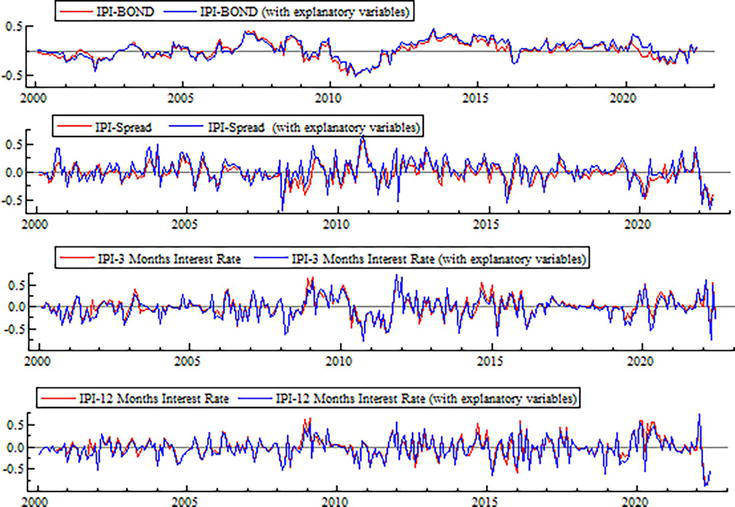
Figure 1 presents the dynamic conditional correlations of the pairs over time. The figures show similar behavior of the correlations regarding the pairs of explanatory variables and without them. Over time, the magnitude of the average correlation between the series is found to be low (the mean magnitude is between −0.02 and 0.04 for all pairs, see Table 5). Specifically, we observed high negative correlations during 2008, which may be an indication of the global financial crisis (GFC). Also, there are high negative correlations during 2015 and turbulences for the next 2-year period. During 2022, there are high negative correlations, which may be due to Russo-Ukranian war.

Figure 1.

The DCCs behavior over time.

Correlation	IPI-Bonds (with expl. Var.)	IPI-Bonds	IPI-Spread (with expl. Var.)	IPI-Spread	IPI-3 Months Interest Rate (with expl. Var.)	IPI-3 Months Interest Rate	IPI-12 Months Interest Rate (with expl. Var.)	IPI-12 Months Interest Rate
Mean	0.0362	0.0059	0.0247	−0.022	−0.0232	−0.001	−0.0358	−0.017
Median	0.0354	0.0161	0.0199	−0.021	−0.0137	−0.002	−0.0365	−0.032
Max.	0.4605	0.4217	0.6603	0.6030	0.7266	0.728	0.7102	0.697
Minimum	−0.5126	−0.5053	−0.6990	−0.617	−0.7723	−0.755	−0.8576	−0.846
Std. Dev.	0.1849	0.1800	0.2061	0.1648	0.2463	0.243	0.2390	0.240
Skewness	−0.3638	−0.3182	−0.3032	−0.153	−0.1207	−0.003	−0.1484	0.025
Kurtosis	2.8889	3.1312	4.2140	4.6230	3.5655	3.812	3.7209	3.966

Table 5.

Descriptive statistics of dynamic correlations.

Notes: In this table, we analyze the descriptive statistics of dynamic correlations from the scalar BEKK and from the scalar BEKK with explanatory variables in the mean equation.

Overall, the relative changes in correlation are larger during volatile periods. The low absolute level of correlations sheds doubts on the magnitude of the dynamic relationship between economic growth and interest rates. While dynamic conditional correlation sheds little light on the scale-dependent characteristics of our series, it is evident that the level of correlation between them is highly dependent on the point in time assessed (see [18] for more details about DCCs’ behavior). This supports the use of dummies in the OLS equation, as well as the application of wavelet coherence for identifying simultaneously the calendar time and scale characteristics of the series.

4.2 The effect of MoUs and pandemic on DCCs behavior

In more depth analysis, we try to examine the effects of the memoranda and pandemic periods on the relationship between economic growth (i.e., IPI), interest rates, spread and bond yield. We use two dummy variables in an OLS equation, which allows us to investigate the dynamic feature of the correlation changes associated with the two periods. We also add a third dummy, which corresponds to a stable period for the Greek economy.

This leads to one important implication from the policymaker’s perspective. A positive statistically significant level of correlation implies that an increase in interest rates will have a positive impact on the real economy and vice versa. When the dummy coefficient is not statistically significant, then the IPI and interest rates are uncorrelated. In parallel, we attempt to detect the sensitivity of the DCC relationship vis-à-vis the type of interest rate, following the technique of Dimitriou and Kenourgios [19]. Thus, we try to investigate the different behaviors between economic growth, interest rates and bonds during crisis periods. We create three dummies, which are equal to unity for the Memoranda, stable and Pandemic periods, respectively and zero otherwise, to the following OLS equation in order to describe the behavior of DCCs over time:

$${\mathit{DCC}}_{\mathit{ij},t}=\mathit{\text{constant}}+\mathit{\text{bDummy}}\_\mathit{MoU}+\mathit{\text{cDummy}}\_\mathit{\text{Stable}}+\mathit{\text{kDummy}}\_\mathit{\text{Pandemic}}+{\epsilon }_{i,t}$$E4

where DCC is the pair-wise Dynamic Conditional Correlations estimated between IPI (i) and the rest variables (j), such that i = IPI, j = the 3-months interest rates (short-term), the 12-months interest rates (long-term), the 10-year Treasury bond, and the spread. Dummy MoU corresponds to the period of Greek Memoranda (01/05/2010 until 01/08/2018).² The Dummy Stable corresponds to a stable period between the two crises that tarnished the Greek economy (01/09/2018–2101/12/2019). Lastly, the Dummy Pandemic corresponds to the period of Pandemic until the end of our sample (01/01/2020–end of our sample).³ As the theoretical model implies, the significance of the estimated coefficients (b, c & k) on the dummy variables indicates structural changes and shifts of the correlation coefficients due to external shocks.

Based on the regression results of Table 6, the evidence shows that in most cases, the dummy coefficients are not statistically significant. Especially, during the memoranda period only the spread displays a positive effect on IPI, indicating its crucial role in economic growth. Obviously, an increase in spreads had a negative impact on the Greek economy. On the other hand, during the stable period, only the bonds have a positive impact on economic growth, at a 10% significance level. This result is contradictory to mainstream theory that by lowering the interest rates the economy is stimulated. However, the success of the longstanding policy of lowering rates in stimulating the economy is in dispute. For example, Federal Reserve economists raised doubts about the wisdom of extremely low-interest rates [20]. Nucera et al. [21] found that negative rates may affect banks negatively, which in turn could harm the economy.

	IPI-Bonds (Mean)	IPI-Bonds	IPI-Spread (Mean)	IPI-Spread	IPI-3-months Interest Rate (Mean)	IPI-3-months Interest Rate	IPI-12-months Interest Rate (Mean)	IPI-12-months Interest Rate
Constant	0.0093	0.0072	0.0189	−0.0255	0.0042	−0.019	−0.0357*	−0.015
Dummy MoU	0.0569	0.0079	−0.0046*	0.0328	−0.0340	−0.013	−0.0039	−0.021
Dummy Stable	0.0905*	0.0570	−0.0055	0.0114	−0.0458	−0.077	−0.0542	−0.033
Dummy Pandemic	0.0028	−0.0688*	−0.101**	−0.085***	0.0840*	0.0528	0.0408	0.0667

Table 6.

Descriptive statistics of dynamic correlations across the three periods.

*

represents 10% statistical significance.

**

represents 5% statistical significance.

***

represents 1% statistical significance.

Notes: Robust standard errors in parenthesis.

The coefficient of the last dummy (pandemic) displays the most statistically significant results, suggesting that during crises, the manipulation of interest rates is needed most. The spread and bond yield have negative impact to IPI, which confirms the mainstream theory, while the 3-months rate follows a different pattern. Perhaps the severity of the crisis leads to a different pattern for short-run interest rates.

Overall, it seems that during the pandemic crisis, the bonds may be useful to stimulate the economy; while during other periods, (crisis or stable) it seems that the correlation between economic growth and interest rates is mostly statistically not significant. This result is interesting because many researchers do not take for granted that interest rate reductions would be positive for the economy.

Finally, following Dimitriou and Kenourgios [19], we provide a sensitivity analysis of the crisis period definition to check the robustness of the results derived from Eq. (4). Firstly, we increase the start date of the two periods in monthly intervals until 3 months onward. In most cases, the estimates of the dummy coefficients in the OLS model indicate similar results. Secondly, we fix the crisis start date of each crisis and the length of each phase is increasing simultaneously in monthly intervals until 3 months onwards. The dummy coefficients change only slightly. To sum up, these results (not reported) indicate that changes due to crisis period definition are rather small and economically insignificant.

4.3 Predictability of models

The ability of a macroeconomic model to predict is crucial, due to its implementation in policymaking and contribution to the stability of the economy. Specifically, a macroeconomic model allows the researcher to investigate the consequences of a policy decision and accordingly adjust its initial specifications. Many policymakers form their decisions according to the forecasting performance of their model. By this way, they can reduce uncertainty and increase credibility when they propose a policy implementation especially related to interest rates and taxes.

Table 7 represents the forecasting of models based on RMSE (a commonly accepted criterion for forecasting performance) that is defined as $\mathit{\text{RMSE}}=\sqrt{{\sum }_{i=1}^2{\left(\mathit{\text{corr}}\left(Y\right)-\mathit{\text{corr}}\left(\widehat{Y}\right)\right)}^2}$. Following Foroni and Marcelino [22] and Doornik et al. [23] we employ 2 steps prediction⁴. The aim of this section is to test the performance of BEKK model and the model with explanatory variables in mean equation. We can observe that the couples IPI-Bond and IPI-3-months interest rate in the model with explanatory variables have 31.88% and 30.28% lower RMSE. Also, the couples IPI-Spread and IPI-12-months interest rates in the model with explanatory variables have 92.45 and 90.3% lower RMSE, respectively. These results indicate the significance of ESI and the general stock exchange index of Athens as explanatories to study microfinance topics.⁵

	RMSE (2-steps Prediction)
Dynamic Correlation	BEKK	BEKK (with explanatory variables)	Change
IPI-Bond	0.470	0.320	−31.88%
IPI-Spread	0.986	0.074	−92.45%
IPI-3-Months Interest Rate	0.57	0.403	−30.28%
IPI-12-Months Interest Rate	0.9595	0.093	−90.30%

Table 7.

Forecasting performance of the models.

4.4 Granger causality analysis

We employ Granger causality test to investigate the causality relationships and its directions between the factors. The methodology is based on the following steps: First, we employ the stationarity tests according to Dickey and Fuller, [24] and Phillips and Perron [25]. Second, we determine the number of lags in VAR model according to lag length criteria and at the second step, we employ the Granger causality test.

The VAR model is defined as

$$\underset{t}{\overset{.}{Y}}={\alpha }_0+\sum _{i=1}^k{\alpha }_{1,i}\underset{t-i}{\overset{.}{Y}}+\sum _{i=1}^k{\beta }_{1,i}{X}_{t-i}+{\epsilon }_{1t}$$E5

$$\underset{t}{\overset{.}{X}}={\gamma }_0+\sum _{i=1}^k{\mathrm{\gamma }}_{1,i}\underset{t-i}{\overset{.}{X}}+\sum _{i=1}^k{\delta }_{1,i}{Y}_{t-i}+{\epsilon }_{2t}$$E6

where X and Y are the endogenous variables, α, β, γ and δ are the parameters, k denotes the number of the lags and ε₁ and ε₂ denote the disturbances.

Regarding the Granger causality, let y_t and x_t be stationary time series, then the general form of this test is:

$$y_t=a_{\mathit{0}}+{\mathit{\Sigma a}}_i{y}_{t-i}+{\mathit{\Sigma \beta }}_j{x}_{t-j}+{ϵ}_t$$E7

$$x_t=a_{\mathit{0}}+{\mathit{\Sigma a}}_i{x}_{t-i}+{\mathit{\Sigma \beta }}_j{y}_{t-j}+{ϵ}_t$$E8

The methodology of Granger determines whether a present variable y_t can be explained by past values of y_t and whether adding lags of another variable x_t improves the explanation. This technique provides useful information about the lead effect of confidence indicators on the macroeconomic variables.

We observe from Table 8 that there are three unidirectional and one bidirectional causality among the variables. Specifically, the results from the causality test show that there is unidirectional causality from IPI to bond, from spread to IPI and from 3-months rate to IPI. We observe bidirectional causality between IPI and 12-months rate.

From	To	Chi-Squared	p-value	Causality
Industrial Production Index	Greece Government Bond 10Y	10.543**	0.032	Yes
Greece Government Bond 10Y	Industrial Production Index	4.179	0.382	No
Industrial Production Index	Spread	5.031	0.284	No
Spread	Industrial Production Index	12.514**	0.0139	Yes
Industrial Production Index	Interest Rate 3-Months	3.419	0.331	No
Interest Rate 3-Months	Industrial Production Index	10.224**	0.017	Yes
Industrial Production Index	Interest Rate 12-Months	12.402**	0.015	Yes
Interest Rate 12-Months	Industrial Production Index	8.811*	0.060	Yes

Table 8.

Granger causality test among our variables.

*

represents 10% statistical significance.

**

represents 5% statistical significance.

4.5 Robustness test using wavelet coherence analysis

We employ this methodology as a robustness check of our main results. Following Torrence and Webster [26], we define the wavelet coherence of two-time series, namely xt and yt, with Wx(τ,s) and Wy(τ,s) wavelet transforms as the absolute value squared of the smoothed cross-wavelet spectrum, normalized by the smoothed wavelet power spectra:

$$R^2\left(\tau ,s\right)=\frac{{\left|S(s^{-1}{W}_{\mathit{xy}}\left(\tau ,s\right)\right|}^2}{S\left(s^{-1}{\left|W_x\left(\tau ,s\right)\right|}^2\right)·S\left(s^{-1}{\left|W_y\left(\tau ,s\right)\right|}^2\right)}$$E9

where S(.) is the smoothing operator and s is the wavelet scale. The R² takes values between zero (no co-movement) and one (perfect co-movement). Monte Carlo methods (3000 simulations) are applied to determine statistical significance, as the distribution of the wavelet coherency is unknown.

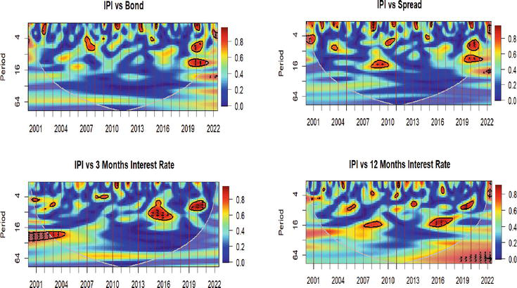
In Figure 2, we present the wavelet coherence analysis between IPI and various interest rates. Red color indicates regions characterized by high interrelation and blue color indicates regions with lower volatility between the two-time series. White transparent area indicates results that are not statistically significant. In this analysis, we focus on short-term period (0–16) and long-term (16–64). Arrows in the figure hold valuable information, as they represent the direction of the relationship of the variables. Specifically, arrows pointing straight up indicate that the first index is leading; arrows straight down indicate that the first index is lagging. Arrows pointing to the right and left show that the two variables are in phase and in antiphase, respectively. If the arrows point to the right and up or to the left and down, it means that the first index is leading. If the arrows point right and down or left and up, it indicates that the first index is lagging.

Figure 2.

Wavelet coherence analysis between IPI and various interest rates. Notes: The white contour designates the 5% significance level estimated from the Monte Carlo simulations using the phase randomized surrogate series. The cone of influence, where edge effects might distort the picture, is shown as a lighter shade. Regions of differing coherency are represented using a heat map, which ranges from blue (low coherency) to red (high coherency). Y-axis measures frequencies or scale and X-axis shows the time period studied (2000–2022). The phase differences between the two series are indicated by arrows. Arrows pointing to the right mean that the variables are in phase (move in the same direction, having cyclical effects on each other). If the arrows point to the right and up, then the first index is leading (the first index causes the second one). If the arrows point down, the first index is lagging. Arrows pointing to the left mean that the variables are out-of-phase (have anti-cyclical effects on each other). If the arrows point to the left and up, the first index is leading and if they point to the left and down, the first index is lagging.

The economic conclusions of the 4.2. subsection seem to remain unaffected. In most cases, the co-movement intensity is low (blue regions). During the short-term period, there are signs of high co-movement (red regions), while during long-term period, low co-movement is observed in almost all cases. One exemption is during the pandemic crisis period where we observe some statistically significant “islands” of higher co-movement in all pairs. To sum up, the results presented in Figure 2 indicate that any existing differences with the DCC outcome are rather small and economically insignificant.

5. Conclusions

This work empirically examined the relationship between Industrial Production Index (used as a proxy of economic growth) and 10-years government bond, 10-years spread, 3-months and 12-months interest rates. By employing several econometric techniques, such as DCCs, Granger causality tests and wavelet coherence analysis, we conclude with an interesting outcome. Since the DCCs behavior over time between the IPI and the other variables is ambiguous, we examined the DCCs behavior during the Memoranda period, Pandemic period and a stable period. The results conclude that in almost all cases, the economic growth remains unaffected by any changes in various interest rates (bond and spread). Only during the pandemic period seems to be a negative relationship for spread and bond in relation to IPI, following the mainstream theory, while the 3-months rate follows a different pattern. Maybe the unique characteristics of the pandemic crisis led to this diverse behavior for the 3-month rate. The robustness test of the wavelet coherence analysis validates the above outcome. The Granger causality test shows a unidirectional causality from IPI to bond, from spread to IPI and from 3-months rate to IPI. Furthermore, there exists a bidirectional causality between IPI and 12-months rate. Another important finding is the better forecasting performance of the extended BEKK model (i.e., with explanatory variables), since it provides 30–90% lower RMSE than the parsimonious model in all cases.

All in all, the finding that prevails in this study is the near complete absence of any statistically significant relationship between economic growth and interest rates, spread and 10-years bond during the Memoranda and stable period for the Greek economy, while there are few cases during the pandemic crisis.

This conclusion adds to recent doubts about the prevailing conduct of monetary policy and common theoretical models (e.g., lowering interest rates may have no effect, when trying to stimulate the economy). These results provide crucial implications for policymakers and highlight the need for some form of policy coordination among central banks.

Conflict of interest

The views and opinions expressed in this article are those of the authors and do not necessarily reflect those of the Hellenic Fiscal Council. Any errors are ours.

References

1.Lee KS, Werner RA. Are lower interest rates really associated with higher growth? New empirical evidence on the interest rate thesis from 19 countries. International Journal of Finance and Economics. 2022;28:3960-3975. DOI: 10.1002/ijfe.2630
2.Harvey CR. Forecasts of economic growth from the bond and stock markets. Financial Analysts Journal. 1989;45(5):38-45
3.Ferreira E, Martínez Serna MI, Navarro E, Rubio G. Economic sentiment and yield spreads in Europe. European Financial Management. 2008;14(2):206-221
4.Ang A, Piazzesi M, Wei M. What does the yield curve tell us about GDP growth? Journal of Econometrics. 2006;131(1–2):359-403
5.Dotsey M. The predictive content of the interest rate term spread for future economic growth. FRB Richmond Economic Quarterly. 1998;84(3):31-51
6.Liu E, Mian A, Sufi A. Low interest rates, market power, and productivity growth. Econometrica. 2022;90(1):193-221
7.Shaukat B, Zhu Q, Khan MI. Real interest rate and economic growth: A statistical exploration for transitory economies. Physica A: Statistical Mechanics and its Applications. 2019;534:122193
8.Udoka CO, Anyingang RA. The effect of interest rate fluctuation on the economic growth of Nigeria, 1970–2010. International Journal of Business and Social Science. 2012;3(20):295-302
9.Del Negro M, Giannone D, Giannoni MP, Tambalotti A. Global trends in interest rates. Journal of International Economics. 2019;118:248-262
10.Blanchard O. Public debt and low interest rates. American Economic Review. 2019;109(4):1197-1229
11.Albu AC, Albu LL. Public debt and economic growth in euro area countries. A wavelet approach. Technological and Economic Development of Economy. 2021;27(3):602-625
12.Hayat MA, Ghulam H, Batool M, Naeem MZ, Ejaz A, Spulbar C, et al. Investigating the causal linkages among inflation, interest rate, and economic growth in Pakistan under the influence of COVID-19 pandemic: A wavelet transformation approach. Journal of Risk and Financial Management. 2021;14(6):277
13.Crowley PM, Hudgins D. Monetary policy objectives and economic outcomes: What can we learn from a wavelet-based optimal control approach? The Manchester School. 2022;90(2):144-170
14.Odo L, Bosnjak M. A comparative analysis of the monetary policy transmission channels in the US: A wavelet-based approach. Applied Economics. 2021;53(38):4448-4463
15.Armelius H, Hull I, Köhler HS. The timing of uncertainty shocks in a small open economy. Economics Letters. 2017;155:31-34
16.Bilgili F. Business cycle co-movements between renewables consumption and industrial production: A continuous wavelet coherence approach. Renewable and Sustainable Energy Reviews. 2015;52:325-332
18.Dimitriou D, Kenourgios D, Simos T. Are there any other safe haven assets? Evidence for “exotic” and alternative assets. International Review of Economics & Finance. 2020;69:614-628
19.Dimitriou D, Kenourgios D. Financial crises and dynamic linkages among international currencies. Journal of International Financial Markets, Institutions and Money. 2013;26:319-332
20.Kliesen K. Low interest rates have benefits… and costs. The Regional Economist. 2010;15:6-7
21.Nucera F, Lucas A, Schaumburg J, Schwaab B. Do negative interest rates make banks less safe? Economics Letters. 2017;159:112-115
22.Foroni C, Marcellino M. A comparison of mixed frequency approaches for nowcasting euro area macroeconomic aggregates. International Journal of Forecasting. 2014;30(3):554-568
23.Doornik JA, Castle JL, Hendry DF. Short-term forecasting of the coronavirus pandemic. International Journal of Forecasting. 2022;38(2):453-466
24.Dickey DA, Fuller WA. Likelihood ratio statistics for autoregressive time series with a unit root. Econometrica: Journal of the Econometric Society. 1981;49:1057-1072
25.Phillips PC, Perron P. Testing for a unit root in time series regression. Biometrika. 1988;75(2):335-346
26.Torrence C, Webster PJ. The annual cycle of persistence in the El Nño/southern oscillation. Quarterly Journal of the Royal Meteorological Society. 1998;124(550):1985-2004
Notes
See prior literature such as Armelius et al. [15], and Bilgili [16].
On May 2, 2010, the Eurogroup agreed to provide bilateral loans pooled by the European Commission (Greek Loan Facility – GLF) for a total amount of €80 billion to be released over the period May 2010 to June 2013. The third and final financial assistance program to Greece ended on August 20. As of this date, the country is no longer reliant on ongoing external rescue loans for the first time since 2010. Greece now enters post-program monitoring.
The World Health Organization declared the COVID-19 outbreak a Public Health Emergency of International Concern on January 30, 2020, and a pandemic on March 11, 2020.
Foroni and Marcelino [22] have employed two-steps prediction with monthly data and Doornik et al. [23] employed one, two, four and seven steps on monthly data.
However, we cannot rule out the possibility that other forecasting methods could show that economic confidence indices do indeed have improved explanatory power, if any such methods can be found.
Written By
Dimitrios Dimitriou, Alexandros Tsioutsios, Theodore Simos and Dimitris Kenourgios
Submitted: 25 January 2024Reviewed: 26 January 2024Published: 28 February 2024