Statistical Methods Applied in Modeling Corrosion Depth Measurement on Three Different Shape Memory Alloys

Abstract

This chapter presents a study focused on the corrosion behavior of three distinct shape memory alloys (CuAlNi and two types of NiTi alloys) in varied marine environments—air, tide, and seawater. The research documents corrosion damage after 6, 12, and 18 months, utilizing focused ion beam. Scanning electron microscopy and energy dispersive X-ray analyses were employed to detect the chemical alterations. This study includes both deterministic and stochastic frameworks for modeling corrosion processes. Employing a range of statistical techniques, including linear and multivariate regression, principal component analysis, and correlation analysis (linking corrosion depth with oxygen presence), the research provides an in-depth understanding of corrosion dynamics. The study explores fitting standard two-parameter and advanced multi-parameter distributions to the observed data. The dual treatment of corrosion parameters via linear and non-linear models enhances the robustness and applicability of our findings, offering more precise and effective corrosion management in marine engineering applications.

1. Introduction

In the past century, research in smart materials, including alloys, polymers, ceramics, composites, and hybrids, has been extensive, with notable achievements in shape memory alloys (SMA). The phenomenon was first identified in 1932 with gold-cadmium alloys by a Swedish physicist, marking the beginning of SMA research [1]. The shape memory effect (SME) was later observed in copper-zinc and copper-tin alloys in 1938 by Greninger and Mooradian [2], leading to the discovery of the NiTi alloy by William Buehler in 1959, paving the way for nitinol’s commercialization from 1962 [3, 4]. SMAs have since found diverse applications in medicine, aerospace, and more due to their unique thermo-mechanical properties, including SME, superelasticity, and high damping capacity [5, 6]. Research continues to enhance SMAs, particularly focusing on NiTi, Cu, and Fe-based systems to improve their properties for broader applications. NiTi alloys are especially valued for their biocompatibility and thermal stability, with efforts to extend their usability beyond 80°C through new compositions [7]. Cu-based SMAs, notably CuAlNi alloys, are distinguished by their thermal stability and cost-effectiveness, despite challenges with ductility and production [5, 7, 8]. Innovations in alloying and processing aim to overcome these challenges, enhancing the functionality and application scope of SMAs [9, 10].

1.1 Shape memory alloys in marine environments

While SMAs are less commonly used in marine and maritime sectors compared to medicine and transportation, their potential applications range from deep-sea tube connections to surface-level technologies, thanks to their superelastic properties. SMAs offer solutions for tension-leg platforms, subsea equipment thermostats, and thermal energy transfer in undersea power plants [11]. Their suitability depends on mechanical, chemical, physical, and thermo-mechanical traits, particularly corrosion resistance. Austenitic structures in SMAs show higher corrosion resistance than martensitic structures, attributed to the hyperplastic behavior of their polycrystalline structure [12]. However, porous NiTi SMAs face high corrosion rates due to their surface characteristics, while stress corrosion leads to cracking in NiTi alloys [13]. Research on CuZnNi alloys indicates improved corrosion resistance with increased nickel or zinc content [13]. Adding aluminum to Cu-based alloys enhances corrosion resistance through alumina layer formation, with nickel playing a crucial role in the passivation of Cu-Ni alloys [5]. Studies on CuAlNi alloys in varying chloride ion concentrations show that higher concentrations increase corrosion, evidenced by increased corrosion current density and decreased polarization resistance [8].

1.2 Corrosion rate of metal structures in marine environments

Corrosion significantly accelerates metal degradation under environmental influences. Past research developed models for pitting and general corrosion based on corrosion depth, rate, and causative conditions. Traditionally, new materials were tested in labs or briefly in natural settings, lacking long-term material observation. These models predict corrosion likelihood by identifying key factors and mechanisms, supported by statistical models that calculate corrosion rates’ average and standard deviation in real-world applications, notably in ship structural materials [14, 15, 16, 17, 18, 19].

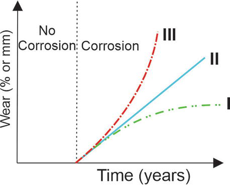
Figure 1 showcases existing corrosion models, reflecting research findings and time-based corrosion progression analysis. Initial investigations of the corrosion process indicated an unstable and time-dependent process that can be described by a linear dependence (curve II). However, recent research has shown that non-linear models more accurately describe the corrosion process (curves II and III). If corrosion increases and accelerates with time (line III), the corrosion process takes place in dynamically loaded structures that are immersed in seawater. Contrary to the above, if the corrosion rate increases at the beginning of the process but decreases slightly as the corrosion process progresses in time, (line I), the corrosion process takes place in an insoluble environment, that is, atmospheric conditions, when the steel is significantly covered by a corrosion layer which prevents further exposure of the materials to the corrosive environment. Corrosion is prevented by surface coatings but initiates upon their deterioration, as depicted by curves I and III in Figure 1. While many researchers view corrosion as a time-dependent and unstable process, typically linearly modeled (curve II in Figure 1), experimental studies suggest that non-linear models better capture certain environmental condition corrosion processes.

Figure 1.

Overview of corrosion rate model.

The corrosion pattern over time for submerged structures tends to be concave (curve III), reflecting continuous exposure to corrosive elements, especially under dynamic strain. Conversely, corrosion, that initially accelerates then slows, is illustrated by curve I, typical for non-submerged structures protected by a corrosive layer.

Investigations into vessel corrosion highlight the acceleration due to atmospheric exposure, vessel operation, and seawater’s biological, chemical, and physical factors. The interaction among marine environment factors like dissolved oxygen, pH, temperature, water movement, salinity, sulfate-reducing bacteria, galvanic coupling, and marine growths significantly influences corrosion rate and mechanism. Thus, understanding these interrelationships is crucial for predicting metal structure corrosion in marine applications.

2. Materials and methods

This study explores the impact of three distinct environmental conditions on CuAlNi and two NiTi alloys’ corrosion processes. Two environments are static—the atmosphere and the sea—while the third, the tidal zone, is dynamic, characterized by cyclic wet and dry conditions due to tidal changes. Over 18 months, the experiment evaluated the corrosion behavior and chemical composition changes, including oxygen content, on the surface of CuAlNi, NiTi1, and NiTi2 alloy samples. Corrosion depth and surface chemical composition were assessed using two specific measurement techniques to understand the alloys’ response to these environments after 6, 12, and 18 months of exposure.

2.1 Materials

The NiTi alloys were produced using vacuum and continuous casting methods, with materials supplied by Zlatarna Celje d.o.o., Slovenia. This research produced two variants of NiTi alloys: one through classical casting (NiTi1) at a specific temperature and pressure, and another (NiTi2) through a combination of vacuum remelting and continuous casting, as detailed in prior studies [20, 21]. Samples were prepared for testing with specific shapes to facilitate attachment during experiments. The preparation process involved several steps: cutting, mounting, grinding, polishing, cleaning, and chemical etching to reveal the microstructures for analysis under a light microscope, highlighting their dendritic patterns, influenced by the casting method and cooling rates [22].

CuAlNi shape memory alloy (SMA) bars were produced using a laboratory-scale vertical continuous casting device connected to a vacuum induction melting (VIM) furnace, allowing for customizable withdrawal speeds to suit various research approaches [20]. The manufacturing process involved high-purity metals: copper, aluminum, and nickel, all sourced from Zlatarna Celje d.o.o., Slovenia. These bars were then precisely shaped into test samples through electro-erosion, with dimensions tailored for corrosion experiments. Post-manufacture, the samples were meticulously prepared through grinding, polishing, and etching to facilitate initial microstructural inspections essential for corrosion testing. This preparatory phase was crucial for ensuring accurate microstructure analysis and microhardness measurements, which were complemented by chemical composition analysis using advanced spectroscopy and X-ray fluorescence techniques [22]. The detailed approach to sample preparation and analysis underscores the rigorous methodology applied in studying the corrosion resistance and properties of CuAlNi SMAs, with findings documented in specified figures and tables for comprehensive understanding.

Environmental exposure tests placed samples in atmospheric, tidal, and submerged marine conditions to observe corrosion effects. This methodology aligns with a conceptual research model outlined in a previous article [23]. Metallographic and microstructural observations were performed to assess corrosion [22, 24], complemented by chemical composition analysis using inductively coupled plasma analyses (ICP analyses) and fluorescent X-ray analyses (XRF analyses) on surfaces exposed to different environmental conditions, presenting the findings in Table 1 [22].

Sample	%Cu		%Al		%Ni		%Ti		%Fe
	ICP	XRF	ICP	XRF	ICP	XRF	ICP	XRF	ICP	XRF
CuAlNi	Base	Base	12	9.4–9.6	3.9	4.4			0.03
NiTi1					55.4	55.2–55.5	44.6	44.4–44.8	/	/
NiTi2					62.6	62.5–62.6	35.9	35.9	1.4	1.4

Table 1.

Chemical composition of the CuAlNi, NiTi1, and NiTi2 samples.

The study involved examining CuAlNi alloy samples across three distinct environments. At the first location, three samples were placed near the sea, elevated three meters above the surface, to study atmospheric and marine environmental impacts. The second group was positioned at the sea surface, subject to varying atmospheric and marine conditions due to tidal movements and wave action in the splash zone. The third group was submerged three meters deep in the sea near the coast.

The analysis was twofold: measuring corrosion depth using focused ion beam (FIB) characterization after 6 and 12 months and employing a linear corrosion model for distribution function optimization. Additionally, semi-quantitative snalysis provided insights into how different environments affected the alloy’s chemical surface composition through principal component analysis.

Material characterization employed FIB/SEM for physical processing and sub-surface imaging. Chemical composition analysis utilized high-resolution SEM equipped with an EDX detector, enabling the detailed examination of corrosion effects and elemental surface content on the CuAlNi samples under various magnifications.

2.2 Methods

The research investigates the corrosion rate estimation for CuAlNi samples across three different environments using a model referenced from Qin and Cui [25]. This model articulates corrosion wear as a function of time, represented by

$$d\left(t\right)=c_1{\left(t-T_{cl}\right)}^{c_2},$$E1

where $d\left(\text{t}\right)$ is the corrosion depth in nanometers, $t$ is the time elapsed since exposure, $T_{cl}$ is the coating life, and $c_1$ and $c_2$ are constants [26]. The model challenges the assumption of a constant corrosion rate, suggesting that a non-linear approach may be more accurate [27, 28]. This study particularly validated the expression with $c_2=1$ by Paik, Kim, and Lee [14], assuming immediate corrosion initiation $T_{cl}=0$ [17] due to the absence of anti-corrosion coating on the samples. The average corrosion depths at various times provided data to approximate $c_1$, reflecting the CuAlNi alloy’s response to seawater exposure.

Predictive tools are vital for analyzing the behavior of physical phenomena, necessitating the development of models to draw general conclusions from empirical data. This involves selecting known variables to predict based on other explanatory variables. Linear regression, a foundational predictive modeling approach, starts with defining independent variables and identifying dependent variables to model responses. It progresses through estimating parameters to minimize prediction errors, concluding with tests to confirm the model’s accuracy. Linear regression splits into simple regression, with one independent variable, and multivariate regression, incorporating multiple variables [29]. The linear regression formula, where Y is the dependent variable and X represents the independent variables [30], includes an intercept (${\beta }_0$) and coefficients (${\beta }_0,{\beta }_1,{\beta }_2,\dots ,{\beta }_N$) that must be estimated to best describe Y’s linear relationship with X, as it is shown in Eq. (2).

$$Y={\beta }_0+{\beta }_1{x}_1+{\beta }_2{x}_2+\dots +{\beta }_N{x}_N.$$E2

Once established, this model predicts Y’s value for given X values.

Cluster analysis (CA) and principal component analysis (PCA) are prominent multivariate techniques utilized for the organization and interpretation of complex and diverse experimental datasets, identifying patterns and relationships within [31, 32, 33, 34]. These methods are praised for their efficiency in classifying extensive data from varied sources and streamlining information by removing redundancies. Statistical analyses were conducted using Statistics 13.5.017 software (StatSoft Inc., Tulsa, OK, USA), while Origin 6.1 software facilitated the experimental data analysis. Specifically, PCA applied to a matrix—corrosion parameters from EDX analyses as variables against alloy sample spectra—underwent standardization to equalize all parameter significance before analysis.

2.3 Data collection

The research involved examining alloy samples across three sites during 2018 and 2019 to assess seawater’s impact on corrosion, particularly in the Bay of Kotor, based on extensive pre-research observations. Observational data highlighted that both sea and atmospheric average temperatures remained below 20°C, with the sea consistently warmer than the air, showing minimal temperature fluctuations in the sea compared to air [35, 36]. The study noted stable seawater conditions up to 5 meters deep, with minor variations in temperature, conductivity, and salinity, which, along with the higher sea temperatures and the effects of seasonal freshwater inflow reducing salinity and conductivity from September to May, suggested that corrosion rates in the marine environment could be more rapid than in atmospheric conditions due to these factors.

3. Results

Table 2 presents fundamental descriptive statistics, including the mean, standard deviation (StD), minimum, first quartile (Q1), median, third quartile (Q3), and maximum, derived from the empirical database for CuAlNi samples. It outlines the number of data points (N), along with statistical metrics for both the oxygen percentage (O) and corrosion depth (d, measured in nm) across various environmental conditions. Similarly, Tables 3 and 4 follow the same format but focus on descriptive statistics for the empirical datasets concerning corrosive processes in NiTi1 and NiTi2 alloys.

		N	Mean	StD	Min	Q1	Median	Q3	Max
Air	O	47	30.61	12.44	5.1	22.65	28.38	38.32	63.46
	d	47	506.5	321.57	116.67	187.5	575	758.38	1200
Tide	O	49	35.22	14.8	3.68	26.84	38.32	47.92	57.35
	d	49	1418.1	674.34	545.83	829.17	1250	1995	3050
Sea	O	57	38.67	12.46	0.00	32.51	38.38	47.6	56.99
	d	57	1570.1	661.62	482.14	864.58	1770	2035	3170

Table 2.

The statistical summary of the input data on the CuAlNi alloy.

		N	Mean	StD	Min	Q1	Median	Q3	Max
Air	O	31	11.41	10.15	0.00	2.02	8.28	19.34	30.00
	d	31	43.36	8.84	30.00	37.50	40.00	50.00	58.33
Tide	O	41	29.90	8.68	9.14	24.77	28.57	35.61	48.41
	d	41	38.78	10.86	22.50	30.00	37.50	45.83	66.67
Sea	O	49	26.67	13.16	0.00	15.04	29.82	37.63	52.48
	d	49	281.3	158.5	41.7	168.8	308.3	414.6	575.0

Table 3.

The statistical summary of the input data on the NiTi1 alloy.

		N	Mean	StD	Min	Q1	Median	Q3	Max
Air	O	84	19.73	7.812	4.110	15.60	20.63	23.80	38.97
	d	84	54.89	15.44	29.17	45.21	55.00	62.50	95.83
Tide	O	71	41.05	26.80	5.00	16.92	38.26	56.80	141.67
	d	71	156.5	147.1	37.5	47.5	72.5	258.3	708.3
Sea	O	64	57.52	41.28	0.00	30.86	42.09	72.08	171.7
	d	64	286.2	202.7	70.8	139.4	215.8	376.0	858.3

Table 4.

The statistical summary of the input data on the NiTi2 alloy.

In practical experiments, physical quantities typically exhibit interdependencies where changes in one variable affect one or more others. Constructing models that accurately depict these causal relationships between variables is crucial for predicting future values or estimating dependent quantities. Various types of correlations exist in statistical analysis, all aiming to capture the causal changes of one variable concerning others, considering both the tendency and intensity of these changes. This chapter employs Pearson’s correlation coefficient [37], a widely used correlation metric.

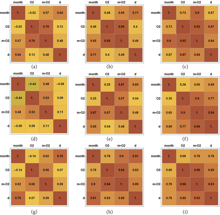
Figure 2 illustrates the correlation analysis results, focusing on the corrosion depth as the dependent variable and the percentage of oxygen, elapsed time since the experiment’s onset, and the concurrent influence of oxygen and exposure time as independent variables. Correlation matrices are presented for each alloy across the three seawater environments. The columns show the behavior of each alloy, while the rows show the behavior in the observed environment, that is, Figure 2a–c are related to the alloy’s behavior in air, Figure 2d–f are related to the alloy’s behavior in the tide, while Figure 2g–i depict alloy’s behavior in the sea.

Figure 2.

Pearson’s correlation: (a) CuAlNi in the air, (b) NiTi1 in the air, (c) NiTi2 in the air, (d) CuAlNi in the tide, (e) NiTi1 in the tide, (f) NiTi2 in the tide, (g) CuAlNi in the sea, (h) NiTi1 in the sea, and (i) NiTi2 in the sea.

Pearson’s correlation coefficient ranges between −1 and 1, with negative values indicating a negative correlation and positive values indicating a positive correlation between the observed variables. Across all three environmental types and for both alloys, only positive correlation effects are observed in Figure 3a–f. Specifically, an increase in one variable corresponds to an increase in the other. The degree of correlation varies from high to low, or it can be non-existent, characterized by coefficient values between ±0.50 and ± 1, ± 0.30 and ± 0.49, and below ±0.29, respectively. Correlation matrices in Figure 2 visually represent these correlation degrees, with the intensity of brown color indicating the strength of correlation. Each observed alloy and marine environment type is represented by a correlation matrix, illustrating the degree of correlation between variables and the corresponding Pearson correlation coefficient values. As anticipated, all alloys demonstrate a tendency for increased corrosion depth across all observed marine environments (air, tide, and sea) concerning prolonged exposure duration and oxygen percentage.

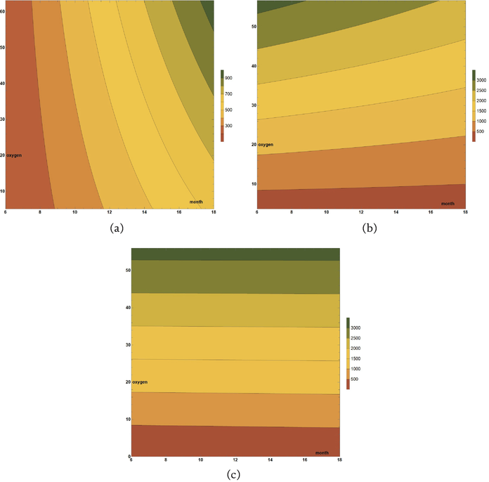
Figure 3.

CuAlNi linear models’ visualization: (a) air, (b) tide, and (c) sea.

To model the corrosive behavior of CuAlNi alloy in three different marine environments, linear regression was applied to the corrosion depth as a dependent variable in Eq. (2). In this way, three different models were formed for the depth of corrosion denoted by ${\text{d}}_{CuAlNi}^{air},{\text{d}}_{CuAlNi,}^{tide}\text{and}{\text{d}}_{CuAlNi}^{sea}$ and shown in Eqs. (3)–(5).

$${\text{d}}_{CuAlNi}^{air}=33.15\ast \text{month}-2.58\ast {\text{O}}_2+0.45\ast \text{month}\ast {\text{O}}_2,$$E3

$${\text{d}}_{CuAlNi}^{tide}=70.68\ast \text{month}+28.99\ast {\text{O}}_2-1.24\ast \text{month}\ast {\text{O}}_2,$$E4

$${\text{d}}_{CuAlNi}^{sea}=105.93\ast \text{month}+9.36\ast {\text{O}}_2-0.057\ast \text{month}\ast {\text{O}}_2.$$E5

Figure 3 shows visual representations of the formed models given by Eqs. (3)–(5) for CuAlNi alloy. The x-axis shows the independent variable month, which represents the time the alloy was exposed to the environment, while the y-axis shows another independent variable, that is the percentage of oxygen. Corrosion depth, as a dependent variable, is shown on the scale in the legend, with different colors depending on the interval to which the resulting corrosion depth belongs, calculated through the formed linear model.

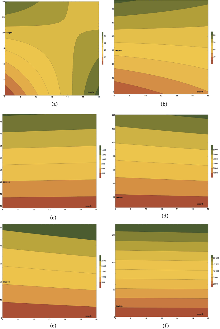
Similar to the case of the CuAlNi alloy, and in the case of the NiTi1 and NiTi2 alloys, linear regression was applied to determine how the depth of corrosion changes depending on the influence of independent variables, which in this chapter are the month, the percentage of oxygen, and the mutual interaction of the elapsed time of the alloys exposure to the influence of the environment together with the percentage of oxygen (month*O₂). Three models were formed for each of the NiTi alloys, one for each observed environment (air, tide, and sea). In this way, a total of six models were formed, which are shown by the expressions given in Eqs. (6)–(11).

$${\text{d}}_{NiTi1}^{air}=3.43\ast \text{month}+2.28\ast {\text{O}}_2-0.16\ast \text{month}\ast {\text{O}}_2,$$E6

$${\text{d}}_{NiTi1}^{tide}=4.01\ast \text{month}+0.71\ast {\text{O}}_2-0.08\ast \text{month}\ast {\text{O}}_2,$$E7

$${\text{d}}_{NiTi1}^{sea}=12.09\ast \text{month}-0.21\ast {\text{O}}_2+0.35\ast \text{month}\ast {\text{O}}_2,$$E8

$${\text{d}}_{NiTi2}^{air}=1.86\ast \text{month}+2.57\ast {\text{O}}_2-0.07\ast \text{month}\ast {\text{O}}_2,$$E9

$${\text{d}}_{NiTi2}^{tide}=2.26\ast \text{month}-1.32\ast {\text{O}}_2+0.33\ast \text{month}\ast {\text{O}}_2,$$E10

$${\text{d}}_{NiTi2}^{sea}=11.29\ast \text{month}-0.47\ast {\text{O}}_2+0.21\ast \text{month}\ast {\text{O}}_2.$$E11

The formed six models shown through Eqs. (6)–(11) are visually presented in Figure 4. Figure 4 clearly shows the similarities and differences in the behavior of NiTi1 and NiTi2 alloys in three different environments.

Figure 4.

Linear models visualization: (a) NiTi1 air, (b) NiTi2 air, (c) NiTi1 tide, (d) NiTi2 tide, (e) NiTi1 sea, and (f) NiTi2 sea.

The chapter emphasizes that many stochastic factors influence corrosion, suggesting that the $c_1$ coefficient is better modeled as a continuous random variable rather than a fixed value. It introduces a probabilistic method to estimate the cumulative distribution function (CDF) of the corrosion rate ($c_1$), employing statistical analysis to understand $c_1{}^{’}$s variability. Assuming the linear corrosion model $\text{d}\left(\text{t}\right)={\text{c}}_1\text{t}$ holds, it allows for empirical determination of $c_1{}^{’}$s CDF, facilitating the fitting of two-parameter distributions to these empirical data points. This approach leads to identifying the most appropriate two-parameter distributions for describing corrosion rates across different environmental conditions: air, tides, and sea, analyzing 27 common two-parameter distributions [38] for each environment.

To identify the most accurate two-parameter or multi-parameter distributions for empirical corrosion rate data ($c_1$), statistical analysis validated by the Kolmogorov–Smirnov test was performed. This test, advantageous for its non-parametric and distribution-free nature, assesses if empirical data align with a continuous theoretical distribution through null and alternative hypotheses. It evaluates the fit of a probability function to the measured data by comparing the p-value against a critical value at a predetermined significance level, determining the quality of the fitted distribution. The chapter details these processes, including significance levels and critical values used.

When the test statistic surpasses the critical value for a chosen significance level α, the hypothesis about the distribution’s form is rejected. The p-value, derived from the test statistic, signifies the lowest significance level at which the null hypothesis is upheld. If the p-value falls below the critical threshold, the null hypothesis is dismissed, indicating that the theoretical distribution fails to accurately represent the empirical data at the chosen level of significance. This analysis involves comparing calculated test statistics against critical values to assess the fit between theoretical and empirical distributions. The study also employs Probability density functions (PDF) and cumulative distribution functions (CDF) to fit theoretical distributions to corrosion rate data from various environments, utilizing maximum likelihood estimation for parameter determination.

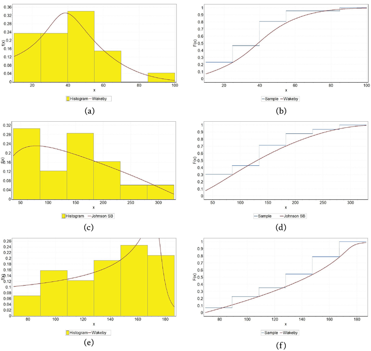
Figures 5–7 show the PDF and CDF for the theoretical distributions that best fit the empirical data for each alloy. The first column of the table shows graphs for the PDF distributions that proved to be the most adequate for describing the corrosive behavior of alloys in the observed marine environment, while the second column of these tables shows the graph for the corresponding CDF of the best theoretical distributions.

Figure 5.

Fitting theoretical distributions to coefficient c₁ for CuAlNi alloy: (a) PDF for air, (b) CDF for air, (c) PDF for tide, (d) CDF for tide, (e) PDF for sea, and (f) CDF for sea.

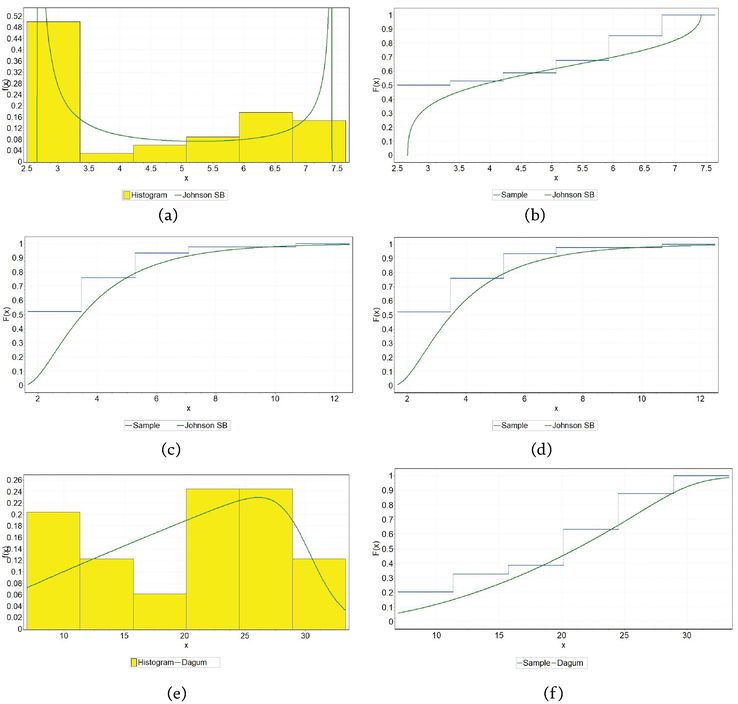
Figure 6.

Fitting theoretical distributions to coefficient c₁ for NiTi1 alloy: (a) PDF for air, (b) CDF for air, (c) PDF for tide, (d) CDF for tide, (e) PDF for sea, (f) CDF for sea.

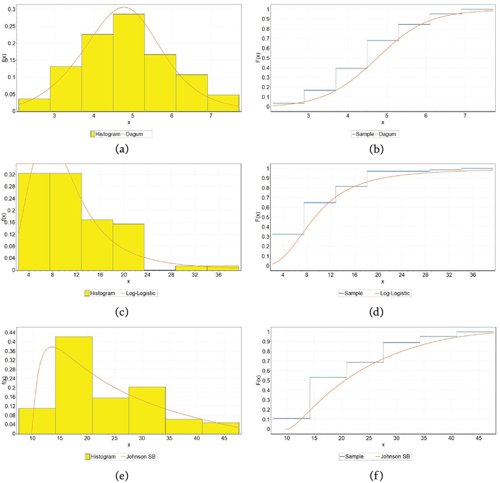
Figure 7.

Fitting theoretical distributions to coefficient c₁ for NiTi2 alloy: (a) PDF for air, (b) CDF for air, (c) PDF for tide, (d) CDF for tide, (e) PDF for sea, (f) CDF for sea.

Table 5 contains distribution data for three alloys (CuAlNi, NiTi1, and NiTi2) in three different environments (air, tide, and sea). Each cell in the table specifies a type of distribution along with its parameters, which are characteristic of how corrosion depth behaves under each condition for the respective alloy. These distributions are used to model the corrosion data, and the parameters provided represent shape, scale, and location parameters that are essential in describing the specific distribution’s characteristics.

	CuAlNi	NiTi1	NiTi2
Air	Wak(136.3,5.4,22.7,-0.2,0)	JSB(0.3,0.3,4.8,2.7)	Dag(0.53,9.4,5.29)
Tide	JSB(0.5,0.9362.06,0.3)	JSB(3,1.2,27.7,1.3)	LL(2.76,9.35)
Sea	Wak(190.3,1.9,1.6,0.36,69)	Dag(0.09,20.8,30.4)	JSB(0.96,0.8,45.7,9.74)

Table 5.

Parameters of the best-fitted theoretical distributions.

Among the 27 different continuous theoretical distributions that were considered, the two-parameter log-logistic distribution (LL) in the case of NiTi2 alloy under the influence of the tide, the three-parameter Dagum distribution (Dag) in the case of NiTi1 alloy under the influence of the sea and NiTi2 alloy under the influence of air, proved to be the best, and multi-parameter Johnson SB (JSB) and Wakeby (Wak) in the case of the remaining alloys considered in other marine environments.

The determination and ranking of the optimal theoretical distributions were directed through the outcomes of the Kolmogorov-Smirnov (KS) test. The capacity to rank these distributions stemmed from the computed KS test statistic values. Smaller KS statistic values represented a closer alignment of the theoretical distributions with the empirical data, enhancing the distribution’s rank accordingly.

For assessing significance, standard levels such as 0.01, 0.02, 0.05, 0.1, and 0.5 were employed. Each level of significance, α, had an associated critical value identified. The hypothesis of data adhering to a specified distribution (H0) would be dismissed if the KS test’s computed statistic surpassed the critical value at the given α. The KS test generates a p-value based on its statistic, representing the minimal significance level at which the null hypothesis, suggesting the data conforms to the theoretical distribution, remains unchallenged. Essentially, if the p-value is notably low, it implies that the data’s compatibility with the chosen distribution is unlikely. For all analyzed distributions, the KS statistics did not exceed the critical thresholds for the selected levels of significance, nor did they surpass the corresponding p-values, indicating no basis to reject H0.

The previous studies explored the corrosion dynamics of NiTi [39] and CuAlNi [38] alloys exposed to varied marine environments for 6–12 months, employing energy dispersive X-ray (EDX) analysis and multivariate statistical methods like principal component analysis (PCA) and cluster analysis (CA) for in-depth interpretation. Our analysis, aligned with other studies, demonstrates that PCA coupled with EDX results can effectively discern various environmental influences on metal degradation.

For NiTi alloys, the EDX analysis unveiled notable disparities in chemical compositions across different environmental conditions, illustrating a pronounced formation of inorganic salts, predominantly sodium, calcium, and magnesium, indicative of corrosion. The multivariate analysis, through PCA and CA, elucidated distinct corrosion behaviors under diverse environmental exposures, with sea conditions notably accelerating the corrosion process, manifesting in heterogeneous surface conditions.

PC1 versus PC2 score plot and cluster analysis [39] further validated the distinct environmental effects on alloy corrosion. The cluster analysis notably grouped the examined environments into two main clusters, with further division into subclusters, indicating the nuanced differences in corrosion behavior among the environments.

Similarly, the corrosion behavior of CuAlNi alloys was scrutinized, revealing consistent patterns under varying conditions. PCA depicted a unique corrosion pattern for CuAlNi alloys exposed to sea conditions, differentiating them from those subjected to air and flood tides, with distinct principal component values underscoring this variation. Over time, this analysis highlighted a stable trend of corrosion behavior in sea and air environments, while flood tides exhibited a dynamic influence on the corrosion mechanism of CuAlNi alloys.

The PCA results highlight distinct trends in corrosion behavior, revealing significant differences among environments. Specifically, PCA identified differences in corrosion behavior between exposure to flood tides, air, and seawater. Samples exposed to seawater exhibited positive PC2 values, while those exposed to air showed positive PC1 values and negative PC2 values. Flood tide exposure resulted in negative PC1 and PC2 values, distinguishing it from air-exposed samples.

Our study [38] explored how exposure duration affects corrosion. The correlation between PC1 and PC2 after 12 months of exposure indicates changes in corrosion behavior over time. Notably, while the separation between air-exposed samples remained consistent, samples exposed to seawater and flood tides showed less differentiation after 12 months, suggesting a shift in corrosion mechanisms over time.

We further analyzed EDX data using PCA for each environment at both 6- and 12-month intervals. Results revealed distinct corrosion behaviors influenced by the environment and exposure duration. Seawater and flood tides exhibited similar effects on corrosion behavior, with a clear separation between samples at both time points. In contrast, the corrosive effects of air showed less variation between 6 and 12 months, indicating slower corrosion compared to seawater and flood tides.

4. Discussion

Based on the descriptive statistics, we can draw comparisons across the three alloys (CuAlNi, NiTi1, and NiTi2) in various environments (air, tide, and sea).

CuAlNi exhibits increasing mean corrosion depth and oxygen percentage from air to sea environments, indicating heightened corrosion in more aggressive environments. NiTi1 shows a distinct pattern with lower oxygen percentages and corrosion depths in air, with a significant increase in sea environments, suggesting sensitivity to environmental aggressiveness. NiTi2 demonstrates variability in corrosion behavior with the highest oxygen percentage in the sea, indicating a pronounced environmental impact, especially in saline conditions.

Under air influence, NiTi1 shows significantly lower oxygen percentages and corrosion depths compared to CuAlNi and NiTi2, indicating its superior resistance to air-induced corrosion. NiTi2 and CuAlNi have higher means in both metrics, with NiTi2 showing greater variability in oxygen levels. NiTi2 exhibits a dramatically higher range and mean in oxygen percentages and corrosion depths under tide influence, suggesting its higher sensitivity to tidal conditions. CuAlNi and NiTi1 show less variability, with CuAlNi experiencing the most severe corrosion depth. Across the sea environment, NiTi2 again displays the highest oxygen percentages, indicative of severe corrosion. CuAlNi follows with significant corrosion depth, while NiTi1 shows a balance between resistance and susceptibility to sea conditions.

The Pearson correlation analysis investigates the interrelationships among various variables, with a specific focus on how the depth of corrosion (d) correlates with other factors including the elapsed time since the experiment’s onset (month), the percentage of oxygen (O₂), and the interaction between time and oxygen percentage (month*O₂). This comprehensive analysis is conducted across different alloys and environments.

CuAlNi, NiTi1, and NiTi2 demonstrate positive correlations across all variables in each environment, indicating that increases in time and oxygen percentage are generally associated with an increase in corrosion depth. This consistent positive correlation across the alloys suggests a universal trend where prolonged exposure and higher oxygen levels contribute to the acceleration of corrosion.

The analysis shows variations in the strength of correlations across air, tide, and sea environments for each alloy, reflecting the differential impact of environmental conditions on corrosion. The environments themselves, by influencing the availability of oxygen and the duration of exposure, play a significant role in dictating the rate and extent of corrosion across different materials.

In the air, the correlation might be weaker compared to more aggressive environments like the sea, suggesting that while oxygen and time contribute to corrosion. Their impact is moderated by the less corrosive nature of air. In tide, the fluctuating exposure conditions likely introduce variability in corrosion rates, potentially showing stronger correlations due to the dynamic interplay between oxygen levels and submersion times. In the sea, the consistently aggressive environment likely results in stronger correlations, as both increased oxygen levels and longer exposure times significantly contribute to corrosion depth.

The linear models for each alloy across different environments (air, tide, and sea) reveal unique trends and specificities in their corrosion behaviors, as captured in Eqs. (3)–(5) for CuAlNi, Eqs. (6)–(8) for NiTi1, and Eqs. (9)–(11) for NiTi2. Each formula represents a linear regression model predicting corrosion depth (d) based on the month, oxygen percentage (O₂), and their interaction (month*O₂). This analysis illustrates how environmental conditions modulate the corrosion process, with each alloy exhibiting unique susceptibilities and responses to the variables considered in the linear models. The coefficients associated with the month and oxygen variables increase from air to sea, indicating a stronger influence of time and oxygen on corrosion in more aggressive environments, when CuAlNi alloy is observed. The interaction term (month*O₂) shows varying effects, suggesting that the combined influence of time and oxygen on corrosion depth changes across environments.

For NiTi1, the coefficients also vary significantly across environments, with the sea environment showing a negative coefficient for oxygen, indicating a unique interaction effect in this setting. The month coefficient is highest in the sea environment, underscoring the pronounced impact of exposure time on corrosion in saline conditions. NiTi2 models exhibit a consistent positive coefficient for the month across all environments, but the oxygen coefficient becomes negative in the tide and sea, which is distinct from the other alloys. The interaction term’s effect is more pronounced in air and tide but less so in the sea, indicating a complex relationship between time, oxygen, and corrosion depth.

The models for CuAlNi, NiTi1, and NiTi2 in air (Eqs. (3), (6), and (9)) show a consistent influence of time on corrosion. However, the oxygen’s effect and its interaction with time vary, indicating that while all alloys corrode over time, the role of oxygen in this process differs. In the tide environment (Eqs. (4), (7), and (10)), the models reveal that the oxygen percentage plays a more significant role compared to air, with the interaction term showing variability in its influence on corrosion. This suggests that tidal conditions uniquely affect each alloy’s response to oxygen exposure and time. The sea models (Eqs. (5), (8), and (11)) underscore the aggressive nature of the marine environment, with a notable impact of both time and oxygen on corrosion for all alloys. The interaction term’s effect suggests complex dynamics between exposure time and oxygen concentration in driving corrosion in sea conditions.

Visual comparisons of the models (Figures 4 and 5) further highlight these relationships, illustrating how well each model fits the observed corrosion data across different environments. These visualizations underscore the variability in corrosion behavior and the predictive power of the linear models for each alloy and environment combination.

The given distributions and their parameters (Table 5) show how the depth of corrosion (d) is modeled for three different alloys in various environmental conditions. The Wakeby distribution (Wak) for CuAlNi in the air has parameters (136.3, 5.4, 22.7, and −0.2). These parameters suggest a model with significant skewness and kurtosis, given the high values for scale and shape parameters. The negative value in the fourth parameter indicates a potential for left tail weighting, suggesting that although the majority of corrosion depths may be shallow, there is a long tail of possibilities extending toward deeper corrosion. Under tide conditions, CuAlNi is modeled by JohnsonSB (JSB) distribution with parameters (0.5, 0.9, 362.06, and 0.3). This implies a bounded distribution with a possible right skew (as the third parameter, which often represents the upper bound, is quite large). The corrosion depth variations here are significantly different from the air environment, indicating that tide conditions might cause more extreme variations in corrosion depth. Another Wakeby distribution for sea conditions with parameters (190.3, 1.9, 1.6, 0.36, and 69) indicates a distribution that has shifted and is possibly heavy-tailed compared to the air environment. The inclusion of the fifth parameter (69) could represent a shift or location parameter, suggesting that corrosion starts at a greater depth in seawater compared to air.

The JohnsonSB distribution with parameters (0.3, 0.3, 4.8, and 2.7) for NiTi1 in the air indicates a moderately spread distribution with low skewness and kurtosis values. This alloy appears to have a more standardized corrosion depth with less extreme values under air exposure. Under tide conditions, the JohnsonSB distribution parameters change to (3, 1.2, 27.7, and 1.3), which suggests an increased variability and a shift toward higher corrosion depth values. The increase in the first parameter indicates a stretch in the distribution, showing more spread in the corrosion data. For sea conditions, a Dagum distribution with parameters (0.09, 20.8, and 30.4) is used. This distribution is known for its flexibility in modeling skewed data. The parameters suggest a distribution with a potential for more extreme values, implying that in seawater, the corrosion depth for NiTi1 could be highly variable with a tendency toward deeper corrosion at times.

The Dagum distribution with parameters (0.53, 9.4, and 5.29) represents a corrosion depth of NiTi2 alloy with a high degree of variability and potential skewness. This indicates that NiTi2 could experience both shallow and quite deep corrosion in air. A log-logistic distribution (LL) with parameters (2.76 and 9.35) under tide conditions implies a distribution that can model data with a quick increase and a heavy tail. This could reflect a situation where corrosion depth rapidly increases to a certain point before becoming more gradual, yet with the possibility of extreme values. The JohnsonSB distribution for sea conditions with parameters (0.96, 0.8, 45.7, and 9.74) suggests a wide range of corrosion depths with a high upper bound. It indicates that NiTi2 could experience substantial variations in corrosion depth when submerged in seawater, with a possibility for both moderate and very deep corrosion.

When analyzing these distributions by environment, it is apparent that each environment exhibits a variety of distribution types across the different alloys, indicating the unique interaction between each alloy and the environment. For instance, the air environment for CuAlNi is modeled by a Wakeby distribution, while NiTi1 and NiTi2 are characterized by different distributions (JohnsonSB and Dagum, respectively). This reflects the varied responses of the alloys to the same environmental conditions.

Conversely, analyzing the distributions by alloys, there is a diversity in the types of distributions for each alloy across the different environments. This suggests that the corrosion behavior of each alloy is distinct and varies significantly depending on whether it is exposed to air, tide, or sea. For example, CuAlNi’s behavior transitions from a Wakeby distribution in the air to JohnsonSB and Wakeby in tide and sea, respectively, showcasing the impact of the environment on the alloy’s corrosion characteristics.

The comprehensive investigation into the corrosion processes of NiTi and CuAlNi alloys in various marine environments underscores the profound influence of environmental factors on alloy degradation. The presence of inorganic salts on the corroded surfaces of NiTi alloys highlights the critical role of sea exposure [39] in altering chemical compositions, a finding that is paralleled by the distinct corrosion patterns observed in CuAlNi alloys under similar conditions [38]. The application of PCA and CA offered a granular view of the corrosion dynamics, revealing stable yet distinct corrosion behaviors under different environmental exposures.

The findings, particularly the division of environmental conditions into distinct clusters and subclusters, emphasize the complexity and specificity of corrosion processes. This differentiation not only sheds light on the stability of corrosion patterns in certain environments but also highlights the evolving nature of these processes under varying conditions, such as those affected by flood tides.

The study’s results point to the essential role of long-term environmental exposure in understanding corrosion mechanisms. They suggest that both the immediate and prolonged interactions between alloys and their environments can significantly influence corrosion behavior, underscoring the importance of comprehensive environmental analysis in predicting and mitigating alloy corrosion in marine settings.

5. Conclusion

This investigation provides critical insights into the corrosion behavior of NiTi and CuAlNi alloys, highlighting the influence of marine environments on corrosion processes. The findings underscore the need for targeted corrosion prevention strategies that consider the specific environmental conditions to which these alloys are exposed.

The methodology employed in this study involved an empirical examination of CuAlNi, NiTi1, and NiTi2 alloys, analyzing the effects of different environmental conditions on their oxygen percentage and corrosion depth. Fundamental descriptive statistics such as mean, standard deviation, minimum, quartile values, median, and maximum were derived from the empirical database for each sample type. The number of data points (N) varied among the different environments, including air, tide, and sea, capturing the variability and distribution of oxygen content and corrosion depth for each alloy. This comprehensive statistical approach allowed for a robust analysis of the alloys’ behavior under varying corrosive processes, as illustrated in the provided tables. Based on the statistical analysis, it can be concluded:

• Positive correlations were observed across all three environmental types and for both alloys, which means that an increase in one variable is associated with an increase in the other variable.

• Three different models are formed for the corrosion depth (d) as a dependent variable, with equations provided showing the relationship between time (in months), oxygen percentage, and their interaction.

• These models indicate the tendency for increased corrosion depth with prolonged exposure duration and higher oxygen percentage across all observed marine environments.

• Probability density functions (PDF) and cumulative distribution functions (CDF) were employed to fit theoretical distributions to corrosion rate data, using maximum likelihood estimation for parameter determination.

• The log-logistic distribution for NiTi2 alloy under the tidal influence, the three-parameter Dagum distribution for NiTi1 alloy influenced by the sea, and the JohnsonSB and Wakeby distributions for other cases were identified as the best fits among 27 different continuous theoretical distributions considered.

• Looking at Table 5, bearing in mind the number of parameters that are necessary to adequately represent the behavior of alloys in each environment, it becomes clear that the considered alloys have very complex corrosion behaviors in all three environments. The number of parameters varies from two (log-logistic distribution), over three (Dagum distribution), and four (Johnson SB distribution), up to five in the Wakeby distribution.

• The variety in distributions and parameters across both environments and alloys points to the complex nature of corrosion as it is influenced by multiple factors, such as the presence of oxygen, salinity, and other environmental elements.

• CuAlNi seems to show the most drastic change in distribution type and parameters from air to the tide, indicating that this alloy’s corrosion behavior is highly sensitive to the presence of saline water.

• NiTi1 exhibits a shift toward heavier-tailed distributions in more aggressive environments (tide and sea), implying greater unpredictability in corrosion depth under such conditions.

• NiTi2 displays a consistent pattern of having heavy-tailed distributions across all environments, indicating a general tendency towards more extreme corrosion depths regardless of the environmental condition.

• By comparing the distributions by the environment, we can infer that the behavior of alloys changes with the environment, reflecting the complex interactions between material properties and environmental factors. The variability and potential for extreme values or skewed distributions seem to be a common theme across alloys, but each alloy expresses these characteristics to different extents and in different ways across environments. This highlights the necessity of considering the specific environmental context when predicting the behavior of these materials.

• Each alloy shows a distinct corrosion behavior profile in each environment, emphasizing the importance of considering both material properties and environmental factors when assessing corrosion risks.

In future research, it is essential to explore the long-term stability of these materials under fluctuating environmental conditions, including their corrosion resistance and fatigue life. A microscopic examination of the microstructural changes over time could offer a deeper understanding of the phase transformation mechanisms. Additionally, considering the influence of different alloying elements and treatment processes could widen the scope for developing more resilient smart materials. Integrating these materials into real-world applications will necessitate rigorous testing to optimize their performance and durability in various operational scenarios. This research has laid a foundation for subsequent studies to build upon, potentially revolutionizing the field of smart materials and their application.

Acknowledgments

This chapter is the result of an initial phase of research on different influences of the sea and atmosphere on the production and application of smart materials of Shape Memory Alloys in the Maritime industry. Project PROCHA-SMA E!13080 is a part of the EUREKA project which is realized jointly by the Faculty of Dental Medicine in Belgrade, Zlatarna Celje AD Beograd, and the Faculty of Maritime Studies Kotor, the University of Montenegro.

Conflict of interest

The authors declare no conflict of interest.