Time Series Classification: A Review of Algorithms and Implementations

Abstract

Time series classification is a subfield of machine learning with numerous real-life applications. Due to the temporal structure of the input data, standard machine learning algorithms are usually not well suited to work on raw time series. Over the last decades, many algorithms have been proposed to improve the predictive performance and the scalability of state-of-the-art models. Many approaches have been investigated, ranging from deriving new metrics to developing bag-of-words models to imaging time series to artificial neural networks. In this review, we present in detail the major contributions made to this field and mention their most prominent extensions. We dedicate a section to each category of algorithms, with an intuitive introduction on the general approach, detailed theoretical descriptions and explicit illustrations of the major contributions, and mentions of their most prominent extensions. At last, we dedicate a section to publicly available resources, namely data sets and open-source software, for time series classification. A particular emphasis is made on enumerating the availability of the mentioned algorithms in the most popular libraries. The combination of theoretical and practical contents provided in this review will help the readers to easily get started on their own work on time series classification, whether it be theoretical or practical.

1. Introduction

A time series is a time-ordered sequence of values. Because of their unstructured nature, time series can be found in numerous fields. With the increase in data gathering through sensors and Internet activity, the amount of time series data keeps growing. From historic fields such as econometrics and finance to more recent ones such as marketing through churn prediction and recommender system, the possible applications are almost endless.

In machine learning, classification is defined as the process of assigning a label to an unlabeled observation by exploiting patterns of the training data. Classification of time series data can address several real-world problems such as household device classification to reduce carbon footprint [1] and disease detection using electrocardiogram data [2]. However, standard machine learning classification algorithms, which are designed for structured data, are not always well suited for unstructured data such as time series. In particular, the order of the values is an essential part of time series, and consecutive time points are likely to be highly correlated. One typically unsuited algorithm is the Naive Bayes algorithm, which assumes conditional independence between each feature given the label.

Many different categories of algorithms have been investigated to tackle time series classification. In order to compare time series, specific metrics and kernels have been proposed. Some algorithms consist in extracting features from time series that can then be used as input of a standard machine learning classifier, while other algorithms work on raw time series. Bag-of-words models relying on discretizing time series are popular, with many algorithms being developed. Transforming time series into images has also been studied.

Time series classification has been applied in many fields, with numerous organized open competitions and publicly available data sets. The 2008 IEEE World Congress on Computational Intelligence presented a challenge based on a common problem in the automotive industry: detecting whether a certain symptom (defect) is present in an automotive subsystem based on a sequence of measurements [3]. The PhysioNet Computing in Cardiology Challenge 2004 was an open competition with the objective of developing automated methods for predicting spontaneous termination of atrial fibrillation [4]. Food spectrographs, represented as time series, are used in chemometrics to classify food types, with applications in food safety and quality assurance [5]. Automatic assessment of surgical skills based on kinematic data, instead of manual feedback from experienced surgeons, which is subjective and time-consuming, was proposed to improve surgical practice [6, 7, 8].

There exist two kinds of time series: univariate and multivariate time series. At a given time point, the value of a univariate time series is a single element (typically a real number), while the value of a multivariate time series is a vector (of real numbers typically). The large majority of the time series classification literature is focused on univariate time series classification. Therefore, unless otherwise specified, time series are assumed to be univariate.

In this review, we present the major contributions to time series classification. As the number of publications on this topic is very large, the aim of this review is not to provide an exhaustive list, but rather to present the main contributions in detail, with explicit illustrations. The following sections present these contributions, grouped by categories. Finally, a section highlighting publicly available resources, namely data sets and software, is provided so that the readers can easily get started with their own applications.

2. Nearest-neighbor classification with dynamic time warping

Nearest-neighbor methods are one of the most intuitive algorithms for supervised learning: The prediction for a new sample is based on the target value of similar samples. A key element of nearest-neighbor algorithms is the metric, that is, the mathematical function defining the (dis)similarity between any pair of samples.

Although the Euclidean distance is the most common metric, it is not well suited to compare time series for two main reasons: (i) It is only defined for two vectors with the same length, whereas the time series of a given data set often have different lengths, and (ii) it compares the values of both time series at each time point independently, whereas the values of time series are correlated. Considering the minimum of the Euclidean distances between the smaller time series and the subsequences of the same length from the larger time series may not be optimal. A concrete example from automatic speech recognition is to consider a given sentence, with one being pronounced slower than the other one. The corresponding time series will not only have different lengths, but the Euclidean distance between the smaller time series and any subsequence of the same length with consecutive time points of the larger time series will not be small, even though the same sentence was pronounced and a relevant metric should yield a small value. Another concrete example could consist of sequences of geolocations, with several people walking the same route but at different speeds.

Dynamic time warping (DTW) is a metric for time series that addresses both limitations of the Euclidean distance [9]. The one-nearest neighbor classifier with the DTW metric is often considered the baseline algorithm for time series classification. The next subsections introduce dynamic time warping and several of its variants.

2.1 Dynamic time warping

Let $X=\left(x_1,\dots ,x_n\right)$ and $Y=\left(y_1,\dots ,y_m\right)$ be two time series of length $n$ and $m$, respectively. The cost matrix, denoted by $C$, is a $n\times m$ matrix consisting of the cost between each pair of values in both time series:

$$\forall i\in \left\{1,\dots ,n\right\},\forall j\in \left\{1,\dots ,m\right\},C_{\mathit{ij}}=f\left(x_i,y_j\right)$$E1

where $f$, often called local divergence, is a function evaluating the cost between any pair of real numbers; $f$ is usually the squared difference function (and more generally the squared Euclidean distance for multivariate time series):

$$\begin{array}{c}\forall x\in ℝ,\forall y\in ℝ,f\left(x,y\right)={\left(x-y\right)}^2\end{array}$$E2

A warping path is a sequence $p=\left(p_1,\dots ,p_L\right)$ such that:

• Value condition:$\forall l\in \left\{1,\dots ,L\right\},p_l=\left(i_l,j_l\right)\in \left\{1,\dots ,n\right\}\times \left\{1,\dots ,m\right\}$

• Boundary condition:$p_1=\left(1,1\right)$ and $p_L=\left(n,m\right)$

• Step condition:$\forall l\in \left\{1,\dots ,L-1\right\},p_{l+1}-p_l\in \left\{\left(0,1\right),\left(1,0\right),\left(1,1\right)\right\}$

The cost associated with a warping path, denoted by $C_p$, is the sum of the elements of the cost matrix that belong to the warping path:

$$\begin{array}{c}{C}_p\left(X,Y\right)=\stackrel{L}{\sum _{l=1}}{C}_{i_l,j_l}\end{array}$$E3

The dynamic time warping score is defined as the minimum cost among all the warping paths:

$$\begin{array}{c}\mathit{DTW}\left(X,Y\right)=\underset{p\in P}{\mathit{min}}{C}_p\left(X,Y\right)\end{array}$$E4

where $P$ is the set of warping paths. Instead of computing the costs for all the warping paths, a more efficient computation is possible using dynamic programming. Let $X_{:i}=\left(x_1,\dots ,x_i\right)$ and $Y_{:j}=\left(y_1,\dots ,y_j\right)$ be two subseries of the original time series $X$ and $Y$, respectively, with $i\in \left\{2,\dots ,n\right\}$ and $j\in \left\{2,\dots ,m\right\}$. Since the step condition constrains the difference between two consecutive elements of a warping path, the DTW score between two time series can be computed based on the cost matrix and the DTW scores of the subseries in which the last element has been removed:

$$\begin{array}{c}\mathit{DTW}\left(X_{:i},Y_{:j}\right)=C_{i,j}+\mathit{min}\left(\mathit{DTW}\left(X_{:i-1},Y_{:j-1}\right),\mathit{DTW}\left(X_{:i-1},Y_{:j}\right),\mathit{DTW}\left(X_{:i},Y_{:j-1}\right)\right)\end{array}$$E5

This recurrence equation motivates the introduction of the accumulated cost matrix, denoted by $D$ and defined as:

$$\begin{array}{c}\forall i\in \left\{1,\dots ,n\right\},\forall j\in \left\{1,\dots ,m\right\},D_{i,j}=\mathit{DTW}\left(X_{:i},Y_{:j}\right)\end{array}$$E6

The accumulated cost matrix can be computed by initializing its first row and column, for which the values are simply the cumulative sums of the first row and column of the cost matrix $C$ respectively, and by using the recurrence equation:

$$\forall j\in \left\{1,\dots ,m\right\},D_{1,j}=\sum _{k=1}^j{C}_{1,k}$$E7

$$\forall i\in \left\{1,\dots ,n\right\},D_{i,1}=\sum _{k=1}^i{C}_{k,1}$$E8

$$\forall i\in \left\{2,\dots ,n\right\},\forall j\in \left\{2,\dots ,m\right\},D_{i,j}=C_{i,j}+\mathit{min}\left(D_{i-1,j-1},D_{i-1,j},D_{i,j-1}\right)$$E9

The last entry of the accumulated cost matrix is the DTW score between $X$ and $Y$:

$$\begin{array}{c}\mathit{DTW}\left(X,Y\right)=D_{n,m}\end{array}$$E10

When the cost function $f$ is the squared difference, the square root of $D_{n,m}$ is usually defined as the DTW score so that the DTW score has the same “unit” as the time series, as it is done for the Euclidean distance and more generally for $L_p$ (norms).

2.2 Limitations and variants of dynamic time warping

Despite its advantages over the Euclidean distance to compare time series, dynamic time warping has several important limitations.

First, its algorithmic complexity is $O\left(\mathit{nm}\right)$, where $n$ and $m$ are the lengths of both time series, which is high. Second, it is not a distance because it does not satisfy not only the separation property (the DTW score between two different time series can be zero) but more importantly the triangle inequality, meaning that efficient nearest-neighbor search algorithms such as the $K$-dimensional tree [10] and the ball tree [11] structures cannot be used. Both limitations make nearest-neighbor classification with DTW a computationally intensive algorithm. Third, DTW allows for very large time warps, which may be undesired. Fourth, DTW is not differentiable, making it difficult to use with machine learning algorithms that rely on minimizing an objective function with gradient descent or a variant thereof.

Several variants of DTW have been proposed to address one or several limitations of its original version.

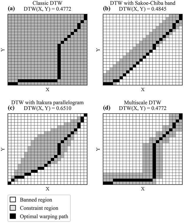
A common approach consists in limiting the time warps by using a constraint region: The set of warping paths is restricted to the set of warping paths such that all their elements belong to the constraint region. This approach also decreases the computational complexity of the cost and accumulated cost matrices since only the entries belonging to the constraint region have to be computed, but adds the computational cost of the constraint region. Two commonly used constraint regions are the Sakoe-Chiba band [9] and the Itakura parallelogram [12]. The Sakoe-Chiba band limits the time warps to be no greater than half the bandwidth, while the Itakura parallelogram limits the time warps to be no greater than a variable value, this value being larger in the middle of the time series than at the starting and ending time points. The Sakoe-Chiba band and the Itakura parallelogram do not depend on the values of the time series, but only on their lengths. Other constraint regions depending on the values of the time series have been proposed [13, 14], relying on the optimal warping path for downsampled versions of the original time series. Figure 1 illustrates the optimal warping path for the original DTW algorithm and three of its variants with constraint regions.

Figure 1.

Dynamic time warping. Illustration of the classic dynamic time warping (DTW) algorithm (a) and three of its variants with a constraint region: DTW with Sakoe-Chiba band (b), DTW with Itakura parallelogram (c), and multiscale DTW (d). For each algorithm, the set of admissible alignments and the optimal warping path is highlighted, and the corresponding score is computed. Multiscale DTW, by computing a constraint region specific to the input time series, is able to retrieve the same warping path as classic DTW with no constraint region.

Another variant of DTW, called soft-DTW [15], replaces the min function, which is not differentiable, with a smooth minimum function, namely the LogSumExp function, which is differentiable. The soft-DTW function, being differentiable, can be used as a loss function for machine learning algorithms, in particular artificial neural networks.

3. Kernel methods

Kernel methods are popular machine learning algorithms allowing for nonlinear transformations or decision functions, among which support vector machines are probably the most famous ones and have been successfully used in numerous applications.

Kernel methods rely on a kernel function measuring similarity between any pair of inputs. A key necessary assumption of kernel methods is that the kernel is positive-definite. However, as mentioned in the previous section, DTW is not a distance because it does not satisfy the triangle inequality, implying that DTW cannot be used to define a positive-definite kernel. Although DTW has been used with kernel methods in several publications with some tricks, the fact that the theoretical assumptions are not satisfied is an important limitation.

A true positive-definite kernel for time series, called the global alignment kernel, was proposed [16]. The global alignment kernel, denoted $k_{\mathit{GA}}^{\gamma }$, is defined as the sum of all the negatively exponentiated costs over all the possible warping paths:

$$\begin{array}{c}{k}_{\mathit{GA}}^{\gamma }\left(X,Y\right)=\sum _{p\in P}\mathit{exp}\left(-C_p\left(X,Y\right)/\gamma \right)\end{array}$$E11

where $C_p\left(x,y\right)$, defined in Eq. (3), is the cost associated with the warping path $p$, $P$ is the set of all the warping paths, and $\gamma >0$ is a smoothing parameter.

It is important to note that the global alignment kernel is not a true kernel for every local divergence $f$. However, it can be proven that, if $1/\left(1+\mathit{exp}\left(f\right)\right)$ is a positive-definite kernel, then $k_{\mathit{GA}}^{\gamma }$ is a kernel. In particular, this condition is satisfied when $f$ is the squared difference function (and more generally the squared Euclidean distance for multivariate time series).

The global alignment kernel has the same computational complexity as DTW, that is, $O\left(\mathit{nm}\right)$, because the score between two time series can be computed using a recurrence equation similar to Eq. (5). Constraint regions such as the Sakoe-Chiba band and the Itakura parallelogram can also be used with global alignment kernels.

Support vector machines with the global alignment kernel have been shown to yield better predictive performances than with other pseudo kernels based on DTW for several multivariate time series classification tasks [16].

4. Shapelet-based algorithms

A shapelet is defined as a subsequence of consecutive observations from a time series. In some use cases, specific shapelets can be characteristic of the classes and thus helpful at discriminating them. Several algorithms rely on shapelets, either by extracting the best shapelets from the training data set or by directly learning them.

4.1 Shapelet transform

Lines and colleagues proposed an algorithm, called Shapelet Transform, that extracts the best shapelets from a data set [17]. Let $X=\left(x_1,\dots ,x_n\right)$ be a time series of $n$ real-valued observations and $S=\left(s_1,\dots ,s_l\right)$ be a shapelet of $l$ real numbers, with $l\le n$. The distance between the shapelet $S$ and the time series $X$, denoted $d\left(S,X\right)$, is defined as the minimum of the squared Euclidean distances between $S$ and all the shapelets of length $l$ from $X$:

$$\begin{array}{c}d\left(S,X\right)=\underset{j\in \left\{0,\dots ,n-l\right\}}{\mathit{min}}\sum _{i=1}^l{\left(s_i–x_{j+i}\right)}^2\end{array}$$E12

The algorithm extracts all the shapelets whose length belongs to a range, the range being a hyperparameter of the algorithm, and selects the $k$ best shapelets, $k$ being another hyperparameter of the algorithm. This process can be seen as univariate feature extraction, where each feature is the distance between a given shapelet and all the time series in the data set. The shapelets are ranked based on the F-statistics of the analysis of variance test that compares the between- and within-class variabilities. In order to extract features (i.e., shapelets) that are not highly correlated, self-similar shapelets are removed, with any pair of shapelets being considered self-similar if they are from the same time series and have any overlapping indices.

When the $k$ best shapelets have been identified and the corresponding features have been generated, any standard machine learning classifier can be applied to this new data set. Lines and colleagues investigated eight classifiers, including one-nearest neighbor classifier, support vector machine with a linear kernel, and random forest. In their experiments, the support vector machine with a linear kernel yielded the best results on average.

One limitation of this algorithm is its computational complexity. For a data set of $N$ time series of length $n$, there are $N\times \left(n–l+1\right)$ shapelets of length $l$. Since many values of $l\in \left\{1,\dots ,n\right\}$ are investigated, the maximal computational complexity is $O\left(N\times n^2\right)$. Moreover, the definition of self-similarity for shapelets does not take into account the values of the shapelets, meaning that two shapelets very similar in terms of Euclidean distance but extracted from two different time series are not considered self-similar, even though they yield very similar features.

Several modifications to the algorithm have been proposed such as using other criteria to rank shapelets [18], in particular for multi-class classification tasks [19], and other classifiers built on top of the transformation [18].

4.2 Learning shapelets

In order to address the limitations of the Shapelet Transform algorithm, another algorithm relying on learning shapelets, instead of extracting them, was proposed [20].

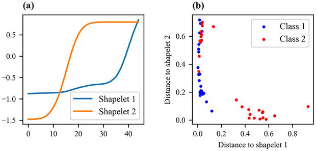
The distance between a shapelet and a time series defined in Eq. (12) relies on the minimum function, which is not differentiable. Similar to the soft-DTW variant of DTW, the minimum function is replaced with a smooth minimum function, namely the LogSumExp function, which is differentiable. The logistic regression algorithm is used as the machine learning classifier built on top of the transformation. Figure 2 illustrates two learned shapelets and the distances between both shapelets and time series, highlighting that each shapelet is characteristic of one class.

Figure 2.

Shapelets. Two shapelets have been learned from a training data set (a) and the distances between both shapelets and the training time series are plotted (b). The first shapelet is really specific of the second class, while the second shapelet is present in all the time series belonging to the first class and in some time series belonging to the second class.

Since both the transformation and classification functions are differentiable, the chain rule allows for computing the gradients of the objection function with respect to the shapelets and the logistic regression coefficients, respectively, thus minimizing the objective function can be attempted to be solved by gradient descent.

Learning shapelets instead of extracting them has several advantages. First, it may lead to shapelets that are not from the data set but are discriminative of the classes. Second, it does not require going through the whole data set, and thus may be faster to train, especially with stochastic variants of gradient descent.

Nonetheless, learning shapelets also comes with drawbacks. As both the shapelets and the logistic regression coefficients need to be learned, the objective function is not convex (one can see the analogy with some clustering algorithms, such as $k$-means and Gaussian mixture models, where both the parameters and the members of the clusters need to be learned). Therefore, the optimization algorithm may converge to a bad local minimum. It also leads to more hyperparameters as the optimization process is a key component of the algorithm. Finally, as learning shapelets is embedded into the algorithm, it may not be optimal to try other classifiers than logistic regression later on, whereas the Shapelet Transform algorithm is independent of the machine learning classifier, and thus, the transformation step can be computed only once and many classifiers can be built on top of it to find the best performing classifier.

5. Tree-based algorithms

Standard tree-based machine learning algorithms, such as random forest [21] and extremely randomized trees [22], are popular algorithms that have proven to be powerful. The use of such algorithms for time series classification has been investigated, ranging from extracting features used as input to modifying the construction of each tree in the ensemble.

5.1 Time series forest

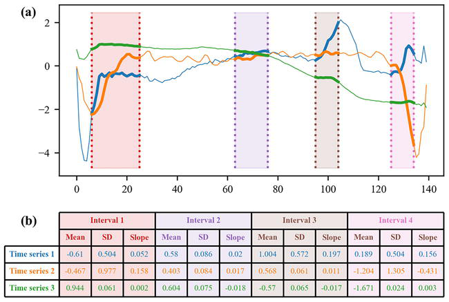
One of the first proposed algorithms based on the random forest algorithm is called time series forest [23] and is relatively simple. The algorithm considers information from subsequences of the time series. Given a minimum length for the subsequences, which is a hyperparameter, random intervals are generated, with the start indices, end indices, and lengths of all the intervals being all randomly generated. For a given time series and a given interval, the corresponding subsequence is the ordered set of values from the time series belonging to the interval. From each subsequence, three features are extracted: the mean, the standard deviation, and the slope. Figure 3 illustrates this feature extraction.

Figure 3.

Time series forest. Random intervals are generated and the corresponding subsequences from each time series are extracted (a). Three features are derived from each subsequence: The mean, the standard deviation (SD), and the slope (b).

The total number of extracted features is thus three times the number of considered intervals. A random forest classifier is then trained on these extracted features. Predictions for new time series are obtained in the same manner: Given the already generated intervals, the three features are extracted from each subsequence, then the fitted random forest classifier outputs its prediction.

5.2 Time series bag-of-features

Time series bag-of-features [24] is a more advanced algorithm also based on features extracted from subsequences and random forest.

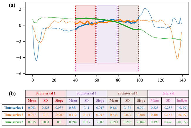
First, time series bag-of-forest also randomly generates intervals. However, this algorithm extracts more features than time series forest. Each interval is divided into non-overlapping subintervals, and the same three features (mean, standard deviation, and slope) are extracted from the subsequences corresponding to each subinterval. Moreover, four features from each interval are also extracted: the mean and the standard deviation of the subsequence corresponding to this interval, as well as the start and end indices of this interval. Figure 4 illustrates this feature extraction.

Figure 4.

Time series bag-of-features. Random intervals are generated and each window is split into subintervals, from which subsequences are extracted (a). Three features are derived from the subsequences of each subinterval (the mean, the standard deviation (SD), and the slope) and four features are derived from the subsequences of each interval (the mean, the standard deviation (SD), and the start and end indices) (b).

A new data set is created, whose samples are the subsequences extracted from the time series for every interval, and whose features are the aforementioned extracted features. In this new data set, the number of samples is thus the number of time series times the number of intervals, while the number of features is equal to four plus three times the number of subintervals (four features for the interval and three features for each subinterval in the interval). The class of each subsequence is defined as the class of the time series from which the subsequence was extracted.

Then, a first random forest classifier is trained on this new data set, then outputs the probabilities to belong to each class for each subsequence. During the training phase, out-of-bag probabilities are actually used to have unbiased estimates of probabilities; that is, only trees that were built on bootstrap samples that did not contain the subsequence are used to compute the probabilities. Then, the probabilities are binned in order to summarize the distribution of the probabilities over all the subsequences; that is, the histogram of probabilities is computed to identify, for each class, how many subsequences were given high probabilities to belong to this class. More precisely, for each time series and for each class, the (out-of-bag) probabilities of belonging to the given class for all the subsequences extracted from the given time series are binned. For each time series and for each class, the mean probability over all the subsequences is also computed. Performing this operation for each time series and each class creates a new data set whose samples are the time series and whose features are the mean and binned probabilities for each class over all the subsequences.

Finally, a second random forest classifier is trained on this new data set during the training phase and outputs the predicted class for an unseen time series during the inference phase.

5.3 Proximity forest

In contrast to the time series forest and time series bag-of-features algorithms that rely on extracting features from time series and then build a random forest, the proximity forest algorithm [25] works directly with raw time series and is inspired by the extremely randomized trees algorithm.

To better understand the proximity forest algorithm, we briefly recall the main concepts of the extremely randomized trees algorithm. Like in a random forest, several trees are independently trained. The major difference between both algorithms comes from the splitting criterion used to split a node into child nodes. In a random forest, only a random subset of the features is considered, and the best (feature, threshold) pair is chosen over all the possible (feature, threshold) pairs. In extremely randomized trees, randomness goes one step further: Instead of considering all the possible thresholds for each feature from the random subset of features, a single threshold is randomly generated for each feature, and the best (feature, threshold) pair is chosen. The node splitting process is thus much faster in extremely randomized trees since much fewer (feature, threshold) pairs are considered. Another consequence is that a single tree from extremely randomized trees usually performs worse than a single tree in a random forest, but the extremely randomized trees are less correlated than the trees of a random forest, thus benefitting more from averaging the predictions of each tree.

The proximity forest algorithm is heavily inspired by the extremely randomized trees algorithm, the only difference being the splitting criterion that we now describe. In standard decision trees, the splitting criterion is a (feature, threshold) pair that splits a set of samples into two subsets: The subset of samples whose values for the given feature are greater than the threshold, and the subset of samples whose values for the given feature are lower than the threshold. In a proximity forest, the splitting criterion is a (metric, set of exemplars) pair: The metric allows for measuring similarity between any pair of time series, and the set of exemplars is a set containing one exemplar of each class from all the time series belonging to the given node. The number of (metric, set of exemplars) considered at each splitting node is a hyperparameter of the algorithm. Like in extremely randomized trees, the metric and the set of exemplars are randomly chosen: The metric is chosen uniformly at random from a set of 11 metrics for time series, and the exemplar for each class is chosen uniformly at random from all the time series belonging to this class and this node.

Because only a small set of (metric, set of exemplars) pairs is considered at each splitting node and because the decision tree growing process exponentially decreases the sample size at each depth of the tree, the proximity forest is highly scalable to large data sets of time series (in terms of both the number of time series and the number of time points). Because the trees of the proximity forest tend not to be highly correlated, the proximity forest benefits from aggregating the predictions of each tree by decreasing the variance of the final model and has proven to give a good predictive performance on average.

6. Bag-of-words (dictionary-based) approaches

Bag-of-words approaches, also known as dictionary-based approaches, consists in discretizing time series into sequences of symbols, then extracting words from these sequences with a sliding window, and finally counting the number of words for all the words in the dictionary. These approaches are split into two groups: the ones based on discretizing raw time series, and the other ones based on discretizing Fourier coefficients.

6.1 Approaches based on discretizing raw time series

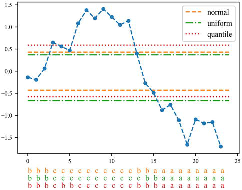
The most commonly used algorithm to discretize raw time series is called Symbolic Aggregation approXimation (SAX) and simply maps each real-valued observation of the time series to its corresponding bin [26]. Several strategies to compute the bin edges are possible: quantiles of the standard normal distribution if the time series was standardized (zero mean, unit variance), uniform bins based on the extreme values of the time series, or quantiles of the time series. Figure 5 illustrates the SAX discretization with different strategies to compute the bins.

Figure 5.

Symbolic aggregate approXimation. A time series is discretized using bin edges. Different strategies to compute the bin edges are possible: Quantiles of the standard normal distribution, uniform bins based on the extreme values of the time series or quantiles of the time series. The resulting sequences of symbols for each strategy are shown at the bottom.

Based on the SAX discretization of standardized time series with quantiles of the standard normal distribution, the bag-of-patterns algorithm [27] uses a sliding window to extract words from the discretized time series and computes the corresponding histogram; that, is the frequency of each word is computed, resulting in a new data set in which each feature is a word from the dictionary and each value is the number of occurrences of the given word in a given time series. Since consecutive subsequences are likely to be very similar and thus lead to identical words, it was proposed to count a single occurrence of identical consecutive words, this process being called numerosity reduction. Finally, a nearest-neighbor classifier was built on top of this transformation to perform classification.

Another algorithm, called Symbolic Aggregation approXimation in Vector Space Model (SAX-VSM), was later proposed with two major differences from the bag-of-patterns algorithm [28]. First, the order of the preprocessing steps is changed. The sliding window is applied to the raw time series to extract subsequences. Each subsequence is standardized and discretized using the SAX algorithm, resulting in an ordered sequence of words, to which numerosity reduction is usually applied. Second, classification is based on a simple numerical statistic used in natural language processing: the term frequency—inverse document frequency (TF-IDF) matrix. The idea is to identify words that are specific to each class. After computing the frequency of each word in the dictionary for each time series (resulting in a vector for each time series), all the vectors corresponding to time series belonging to the same class are summed in order to obtain the frequency of each word for each class. This process results in the term frequency matrix, whose rows represent the words in the dictionary, the columns represent the classes in the data set, and each entry is the frequency of the given word for the given class. Each row of this matrix is then normalized by the number of classes in which the word is present so that words that are specific to a small number of classes are more heavily weighted than words present in many classes. This normalized matrix is the so-called TF-IDF matrix. Classification is performed using the cosine similarity between the word frequency vector of a new time series and each column of the TD-IDF matrix, the predicted class being the one yielding the highest cosine similarity.

6.2 Methods based on discretizing Fourier coefficients

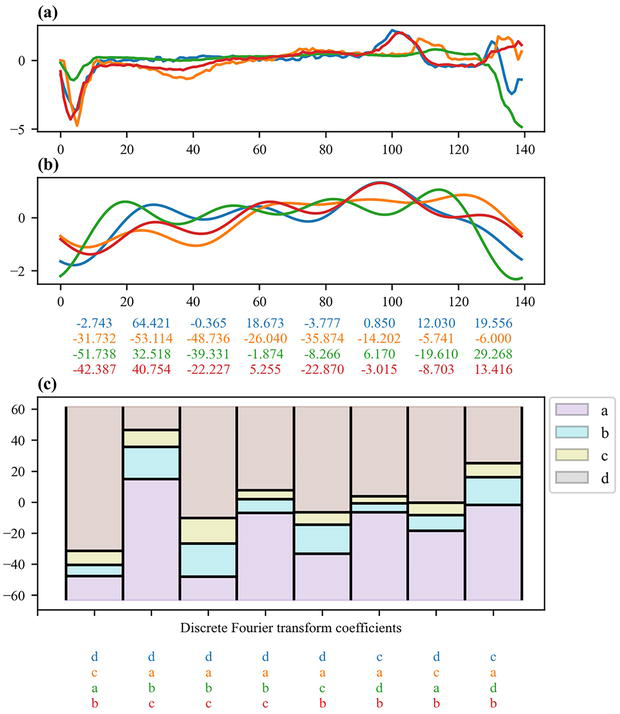
Instead of discretizing raw time series, other methods rely on discretizing Fourier coefficients. The most commonly used algorithm to do so is called Symbolic Fourier Approximation (SFA) and is a two-stage algorithm [29]. In the first stage, the discrete Fourier transform of the time series is computed and a subset of the Fourier coefficients is kept. In unsupervised learning, this subset is usually the set of first coefficients (the ones corresponding to the lowest frequencies) since they represent the trend of the time series. In supervised learning, univariate feature selection can be applied in order to select the more highly ranked coefficients based on statistics such as the F-statistics returned by one-way analysis of variance tests. Importantly, the same Fourier coefficients must be selected for all the time series. This transformation results in a matrix whose rows are time series and whose columns (i.e., features) are Fourier coefficients. In the second step, each column of this matrix is independently discretized. In unsupervised learning, the bin edges are usually computed so that the bins are uniform (i.e., the bin edges are based on the extreme values of the Fourier coefficients) or the number of Fourier coefficients falling in each bin is the same (i.e., the bin edges are based on the quantiles of the Fourier coefficients). In supervised learning, the bin edges can be computed to minimize an impurity criterion such as entropy. Therefore, the SFA algorithm transforms a time series into a single sequence of symbols (i.e., a single word). Figure 6 illustrates the SFA transformation.

Figure 6.

Symbolic Fourier approximation. Raw time series (a) are approximated using a subset of the coefficients of the discrete Fourier transform, with the values of the coefficients for each time series being displayed at the bottom (b). The coefficients are discretized using bin edges that are computed either as uniform bins based on the extreme values of the Fourier coefficients or as quantiles of the Fourier coefficients, and the resulting sequences of symbols are displayed at the bottom (c).

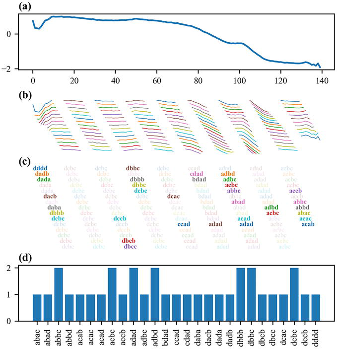
Based on the SFA transformation, the Bag-of-SFA-Symbols (BOSS) algorithm was proposed [30]. First, subsequences of a time series are extracted with a sliding window and the SFA transformation is applied to each subsequence, resulting in an ordered sequence of words. Numerosity reduction is often applied to this sequence to avoid outweighing stable sections of time series. The frequency of each word is computed to obtain the word histogram of the time series. Figure 7 illustrates these stages of the BOSS algorithm. Finally, classification is performed using the nearest-neighbor algorithm with the BOSS metric, which is a variant of the squared Euclidean distance that does not take into account the words that are not present in the histogram of the first time series. An ensemble of BOSS classifiers with sliding windows of different lengths is usually built to capture patterns of different lengths.

Figure 7.

Bag-of-SFA symbols. From a raw time series (a), a sliding window is applied to extract subsequences (b). Each subsequence is transformed into a word using the symbolic Fourier approximation (SFA) algorithm, and only the first occurrence of identical back-to-back words is kept (c). Finally, the histogram of the bag of words (i.e., the frequency of each word) is computed (d).

Several extensions of the BOSS algorithm have been proposed.

The Bag-of-SFA-Symbols in Vector Space (BOSSVS) combines the BOSS and vector space models [31]. Similar to some modifications of the bag-of-patterns algorithm in SAX-VSM, a single histogram is computed for each class (instead of a histogram for each time series) and the TF-IDF matrix is computed. Classification is performed by finding the class yielding the highest cosine similarity between the histogram of the time series and the TF-IDF vector of each class.

Randomized BOSS (RBOSS) introduces randomization in the choice of the lengths of the sliding windows and uses a more sophisticated aggregation of the predictions of the base BOSS classifiers, leading to lower computational time while maintaining similar performance [32].

BOSS with Spatial Pyramids (SP-BOSS) makes use of spatial pyramids, a method commonly used in computer vision, in order to combine temporal and phase independent features, and replaces the BOSS metric with the histogram intersection metric [33].

The Word Extraction for Time Series Classification (WEASEL) algorithm extends BOSS by integrating the sliding windows of different lengths inside the transformation, thus before the classification step [34]. To decrease the size of the resulting dictionary, only non-overlapping subsequences are extracted for each sliding window and the chi-squared test is applied to filter in the most relevant features. Since the constructed input matrix of word counts may have many features and be very sparse, logistic regression is built on top of the WEASEL transformation as this algorithm can handle both characteristics. WEASEL plus Multivariate Unsupervised Symbols and Derivatives (WEASEL+MUSE) is an extension of WEASEL to multivariate time series classification [35].

The Temporal Dictionary Ensemble (TDE) algorithm combines design features of four of these algorithms (BOSS, RBOSS, SP-BOSS, and WEASEL) with a novel mechanism of base classifier model selection based on an adaptative form of Gaussian process modeling of the parameter space [36].

7. Imaging time series

In order to investigate temporal correlations between all the pairs of observations, several methods relying on transforming time series (i.e., vectors) into images (i.e., matrices) have been proposed. In this section, we focus more on presenting these transformations than the classification algorithms built on top of them. Since these classifiers often belong to the class of deep learning algorithms, they will be more detailed in the next section.

7.1 Recurrence plot

A recurrence plot is an old technique that was originally introduced to visually inspect time constancy in dynamical systems through trajectories [37]. A trajectory is defined as a subsequence of equally spaced values:

$$\begin{array}{c}\forall i\in \left\{1,\dots ,n-\left(m-1\right)\tau \right\},\overrightarrow{x_i}=\left(x_i,x_{i+\tau },\dots ,x_{i+\left(m-1\right)\tau }\right)\end{array}$$E13

where $m$ is the length of the trajectory and $\tau$ is the time delay, that is, the time gap between back-to-back time points in the trajectory.

A recurrence plot, denoted by $R$, is a matrix consisting of the binarized pairwise distances between all the pairs of trajectories from a time series:

$$\begin{array}{c}\forall i,j\in \left\{1,\dots ,n-\left(m-1\right)\tau \right\},R_{i,j}=\Theta \left(\epsilon -{‖\overrightarrow{x_i}-\overrightarrow{x_j}‖}_2\right)\end{array}$$E14

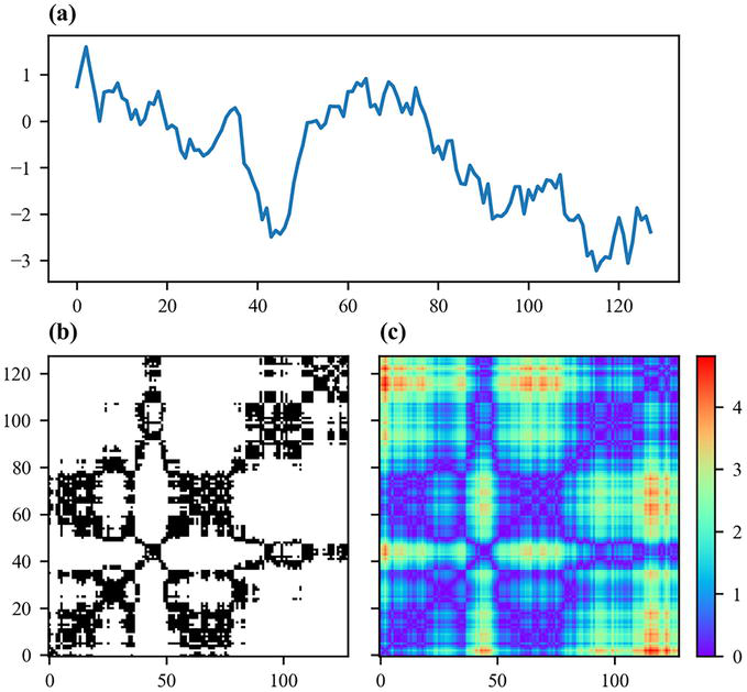
where $\epsilon$ is the threshold used to binarize the distance and $\Theta$ is the Heaviside step function, which is 1 for positive arguments and 0 for non-positive arguments. Visually, as a black-and-white image, a pixel is black if and only if the distance between the two considered trajectories is smaller than the threshold (Figure 8).

Figure 8.

Recurrence plot. Starting from a time series (a), the Euclidean distances between all the pairs of trajectories are computed and binarized using a threshold (b). The thresholding step is sometimes skipped and the raw pairwise Euclidean distances are considered (c).

Recurrence plots have been used as a preprocessing step to classify time series. Silva and colleagues used a $k$-nearest neighbor classifier with the Campana-Keogh distance [38] to measure the similarity between recurrence plots [39]. Tamura and colleagues used the recurrence plots computed from moving average convergence divergence histograms to train an artificial neural network consisting of stacked auto-encoders [40]. Hatami and colleagues trained a 2D convolutional neural network using as input non-binarized recurrence plots by skipping the thresholding step, resulting in grayscale texture images [41].

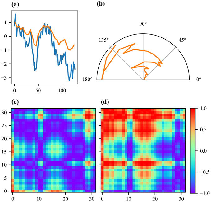
7.2 Gramian angular field

While recurrence plots consider phase space trajectories, another method, called the Gramian angular field and based on the polar coordinate representation of time series, was proposed [42].

A time series $X=\left(x_1,\dots ,x_n\right)$ of real-valued observations is first linearly rescaled into the range $\left[a,b\right]$ with $-1\le a<b\le 1$:

$$\begin{array}{c}\forall i\in \left\{1,\dots ,n\right\},\stackrel{\sim }{x_i}=a+\left(b-a\right)\times \frac{x_i-\mathit{min}\left(x\right)}{\mathit{max}\left(x\right)-\mathit{min}\left(x\right)}\end{array}$$E15

The values of $a$ and $b$ may depend on the time series if the scale of the time series is important. Otherwise, the range is usually $\left[a,b\right]=\left[-1,1\right]$ or $\left[a,b\right]=\left[0,1\right]$.

The rescaled time series $\stackrel{\sim }{X}$ is then represented in polar coordinates with the radii depending on the time points and the angles depending on the values of the rescaled time series:

$$\begin{array}{c}\forall i\in \left\{1,\dots ,n\right\},r_i=\frac{i}{n}\end{array}$$E16

$$\begin{array}{c}\forall i\in \left\{1,\dots ,n\right\},{\varphi }_i=\mathit{arccos}\left(\stackrel{\sim }{x_i}\right)\end{array}$$E17

Only the angles are considered since the radii do not depend on the values of the time series.

A Gramian angular field measures temporal correlation by computing the trigonometric sum or difference between all the pairs of angles. When the trigonometric sum is applied, the Gramian angular field is called a Gramian angular summation field, while it is called a Gramian angular difference field when the difference is applied. Let $\mathit{\text{GASF}}$ be the matrix of a Gramian angular summation field and then $\mathit{\text{GADF}}$ the matrix of a Gramian angular difference field. The entries of both matrices are computed using the following equations:

$$\begin{array}{c}\forall i,j\in \left\{1,\dots ,n\right\},\mathit{GAS}{F}_{i,j}=\mathit{cos}\left({\varphi }_i+{\varphi }_j\right)\end{array}$$E18

$$\begin{array}{c}\forall i,j\in \left\{1,\dots ,n\right\},\mathit{GAD}{F}_{i,j}=\mathit{sin}\left({\varphi }_i-{\varphi }_j\right)\end{array}$$E19

Figure 9 summarizes the whole process to generate Gramian angular fields and illustrates both the Gramian angular summation and difference fields. By default, a Gramian angular field is an $n\times n$ matrix, which can be excessively large for large $n$. A common approach consists in first downscaling the time series from $n$ points to $m$ points, with $m$ being the desired size of the Gramian angular fields. It should also be noted that the computation of Gramian angular fields can be simplified using trigonometric identities:

Figure 9.

Gramian angular fields. A raw time series is normalized in range [−1, 1] (a) and is represented in polar coordinates (b). The Gramian angular fields are computed either as the cosine of the sum (c) or the sine of the difference (d) of all the pair of angles.

$$\forall i,j\in \left\{1,\dots ,n\right\},\mathit{GAS}{F}_{i,j}=\stackrel{\sim }{x_i}\stackrel{\sim }{x_j}-\sqrt{\left(1-\stackrel{\sim }{x_i}\right)\left(1-\stackrel{\sim }{x_j}\right)}$$E20

$$\begin{array}{c}\forall i,j\in \left\{1,\dots ,n\right\},\mathit{GAD}{F}_{i,j}=\stackrel{\sim }{x_j}\sqrt{1-\stackrel{\sim }{x_i}}-\stackrel{\sim }{x_i}\sqrt{1-\stackrel{\sim }{x_j}}\end{array}$$E21

Gramian angular fields have been used for time series classification as a preprocessing step to generate images used as input of a tiled convolutional neural network [42] and of the pre-trained Inception v3 model followed by a multilayer perceptron [43].

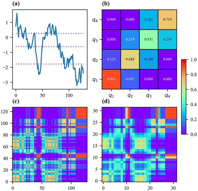
7.3 Markov transition field

Another method consists in assimilating a time series, after discretization, as a Markov chain, and is called Markov transition field [42].

A time series $X=\left(x_1,\dots ,x_n\right)$ of real-valued observations is first discretized based on its quantile bins; that is, each $x_i$ is assigned to its corresponding bin $q_j$ with $j\in \left\{1,\dots ,Q\right\}$ and $Q$ being the number of quantile bins, resulting into a discretize-valued time series of length $n$. By considering this discretize-valued time series as observations of a first-order Markov chain, one can compute the number of occurrences of pairs of back-to-back bins for every pair of bins, resulting in a $Q\times Q$ matrix. This matrix is then normalized to transform the frequencies into probabilities, leading to the Markov transition matrix, whose entries give the probabilities of going from $q_j$ to $q_k$ for every pair $\left(q_j,q_k\right)$ of bins.

The Markov transition matrix is insensitive to the temporal distribution of the time series $X$ since it only captures the frequencies of the transition, but not at which time points they occurred. Moreover, its size depends on the number of bins and not the length of the time series, although larger time series may allow for a larger number of bins. To overcome these issues, the Markov transition matrix is projected onto a $n\times n$ matrix that is called the Markov transition field.

Let $\mathit{MTF}$ be a Markov transition field and $q$ be the function that maps the real-valued observations of the time series into their bins. Each entry of the Markov transition field is an entry of the Markov transition matrix, and thus a transition probability. $\mathit{MT}{F}_{i,j}$, that is, the Markov transition field entry for the pair $\left(x_i,x_j\right)$, is the probability of going from the bin associated to $x_i$, that is, $q\left(x_i\right)$, to the bin associated to $x_j$, that is, $q\left(x_j\right)$:

$$\begin{array}{c}\forall i,j\in \left\{1,\dots ,n\right\},\mathit{MT}{F}_{i,j}=\mathbb{P}\left(q\left(x_j\right)|q\left(x_i\right)\right)\end{array}$$E22

Figure 10 summarizes the whole process to generate Markov transition fields from raw time series. By default, a Markov transition field is an $n\times n$ matrix, which can be excessively large for large $n$. There are two common approaches to address this issue. The first approach consists in first downscaling the time series from $n$ points to $m$ points, with $m$ being the desired size of the Markov transition fields, as it is done for Gramian angular fields. The second approach consists in downscaling the Markov transition field itself, from $n\times n$ to $m\times m$, by taking the mean value of each submatrix, which is commonly referred to as average pooling in the deep learning literature.

Figure 10.

Markov transition field. A raw time series is discretized with bin edges being defined as quantiles of the time series (a). The discretized time series is seen as a first-order Markov chain and the corresponding Markov transition matrix, representing the probability of going from a given bin to another given bin, is computed (b). The Markov transition matrix is spread through time to obtain the Markov transition field (c). The size of the Markov transition field can be reduced by taking the mean value inside each submatrix (d).

Like Gramian angular fields, Markov transition fields have been used for time series classification as a preprocessing step to generate images then train a tiled convolutional neural network [42].

8. Deep learning

Over the past decade, deep learning has led to many breakthroughs in several fields such as computer vision and natural language processing. Deep learning has also been recently investigated for time series classification. We refer the readers to an exhaustive review on this specific topic [44] and present only the major contributions in this review.

Ismail Fawaz and colleagues [45] proposed an ensemble of 60 neural network models to perform time series classification. The 60 models come from 6 architectures: a multi-layer perceptron [46], a fully convolutional neural network [46], a residual network [46], an encoder [47], a multi-channel deep convolutional neural network [48], and a time convolutional neural network [49]. Each architecture is used to train 10 different models with different initial weight values.

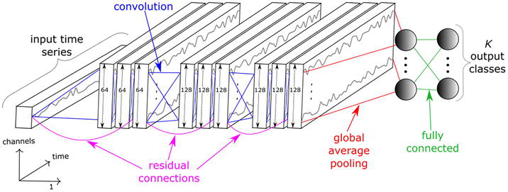
InceptionTime [50] is probably the main deep learning model for time series classification. InceptionTime is a neural network ensemble consisting of five Inception networks. Figure 11 illustrates the architecture of each Inception network, consisting of blocks of three Inception modules (6 blocks by default), followed by a global averaging pooling layer and a fully-connected layer with the softmax activation function. Each Inception module consists of convolutions with kernels of several sizes followed by batch normalization and the rectified linear unit activation function.

Figure 11.

InceptionTime architecture. The InceptionTime artificial neural network consists of several inception modules with residual connections, followed by a global average pooling layer and a fully connected layer. Reproduced from Ref. [50].

Other investigations of deep learning for time series classification include transfer learning [51], data augmentation [52], adversarial attacks [53], and neural architecture search [54].

9. Random convolutions

Convolutional neural networks, containing several convolutional layers, have been investigated for time series classification. The values of the convolutional layers are trainable parameters that are optimized by stochastic gradient descent or a variant thereof. Convolutional neural networks have a large number of trainable parameters in comparison with more classic algorithms such as logistic regression or support vector machines, thus usually requiring a large sample size to find good values for the trainable parameters.

Based on this observation, the Random Convolutional Kernel Transform (ROCKET) algorithm was proposed [55]. This algorithm extracts features from time series using a large number of random convolutional kernels, meaning that all the parameters of all the kernels (length, weights, bias, dilation, and padding) are randomly generated from fixed distributions. Instead of extracting a single feature for each kernel, such as the maximum or the mean, as it is usually performed in convolutional neural networks, two features are extracted: the maximum and the proportion of positive values.

The classifier built on top of the transformation is responsible for selecting the most relevant features to perform classification. A ridge regression classifier was originally proposed for several reasons. First, it is highly efficient when the number of classes is high, because the multiclass classification task is treated as a multi-output regression task, with the predicted class corresponding to the output with the highest value; thus, the projection matrix needs to be computed only once. Second, the optimization of the $\lambda$ parameter (controlling the amount of regularization) using leave-one-out cross-validation is also highly efficient [56]. Logistic regression was rather used for data sets in which the number of training time series was much larger than the number of extracted time series due to the better scalability of logistic regression solved with stochastic gradient descent for large numbers of training samples.

The ROCKET algorithm combined with a linear classifier has a much lower computational complexity than the best-performing time series classification algorithms while having a comparable performance. Its reported performance is actually higher on average than the ones of convolutional neural networks on the commonly benchmarked data sets. Given its high predictive performance and low computational time, ROCKET is one of the most prominent transformation algorithms for time series classification.

Several recent extensions have been proposed. MiniROCKET [57] reduces the randomness of the parameters of the kernels by using a fixed value or sampling from smaller distributions. Moreover, it only extracts the proportion of positive values for each kernel. These modifications also allow for more optimization and lead to a much lower computational complexity while maintaining similar performance. MultiROCKET [58] extends MiniROCKET by extracting possibly several features, leading to a slightly higher computational time but better accuracy. In particular, the authors found that the proportion of positive values and the longest period of consecutive positive values are the most effective features to be extracted from time series convolutional outputs.

10. Ensemble models

Averaging the predictions of several independently trained models into a single prediction is a common approach to build a better final model by decreasing the variance of the predictions. In traditional ensemble methods, all the base classifiers belong to a given type of algorithms. For instance, in a random forest, all the base classifiers are decision trees. However, using a single type of algorithm limits the upsides and downsides of the final model to the ones of the base classifier. On the other hand, using several types of algorithms allows for learning a more diverse representation of the data. In particular, for time series classification, ensemble models that combine different types of algorithms (bag-of-words approaches, shapelet-based algorithms, convolutions, etc.) have been developed. They often are state-of-the-art in terms of predictive performance, at the cost of high computational complexity.

The Collective of Transformation-Based Ensembles (COTE) algorithm was the first proposed ensemble classifier [59]. The most effective ensemble strategy was found to combine all the classifiers into a flat hierarchy and the corresponding model is often referred to as Flat-COTE [60]. Flat-COTE combines 35 classifiers over four data representations: 11 classifiers based on whole series similarity measures, 8 classifiers based on shapelet-transform, 8 based on autocorrelation features, and 8 based on power spectrum.

The Hierarchical Vote Collective of Transformation-Based Ensembles (HIVE-COTE) algorithm is an extension of COTE with significant modifications [60], including a new type of spectral classifier called Random Interval Spectral Ensemble, two more classifiers (BOSS and Time Series Forest), and a hierarchical voting procedure, defined as a weighted average of the probabilities returned by each classifier, with the weights being proportional to the classification accuracy estimated through cross-validation. HIVE-COTE is often updated based on newly published algorithms, with versions 1.0 [61] and 2.0 [62] being recently published.

The Time Series Combination of Heterogeneous and Integrated Embedding Forest (TS-CHIEF) algorithm is another ensemble model rivaling with HIVE-COTE in terms of predictive performance while having a substantially lower runtime [63]. TS-CHIEF builds a random forest of decision trees whose splitting functions are time series specific and based on similarity measures, dictionary (bag-of-words) representations, and interval-based transformations.

11. Public data sets and open-source software

So far, we have presented the mathematical aspects of time series classification algorithms. However, in practice, implementations and evaluations of these algorithms are equally important. In this section, we briefly present the commonly used data sets to assess the performance of time series classification algorithms, and popular software making available implementations of such algorithms.

11.1 Public data sets

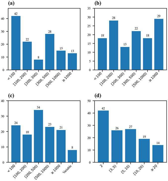
The main resource used to benchmark time series classification algorithms is the UCR Time Series Classification Archive [64, 65], providing public access to univariate time series classification data sets that are already split into training and test sets, leading to a consistent benchmarking between algorithms. The current version of the archive contains 128 data sets from various domains (audio, medicine, motion, sensor, simulation, spectroscopy, etc.). Figure 12 presents the distribution of several variables (number of time series in the training and test sets, number of time points, and number of classes) over the 128 data sets.

Figure 12.

Descriptive statistics of the data sets in the UCR time series classification archive. The UCR time series classification archive provides 128 univariate time series classification data sets. The histograms of four features of these data sets are plotted: The number of training time series (a), the number of test time series (b), the number of time points (c), and the number of classes (d).

For multivariate time series classification algorithms, the main benchmark resources are the UEA Multivariate Time Series Classification Archive [66] and a publicly available archive [67], with some data sets being available in both resources.

A website [68] provides useful information about the data sets, the algorithms, and the performance of these algorithms on all the data sets, as well as download links for the data sets in the UCR & UEA Time Series Classification Repository.

11.2 Open-source software

Another key element of scientific research in machine learning is code availability. Although the code of most of the algorithms presented in this review is provided by their original authors, it is not trivial, for a new user, to build their work on top of it for several reasons. First, the code is usually only organized in order to reproduce the experiments (i.e., obtaining the same performance for all the data sets included in the analysis). Second, the code is usually neither commented nor documented. Third, different authors may code in different programming languages. For instance, among the algorithms presented in this review, the programming languages used in their original implementations included Java, Python, and R. All of these reasons make, for a given user, reusing the provided code and comparing different algorithms difficult.

Open-source software aims at providing, under the same application programming interface, a variety of tools, including implementations of specific algorithms, preprocessing tools, data set fetching and loading utilities, and visualization tools, all being documented, with the source code being publicly available. Popular open-source libraries for general machine learning already exist, such as scikit-learn [69] in Python and caret [70] in R. Several open-source libraries, focused on time series classification to different extents, have been developed, most of them being Python packages, which is not surprising as Python has become one of the most popular programming languages for machine learning.

Pyts [71] is a Python package entirely dedicated to time series classification, providing implementations of many algorithms presented in this review. Sktime [72] and tslearn [73] are more general machine learning toolboxes for time series, providing tools for other types of machine learning such as forecasting and clustering. Nonetheless, sktime also provides implementations for a lot of time series classification algorithms.

Table 1 enumerates the time series classification algorithms made available in the following libraries: pyts, sktime, and tslearn. Pyts and sktime separate themselves from tslearn by the numerous implemented algorithms in both Python packages. Research on deep learning approaches is recent, and the fact that it is developed in other libraries and that it is computationally intensive while not being the current state-of-the-art may explain that the development of dedicated libraries is lacking behind.

Category	Algorithm	pyts	sktime	tslearn
Metrics	k-nearest neighbors classifier with dynamic time warping	✓	✓	✓
Kernels	Support vector machines with global alignment kernel	✗	✗	✓
Shapelets	Shapelet transform	✓	✓	✗
	Learning shapelet	✓	✗	✓
Tree-based	Time series forest	✓	✓	✗
	Time series bag-of-features	✓	✗	✗
	Proximity forest	✓	✓	✗
Bag-of-words	Bag-of-patterns	✓	✗	✗
	SAX-VSM	✓	✗	✗
	BOSS	✓	✓	✗
	BOSSVS	✓	✗	✗
	WEASEL	✓	✓	✗
	WEASEL+MUSE	✓	✓	✗
	Randomized BOSS	✗	✓	✗
	BOSS with spatial pyramids	✗	✗	✗
	Temporal dictionary ensemble	✗	✓	✗
Image	Recurrence plot	✓	✗	✗
	Gramian angular field	✓	✗	✗
	Markov transition field	✓	✗	✗
Deep learning	Multilayer perceptron	✗	✓	✓
	Residual network	✗	✓	✗
	InceptionTime	✗	✓	✗
Random convolutions	ROCKET	✓	✓	✗
	MiniROCKET	✗	✗	✗
	MultiROCKET	✗	✗	✗
Ensemble	COTE	✗	✗	✗
	HIVE-COTE	✗	✗	✗
	HIVE-COTE version 1.0	✗	✓	✗
	HIVE-COTE version 2.0	✗	✓	✗
	TS-CHIEF	✗	✗	✗

Table 1.

Availability of time series classification algorithms in open-source libraries.

For each algorithm, the availability of an implementation in the main libraries dedicated to time series classification is provided. Pyts and sktime, in addition to their documentation and unit tests, provide implementations of many algorithms under a unified application programming interface. Versions of the libraries: pyts (0.13.0), sktime (0.24.1), and tslearn (0.6.3).

Other noteworthy software for time series classification includes the Python packages seglearn [74], tsfresh [75], and cesium [76], although these libraries do not provide implementations of many specific time series classification algorithms published in the literature, as well as the Java library tsml [77], which provides a lot of benchmarking results, but is mostly oriented toward academic research as it is neither tested nor documented yet.

12. Conclusion

Over the last decades, a lot of research on time series classification has led to major improvements in terms of predictive performance and scalability. Many approaches have been investigated, ranging from specific metrics to simple and complex feature extraction and transformations. More recently, open-source libraries dedicated to time series classification have been developed in order to provide implementations of these algorithms under a unified application programming interface. All this research on time series classification has been applied to real-life problems in various fields.

In this review, we presented in detail the main contributions and mentioned their most prominent extensions. We also presented the availability of implementations of these algorithms in the most prominent libraries dedicated to time series classification. We hope that the theoretical and practical contents provided in this review will allow the readers to easily get started in their own work on time series classification.

References

1.Lines J, Bagnall A, Caiger-Smith P, Anderson S. Classification of household devices by electricity usage profiles. In: Yin H, Wang W, Rayward-Smith V, editors. Intelligent Data Engineering and Automated Learning - IDEAL 2011, Lecture Notes in Computer Science. Berlin, Heidelberg: Springer; 2011. pp. 403-412
2.Olszewski R. Generalized Feature Extraction for Structural Pattern Recognition in Time-Series Data [PhD thesis]. Pittsburgh, PA, USA: School of Computer Science, Carnegie Mellon University; 2001
3.Adeodato PJL, Arnaud AL, Vasconcelos GC, Cunha RCLV, Gurgel TB, Monteiro DSMP. The role of temporal feature extraction and bagging of MLP neural networks for solving the WCCI 2008 ford classification challenge. In: 2009 International Joint Conference on Neural Networks, Atlanta, GA, USA. IEEE; 2009. pp. 57-62. Available from: https://ieeexplore.ieee.org/document/5178965
4.Moody GE. Spontaneous termination of atrial fibrillation: A challenge from physionet and computers in cardiology 2004. In: Computers in Cardiology, 2004, Chicago, IL, USA. IEEE; 2004. pp. 101-104. Available from: https://ieeexplore.ieee.org/document/1442881
5.Al-Jowder O, Kemsley EK, Wilson RH. Detection of adulteration in cooked meat products by mid-infrared spectroscopy. Journal of Agricultural and Food Chemistry. 2002;50(6):1325-1329
6.Forestier G, Petitjean F, Senin P, Despinoy F, Huaulmé A, Fawaz HI, et al. Surgical motion analysis using discriminative interpretable patterns. Artificial Intelligence in Medicine. 2018;91:3-11
7.Ismail Fawaz H, Forestier G, Weber J, Idoumghar L, Muller PA. Evaluating surgical skills from kinematic data using convolutional neural networks. In: Frangi AF, Schnabel JA, Davatzikos C, Alberola-López C, Fichtinger G, editors. Medical Image Computing and Computer Assisted Intervention – MICCAI 2018, Lecture Notes in Computer Science. Cham: Springer International Publishing; 2018. pp. 214-221
8.Ismail Fawaz H, Forestier G, Weber J, Petitjean F, Idoumghar L, Muller PA. Automatic alignment of surgical videos using kinematic data. In: Riaño D, Wilk S, ten Teije A, editors. Artificial Intelligence in Medicine, Lecture Notes in Computer Science. Cham: Springer International Publishing; 2019. pp. 104-113
9.Sakoe H, Chiba S. Dynamic programming algorithm optimization for spoken word recognition. IEEE Transactions on Acoustics, Speech, and Signal Processing. 1978;26(1):43-49
10.Bentley JL. Multidimensional binary search trees used for associative searching. Communications of the ACM. 1975;18(9):509-517
11.Omohundro SM. Five Balltree Construction Algorithms. Technical Report. Berkeley, CA: International Computer Science Institute; 1989. Available from: https://www.icsi.berkeley.edu/icsi/node/2291
12.Itakura F. Minimum prediction residual principle applied to speech recognition. IEEE Transactions on Acoustics, Speech, and Signal Processing. 1975;23(1):67-72
13.Müller M, Mattes H, Kurth F. An efficient multiscale approach to audio synchronization. In: Proceedings of the Sixth International Conference on Music Information Retrieval, Victoria, BC, Canada. 2006. pp. 192-197
14.Salvador S, Chan P. Toward accurate dynamic time warping in linear time and space. Intelligent Data Analysis. 2007;11(5):561-580
15.Cuturi M, Blondel M. Soft-DTW: A differentiable loss function for time-series. arXiv:170301541 [stat] [Internet]. 2018. Available from: http://arxiv.org/abs/1703.01541 [Accessed: Mar 28, 2020]
16.Cuturi M. Fast global alignment kernels. In: Proceedings of the 28th International Conference on International Conference on Machine Learning (ICML’11). Madison, WI, USA: Omnipress; 2011. pp. 929-936
17.Lines J, Davis LM, Hills J, Bagnall A. A Shapelet transform for time series classification. In: Proceedings of the 18th ACM SIGKDD International Conference on Knowledge Discovery and Data Mining (KDD’12) [Internet]. New York, NY, USA: ACM; 2012. pp. 289-297. DOI: 10.1145/2339530.2339579 [Accessed: Jul 8, 2019]
18.Hills J, Lines J, Baranauskas E, Mapp J, Bagnall A. Classification of time series by shapelet transformation. Data Mining and Knowledge Discovery. 2014;28:851-881. Available from: https://link.springer.com/article/10.1007/s10618-013-0322-1
19.Bostrom A, Bagnall A. Binary shapelet transform for multiclass time series classification. In: International Conference on Big Data Analytics and Knowledge Discovery. 2015. Available from: https://link.springer.com/chapter/10.1007/978-3-319-22729-0_20
20.Grabocka J, Schilling N, Wistuba M, Schmidt-Thieme L. Learning time-series Shapelets. In: Proceedings of the 20th ACM SIGKDD International Conference on Knowledge Discovery and Data Mining - KDD ‘14 [Internet]. New York, New York, USA: ACM Press; 2014. pp. 392-401. Available from: http://dl.acm.org/citation.cfm?doid=2623330.2623613 [Accessed: 2019 Jul 8]
21.Breiman L. Random forests. Machine Learning. 2001;45(1):5-32
22.Geurts P, Ernst D, Wehenkel L. Extremely randomized trees. Machine Learning. 2006;63(1):3-42
23.Deng H, Runger G, Tuv E, Vladimir M. A time series forest for classification and feature extraction. Information Sciences. 2013;239:142-153
24.Baydogan MG, Runger G, Tuv E. A bag-of-features framework to classify time series. IEEE Transactions on Pattern Analysis and Machine Intelligence. 2013;35(11):2796-2802
25.Lucas B, Shifaz A, Pelletier C, O’Neill L, Zaidi N, Goethals B, et al. Proximity Forest: An effective and scalable distance-based classifier for time series. Data Mining and Knowledge Discovery. 2019;33(3):607-635
26.Lin J, Keogh E, Wei L, Lonardi S. Experiencing SAX: A novel symbolic representation of time series. Data Mining and Knowledge Discovery. 2007;15(2):107-144
27.Lin J, Khade R, Li Y. Rotation-invariant similarity in time series using bag-of-patterns representation. Journal of Intelligent Information System. 2012;39(2):287-315
28.Senin P, Malinchik S. SAX-VSM: Interpretable time series classification using SAX and vector space model. In: 2013 IEEE 13th International Conference on Data Mining, Dallas, TX, USA. IEEE; 2013. pp. 1175-1180. Available from: https://ieeexplore.ieee.org/document/6729617
29.Schäfer P, Högqvist M. SFA: A symbolic fourier approximation and index for similarity search in high dimensional datasets. In: Proceedings of the 15th International Conference on Extending Database Technology – EDBT’12 [Internet]. Berlin, Germany: ACM Press; 2012. p. 516. Available from: http://dl.acm.org/citation.cfm?doid=2247596.2247656 [Accessed: Feb 18, 2019]
30.Schäfer P. The BOSS is concerned with time series classification in the presence of noise. Data Mining and Knowledge Discovery. 2015;29(6):1505-1530
31.Schäfer P. Scalable time series classification. Data Mining and Knowledge Discovery. 2016;30(5):1273-1298
32.Middlehurst M, Vickers W, Bagnall A. Scalable dictionary classifiers for time series classification. In: Yin H, Camacho D, Tino P, Tallón-Ballesteros AJ, Menezes R, Allmendinger R, editors. Intelligent Data Engineering and Automated Learning – IDEAL 2019, Lecture Notes in Computer Science. Cham: Springer International Publishing; 2019. pp. 11-19
33.Large J, Bagnall A, Malinowski S, Tavenard R. On time series classification with dictionary-based classifiers. Intelligent Data Analysis. 2019;23(5):1073-1089
34.Schäfer P, Leser U. Fast and accurate time series classification with WEASEL. In: Proceedings of the 2017 ACM on Conference on Information and Knowledge Management - CIKM’17. New York, NY, USA: Association for Computing Machinery; 2017. pp. 637-646
35.Schäfer P, Leser U. Multivariate Time Series Classification with WEASEL+MUSE. arXiv:171111343 [cs] [Internet]. 2017. Available from: http://arxiv.org/abs/1711.11343 [Accessed: Jun 17, 2019]
36.Middlehurst M, Large J, Cawley G, Bagnall A. The temporal dictionary ensemble (TDE) classifier for time series classification. ECML/PKDD. 2020;12457:660-676
37.Eckmann JP, Kamphorst SO, Ruelle D. Recurrence plots of dynamical systems. EPL. 1987;4(9):973-977
38.Campana BJL, Keogh EJ. A compression-based distance measure for texture. Statistical Analysis and Data Mining: The ASA Data Science Journal. 2010;3(6):381-398
39.Silva DF, Souza VMAD. Batista GEAPA. Time series classification using compression distance of recurrence plots. In: 2013 IEEE 13th International Conference on Data Mining, Dallas, TX, USA. IEEE; 2013. pp. 687-696. Available from: https://ieeexplore.ieee.org/document/6729553
40.Tamura K, Ichimura T. Time series classification using MACD-histogram-based recurrence plot. International Journal of Computational Intelligence Studies [Internet]. 2018 [Accessed: Jul 30, 2021]. DOI: 10.1504/IJCISTUDIES.2018.096188
41.Hatami N, Gavet Y, Debayle J. Classification of time-series images using deep convolutional neural networks. In: Tenth International Conference on Machine Vision (ICMV 2017) [Internet], Vienna, Austria. International Society for Optics and Photonics; 2018. p. 106960Y. Available from: https://icmv.org/photo2017.html. DOI: 10.1117/12.2309486.short [Accessed: Jul 30, 2021]
42.Wang Z, Oates T. Imaging time-series to improve classification and imputation. In: Proceedings of the 24th International Conference on Artificial Intelligence (IJCAI’15); 25-31 July 2015; Nuenos Aires, Argentina. AAAI Press; 2015. pp. 3939-3945
43.Karimi-Bidhendi S, Munshi F, Munshi A. Scalable classification of univariate and multivariate time series. In: 2018 IEEE International Conference on Big Data (Big Data), Seattle, WA, USA. IEEE; 2018. pp. 1598-1605. Available from: https://ieeexplore.ieee.org/document/8621889
44.Ismail Fawaz H, Forestier G, Weber J, Idoumghar L, Muller PA. Deep learning for time series classification: A review. Data Mining and Knowledge Discovery. 2019;33(4):917-963
45.Ismail Fawaz H, Forestier G, Weber J, Idoumghar L, Muller PA. Deep neural network ensembles for time series classification. In: 2019 International Joint Conference on Neural Networks (IJCNN), Budapest, Hungary. IEEE; 2019. pp. 1-6. Available from: https://ieeexplore.ieee.org/document/8852316
46.Wang Z, Yan W, Oates T. Time series classification from scratch with deep neural networks: A strong baseline. In: 2017 International Joint Conference on Neural Networks (IJCNN), Anchorage, AK, USA. IEEE; 2017. pp. 1578-1585. Available from: https://ieeexplore.ieee.org/document/7966039
47.Serrà J, Pascual S, Karatzoglou A. Towards a universal neural network encoder for time series. arXiv:180503908 [cs, stat] [Internet]. 2018. Available from: http://arxiv.org/abs/1805.03908 [Accessed: Aug 10, 2021]
48.Zheng Y, Liu Q, Chen E, Ge Y, Zhao JL. Time series classification using multi-channels deep convolutional neural networks. In: Li F, Li G, Won HS, Yao B, Zhang Z, editors. Web-Age Information Management, Lecture Notes in Computer Science. Cham: Springer International Publishing; 2014. pp. 298-310
49.Zhao B, Lu H, Chen S, Liu J, Wu D. Convolutional neural networks for time series classification. Journal of Systems Engineering and Electronics. 2017;28(1):162-169
50.Ismail Fawaz H, Lucas B, Forestier G, Pelletier C, Schmidt DF, Weber J, et al. InceptionTime: Finding AlexNet for time series classification. Data Mining and Knowledge Discovery. 2020;34(6):1936-1962
51.Ismail Fawaz H, Forestier G, Weber J, Idoumghar L, Muller PA. Transfer learning for time series classification. In: 2018 IEEE International Conference on Big Data (Big Data), Seattle, WA, USA. IEEE; 2018. pp. 1367-1376. Available from: https://ieeexplore.ieee.org/document/8621990
52.Fawaz HI, Forestier G, Weber J, Idoumghar L, Muller PA. Data augmentation using synthetic data for time series classification with deep residual networks. arXiv:180802455 [cs] [Internet]. 2018 [Accessed: Aug 10, 2021]. Available from: http://arxiv.org/abs/1808.02455
53.Ismail Fawaz H, Forestier G, Weber J, Idoumghar L, Muller PA. Adversarial attacks on deep neural networks for time series classification. In: 2019 International Joint Conference on Neural Networks (IJCNN), Budapest, Hungary. IEEE; 2019. pp. 1-8. Available from: https://ieeexplore.ieee.org/document/8851936
54.Rakhshani H, Ismail Fawaz H, Idoumghar L, Forestier G, Lepagnot J, Weber J, et al. Neural architecture search for time series classification. In: 2020 International Joint Conference on Neural Networks (IJCNN), Glasgow, UK. IEEE; 2020. pp. 1-8. Available from: https://ieeexplore.ieee.org/document/9206721
55.Dempster A, Petitjean F, Webb GI. ROCKET: Exceptionally fast and accurate time series classification using random convolutional kernels. Data Mining and Knowledge Discovery. 2020;34(5):1454-1495
56.Rifkin RM, Lippert RA. Notes on Regularized Least Squares. Technical Report. Cambridge, MA, USA: Computer Science and Artificial Intelligence Laboratory, Massachusetts Institute of Technology; 2007. Available from: https://dspace.mit.edu/handle/1721.1/37318 [Accessed: Aug 10, 2021]
57.Dempster A, Schmidt DF, Webb GI. MiniRocket: A very fast (almost) deterministic transform for time series classification. In: Proceedings of the 27th ACM SIGKDD Conference on Knowledge Discovery & Data Mining [Internet]. New York, NY, USA: Association for Computing Machinery (KDD’21); 2021. pp. 248-257. DOI: 10.1145/3447548.3467231 [Accessed: Aug 19, 2021]
58.Tan CW, Dempster A, Bergmeir C, Webb GI. MultiRocket: Effective summary statistics for convolutional outputs in time series classification. ArXiv. 2021
59.Bagnall A, Lines J, Hills J, Bostrom A. Time-series classification with COTE: The collective of transformation-based ensembles. IEEE Transactions on Knowledge and Data Engineering. 2015;27(9):2522-2535
60.Lines J, Taylor S, Bagnall A. Time series classification with HIVE-COTE: The hierarchical vote collective of transformation-based ensembles. ACM Transactions on Knowledge Discovery from Data. 2018;12(5):52:1-52:35
61.Bagnall A, Flynn M, Large J, Lines J, Middlehurst M. On the usage and performance of the hierarchical vote collective of transformation-based ensembles version 1.0 (HIVE-COTE v1.0). In: Lemaire V, Malinowski S, Bagnall A, Guyet T, Tavenard R, Ifrim G, editors. Advanced Analytics and Learning on Temporal Data, Lecture Notes in Computer Science. Cham: Springer International Publishing; 2020. pp. 3-18
62.Middlehurst M, Large J, Flynn M, Lines J, Bostrom A, Bagnall A. HIVE-COTE 2.0: A new meta ensemble for time series classification. arXiv:210407551 [cs] [Internet]. 2021. Available from: http://arxiv.org/abs/2104.07551 [Accessed: Aug 9, 2021]
63.Shifaz A, Pelletier C, Petitjean F, Webb GI. TS-CHIEF: A scalable and accurate forest algorithm for time series classification. Data Mining and Knowledge Discovery. 2020;34(3):742-775
64.Bagnall A, Lines J, Bostrom A, Large J, Keogh E. The great time series classification bake off: A review and experimental evaluation of recent algorithmic advances. Data Mining and Knowledge Discovery. 2017;31(3):606-660
65.Dau HA, Keogh E, Kamgar K, Yeh CCM, Zhu Y, Gharghabi S, et al. The UCR Time Series Classification Archive [Internet]. 2018. Available from: https://arxiv.org/abs/1810.07758 [Preprint]
66.Bagnall A, Dau HA, Lines J, Flynn M, Large J, Bostrom A, et al. The UEA multivariate time series classification archive, 2018. arXiv:181100075 [cs, stat] [Internet]. 2018 [Accessed: May 28, 2019]. Available from: http://arxiv.org/abs/1811.00075
67.Baydogan MG. Multivariate Time Series Classification Datasets [Internet]. 2017. Available from: http://www.mustafabaydogan.com/
68.Bagnall A, Lines J, Vickers W, Keogh E. The UEA & UCR time series classification repository [Internet]. Available from: http://www.timeseriesclassification.com/ [Accessed: Aug 26, 2019]
69.Pedregosa F, Varoquaux G, Gramfort A, Michel V, Thirion B, Grisel O, et al. Scikit-learn: Machine learning in python. Journal of Machine Learning Research. 2011;12:2825-2830
70.Kuhn M. Building predictive models in R using the caret package. Journal of Statistical Software. 2008;28(1):1-26
71.Faouzi J, Janati H. Pyts: A python package for time series classification. Journal of Machine Learning Research. 2020;21(46):1-6
72.Löning M, Bagnall A, Ganesh S, Kazakov V, Lines J, Király FJ. Sktime: A Unified Interface for Machine Learning with Time Series. arXiv:190907872 [cs, stat] [Internet]. 2019 [Accessed: Jul 30, 2021]. Available from: http://arxiv.org/abs/1909.07872
73.Tavenard R, Faouzi J, Vandewiele G, Divo F, Androz G, Holtz C, et al. Tslearn, a machine learning toolkit for time series data. Journal of Machine Learning Research. 2020;21(118):1-6
74.Burns DM, Whyne CM. Seglearn: A python package for learning sequences and time series. Journal of Machine Learning Research. 2018;19(83):1-7
75.Christ M, Braun N, Neuffer J, Kempa-Liehr AW. Time series FeatuRe extraction on basis of scalable hypothesis tests (tsfresh – A python package). Neurocomputing. 2018;307:72-77
76.Naul B, van der Walt S, Crellin-Quick A, Bloom J, Pérez F. Cesium: Open-Source Platform for Time-Series Inference Austin, Texas. 2016. pp. 27-35. Available from: https://conference.scipy.org/proceedings/scipy2016/brett_naul.html [Accessed: Aug 26, 2019]
77.Bagnall A, Lines J, Vickers W, Keogh E. The UEA & UCR Time Series Classification Repository [Internet]. Available from: www.timeseriesclassification.com
Written By
Johann Faouzi
Submitted: 29 January 2024Reviewed: 14 February 2024Published: 25 March 2024