To Be or Not to Be Connected: Reconstructing Nonlinear Dynamical System Structure

Abstract

On the one hand, controllability and observability relate to the ability to control and observe the state of a dynamical system. On the other, controllability and observability are known as structural properties relating to internal connections of dynamical systems. If the dynamical system is nonlinear, subtle differences between these two occur and defining and computing these properties becomes very much more complicated, because they rely on differential geometry instead of linear algebra. One contribution of this chapter is to define and compute controllability and observability of analytical dynamical systems in a particularly simple, unifying manner, based on connectivities and sensitivities. A second contribution is to present a new canonical form of controllability and observability singularities, showing that these are essentially initial states that permanently switch-off connections to the input and output of the system. The third and final contribution is to show that by considering these singularities as different systems, nonlinear system structure becomes a global property, instead of a local one. What does remain local are state-transformations transforming dynamical systems into canonical forms revealing system structure. By using these canonical forms as the starting point, our simple, unifying definitions of controllability and observability are obtained. Examples are presented to illustrate these results.

1. Introduction

Initiated by Kalman, between 1955 and 1970 the use of state-space representations and time-domain analysis led to a series of discoveries of fundamental concepts and design methodologies for the control of both linear time-invariant and linear time-varying dynamical systems having multiple input- and output-variables. Until then, most analyses were limited to the frequency domain and linear time-invariant systems with only a single input-variable and output-variable. Notable discoveries were the controllability and observability properties of linear systems [1, 2], and that these are dual as well as structural properties [3]. They play an important role in the solution of the linear quadratic state and output feedback design problems, as well as the realization problem of input–output maps [1, 4, 5]. Around the same time, Bellman [6] and Pontryagin [7] laid major foundations for optimal control theory applicable to multivariable nonlinear systems. Together with the development of computers, this facilitated the design and implementation of optimal feedback control systems for nonlinear dynamical systems on computers available at the time [8].

Around 1970, attempts started to generalize the theory and concepts developed for linear systems to nonlinear systems. The nonlinearity of systems significantly complicates concepts. System properties generally become local instead of global, and the corresponding mathematics requires differential geometry instead of linear algebra. Differential geometry very much complicates definitions, derivations, and computations involving Lie algebras. Still, nonlinear system theory managed to generalize most aspects of linear system theory [9, 10, 11]. Despite the many complications associated with nonlinear system theory, the Kalman decomposition and other canonical representations of nonlinear dynamical systems turn out to posses the same simple structure as those obtained for linear systems [2, 3, 9, 11]. This important observation will be exploited in this chapter.

More recently, controllability and observability of large complex networks have become an important research topic. Although large networks are very often modeled by linear dynamics, chemical networks are generally nonlinear, requiring analysis of what is sometimes called nonlinear controllability and nonlinear observability [12, 13, 14, 15, 16]. Sensitivity-based algorithms are a promising development to determine these properties, especially for large-scale nonlinear dynamical systems [17, 18]. They reveal the importance of connectivities and sensitivities in defining and computing controllability and observability as explained and illustrated in this chapter.

As opposed to ordinary dynamical system representations, canonical representations reveal connections of state-variables to the input and output in a straightforward manner that can therefore be visualized using directed graphs. An important contribution of linear and nonlinear system theory was to discover these canonical representations that can be obtained for any dynamical system by a suitable change of state-space coordinates. This change of coordinates is realized by a state-transformation that may hold only locally. This situation is sketched in Figure 1.

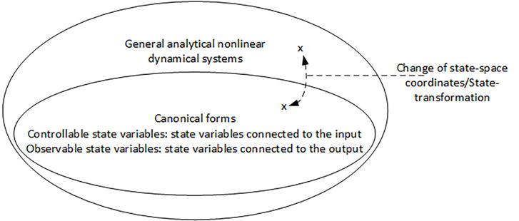
Figure 1.

Canonical forms facilitating simple definitions/explanations of controllability and observability as connectivities to the input and output representing structural properties of dynamical systems. Changes of coordinates/state-transformations connect general analytical nonlinear dynamical systems to their canonical forms.

Given the situation sketched in Figure 1, we asked ourselves the following question: “When considering nonlinear dynamical system structure, would it not be better to start from canonical representations”?

This chapter provides a positive answer by showing that canonical representations reveal structural properties easily and naturally. This allows us to define controllability and observability based on these connectivities. By first considering the structure of canonical forms, the mathematical complexity only comes in at the very end, when extending canonical representations to ordinary ones by means of state-transformations (see Figure 1). We will also show how these state-transformations and their associated Lie algebraic computations can be avoided completely by using sensitivity-based algorithms to establish controllability and observability. Avoiding these is especially important for large-scale systems. The algorithms compute a sensitivity rank condition (SERC) and uncontrollable/unobservable state-variables or modes, if any [17, 18, 19].

Remarkably, a canonical representation related to controllability/observability singularities, being points in the state-space where controllability/observability properties change, seems not to have been considered in the literature. A canonical form of controllability/observability singularities will be presented here and shown to be the key to considering nonlinear system structure as a global property, instead of a local one.

The terminology used in this chapter coincides with that commonly used in nonlinear system theory with one notable exception. What comes out as controllability in this chapter, is commonly known as local strong accessibility if the system is nonlinear and affine in the input [9, 10, 18, 19, 20]. We reflect on this notable exception and other results of this chapter in the conclusion section.

2. State-space representation of dynamical systems

To facilitate their analysis, numerical solution and control, dynamical systems described by ordinary differential equations are often represented in the so-called state-space form given by

$$\dot{x}\left(t\right)=f\left(x\left(t\right),u\left(t\right)\right),x\in {\mathbb{R}}^{n_x},u\in {\mathbb{R}}^{n_u},$$E1

$$y\left(t\right)=h\left(x\left(t\right)\right),y\in {\mathbb{R}}^{n_y}.$$E2

Within this formulation $t$ denotes time, $x\in {\mathbb{R}}^{n_x}$ is the state-vector or state collecting all state-variables $x_i,$ $i=1,2,\mathrm{..},n_x$, $u\in {\mathbb{R}}^{n_u}$ is the input-vector or input collecting all input-variables $u_i\in \mathbb{R},$ $i=1,2,\mathrm{..},n_u$, and $y\in {\mathbb{R}}^{n_y}$ is the output-vector or output collecting all output-variables $y_i,$ $i=1,2,\mathrm{..},n_y$. For convenience, we will generally drop the argument $t$. Eq. (1) describes how the state $x$ propagates and depends on the input $u$ and is called the state-equation. Eq. (2) describes how the state $x$ maps on the output $y$ and is called the output-equation. Several results from nonlinear system theory, used in this chapter, rely on differential geometry that applies to systems Eqs. (1) and (2) that are affine in the input, i.e.

$$f\left(x,u\right)=f_0\left(x\right)+\sum _{k=1}^{n_u}{f}_k\left(x\right)u_k,f_k\left(x\right)\in {\mathbb{R}}^{n_x},k=0,1,\mathrm{..},n_u.$$E3

In Eq. (3), $f_k\left(x\right)$,$k=0,1,\mathrm{..},n_u$, are vector functions with $f_0\left(x\right)$ called the drift term. Throughout this chapter $f$, $h$ in (1)–(3) are assumed to be analytic vector functions.

3. Canonical state-space representations of dynamical systems

3.1 Controllability as obtained from its canonical form

Reconsider Figure 1 and let

$$x^{\prime }=\mathrm{\Psi }\left(x\right),x^{\prime },x,\mathrm{\Psi }\in {\mathbb{R}}^{n_x}$$E4

represent the state-transformation that locally puts the system (1) into what will be called the controllability canonical form in this chapter, in line with the early development for linear systems as presented in [21], while appearing in [9, 10, 11] under different names associated with controllability.

$${\dot{x}}^{\prime }=f^{\prime }\left(x^{\prime },u\right),x^{\prime }=\left[\begin{array}{c}{x^{\prime }}^u\\ {x^{\prime }}^{\overline{u}}\end{array}\right]=\left[\begin{array}{c}{\mathrm{\Psi }}^u\left(x\right)\\ {\mathrm{\Psi }}^{\overline{u}}\left(x\right)\end{array}\right],f^{\prime }\left(x^{\prime },u\right)=\left[\begin{array}{c}{f^{\prime }}^u\left({x^{\prime }}^u,{x^{\prime }}^{\overline{u}},u\right)\\ {f^{\prime }}^{\overline{u}}\left({x^{\prime }}^{\overline{u}}\right)\end{array}\right].$$E5

In Eq. (5), the transformed state $x^{\prime }$ separates into ${x^{\prime }}^u$ containing state-variables that are connected and ${x^{\prime }}^{\overline{u}}$ containing state-variables that are disconnected from the input. A corresponding separation of the state-transformation $\mathrm{\Psi }\left(x\right)$ into ${\mathrm{\Psi }}^u\left(x\right)$ and ${\mathrm{\Psi }}^{\overline{u}}\left(x\right)$ is specified in (5). Each ${\mathrm{\Psi }}_i\left(x\right)$, $i=1,2,\mathrm{..},n_x$ is a scalar function of the state-variables $x$ and equal to the transformed state-variable $x_i^{\prime }$. Obviously, parts of the system denoted by the uppercase $\overline{u}$ that are disconnected from the input cannot be controlled.

Definition 1.

In the controllability canonical form (5), if $x_i^{\prime }\in {x^{\prime }}^{\overline{u}}$ then $x_i^{\prime }$ is called an uncontrollable state-variable of system (5) and ${\mathrm{\Psi }}_i\left(x\right)\in {\mathrm{\Psi }}^{\overline{u}}\left(x\right)$ is called an uncontrollable mode of system (1), (3). If $x_i^{\prime }\in {x^{\prime }}^u$, then $x_i^{\prime }$ is called a controllable state-variable of system (5) and ${\mathrm{\Psi }}_i\left(x\right)\in {\mathrm{\Psi }}^u\left(x\right)$ is called a controllable mode of system (1). ${\mathrm{\Psi }}_i\left(x\right)$ not necessarily depends on all state-variables $x_i$, $i=1,2,\mathrm{..},n_x$. The state-variables of the set $\left\{\left.x_i\right|{\mathrm{\Psi }}_i\left(x\right)\text{depends}\mathrm{on}{x}_i\right\}$ are called state-variables making up the controllable/uncontrollable mode ${\mathrm{\Psi }}_i\left(x\right)$.

Theorem 1.

1) Along trajectories of analytical systems (1), (3) the number of controllable modes $n_x^u=dim\left({\mathrm{\Psi }}^u\left(x\right)\right)$ and the number of uncontrollable modes $n_x^{\overline{u}}=dim\left({\mathrm{\Psi }}^{\overline{u}}\left(x\right)\right)$ is constant but may depend on the initial state. For most initial states, $n_x^u$, $n_x^{\overline{u}}$ are identical. For exceptional initial states, called singularities in Section 4, $n_x^u=n_x-n_x^{\overline{u}}$ is reduced. 2) Along trajectories of system (1), (3) the set of state-variables $\left\{\left.x_i\right|{\mathrm{\Psi }}^{\overline{u}}\left(x\right)\text{depends}\mathrm{on}{x}_i\right\}$ making up all uncontrollable modes is invariant.

Proof.

1) and 2) follow from the Hermann-Nagano theorem in [22] according to which the state-space of an analytical dynamical system (1), (3) foliates into manifolds of dimension $n_x^u$, as specified in Theorem 1. Trajectories of system (1), (3) stay on a single manifold, the manifold being determined by the initial condition. These manifolds can be described locally using the coordinates $x^{\prime }=\mathrm{\Psi }\left(x\right)$ given by state-transformation (4) into the controllability canonical form.

Corollary 1.

Within the controllability canonical form (5), uncontrollable state-variables ${x^{\prime }}^{\overline{u}}$ and controllable state-variables ${x^{\prime }}^u$ correspond one-to-one with uncontrollable modes ${\mathrm{\Psi }}^{\overline{u}}\left(x\right)$ and controllable modes ${\mathrm{\Psi }}^u\left(x\right)$ of the system (1). The uncontrollable state-variables and modes are disconnected from the input, whereas the controllable state-variables and modes are connected to the input. Along trajectories of analytical systems (1), (3) the number of controllable and uncontrollable modes $n_x^u,n_x^{\overline{u}}$ are invariant but may depend on the initial state of the trajectory. For most initial states, $n_x^u,n_x^{\overline{u}}$ have the same value. For exceptional initial states, called controllability singularities in Section 4, the number of controllable modes $n_x^u=n_x-n_x^{\overline{u}}$ is reduced. Along trajectories of analytical systems (1), (3) the set of state-variables making up all uncontrollable modes is invariant.

Definition 1 together with Corollary 1 are graphically represented by Figure 2. From them the following alternative definition of controllability in terms of connectivities is obtained.

Figure 2.

Graphical representation and partitioning of a system with an input $u$ along a trajectory. The state-space naturally partitions into a controllable part represented by the controllable modes ${\mathrm{\Psi }}^u\left(x\right)$ and an uncontrollable part represented by the uncontrollable modes ${\mathrm{\Psi }}^{\overline{u}}\left(x\right)$. ${\mathrm{\Psi }}^{\overline{u}}\left(x\right)$ is disconnected from the input whereas ${\mathrm{\Psi }}^u\left(x\right)$ is connected to the input. Connections internal to the system are represented by arrows with broken lines.

Definition 2.

Analytical dynamical systems (1), (3) are controllable along a trajectory if in the controllability canonical form (5) no state-variable $x_i^{\prime }$, $i=1,2,\mathrm{..},n_x$, or equivalently no mode ${\mathrm{\Psi }}_i\left(x\right)$ of system (1), (3), is disconnected from the input.

Remark 1.

Computation of the state-transformation $\mathrm{\Psi }\left(x\right)$ is generally performed using Lie algebraic computations [9, 10, 11]. These generally become problematic and time-consuming for large-scale systems. Sensitivity-based algorithms, especially developed for large-scale systems, provide a very attractive alternative [17, 18, 19]. In Section 5 we will elaborate on this.

Theorem 2.

Without having to compute the state-transformation (4), sensitivity-based algorithms very efficiently compute $n_x^u=dim\left({x^{\prime }}^u\right)$ and $n_x^{\overline{u}}=dim\left({x^{\prime }}^{\overline{u}}\right)$ as well as the set of state-variables making up all uncontrollable modes ${x^{\prime }}^{\overline{u}}$ within the controllability canonical form (5), along trajectories of analytical systems (1), (3).

Proof.

Follows from [18] in which $n_x^u=dim\left({x^{\prime }}^u\right)$, $n_x^{\overline{u}}=dim\left({x^{\prime }}^{\overline{u}}\right)$ and the set of state-variables making up all uncontrollable modes are all obtained from a singular value decomposition (SVD) of a sensitivity matrix $S\in {\mathbb{R}}^{n_r\times n_x},n_r\ge n_x$. Each zero singular value represents an uncontrollable mode, and each nonzero singular value a controllable mode. The nonzero components of the corresponding right singular vectors indicate the state-variables making up the corresponding mode.

3.2 Observability as obtained from its canonical form

A development very similar to that of controllability in the previous section applies to observability. Because of this similarity, this section focuses on the differences. Reconsider Figure 1 and let

$$x^{\prime }=\mathrm{\Psi }\left(x\right),x^{\prime },x,\mathrm{\Psi }\in {\mathbb{R}}^{n_x}$$E6

now represent the state-transformation that locally puts the system (1)–(3) into what will be called the observability canonical form in this chapter while appearing in [9, 10, 11] under different names associated with observability.

$$\begin{array}{l}{\dot{x}}^{\prime }=f\left(x^{\prime },u\right),y^{\prime }=h\left(x^{\prime }\right),\\ x^{\prime }=\left[\begin{array}{c}{x^{\prime }}^y\\ {x^{\prime }}^{\overline{y}}\end{array}\right]=\left[\begin{array}{c}{\mathrm{\Psi }}^y\left(x\right)\\ {\mathrm{\Psi }}^{\overline{y}}\left(x\right)\end{array}\right],f\left(x^{\prime },u\right)=\left[\begin{array}{c}{f}^y\left({x^{\prime }}^y,u\right)\\ f^{\overline{y}}\left({x^{\prime }}^y,{x^{\prime }}^{\overline{y}},u\right)\end{array}\right],h\left(x^{\prime }\right)=h\left({x^{\prime }}^y\right)\end{array}$$E7

In Eq. (7), the state $x^{\prime }$ separates into ${x^{\prime }}^y$ containing state-variables that are connected and ${x^{\prime }}^{\overline{y}}$ containing state-variables that are disconnected from the output. A corresponding separation of the state-transformation $\mathrm{\Psi }\left(x\right)$ into ${\mathrm{\Psi }}^y\left(x\right)$ and ${\mathrm{\Psi }}^{\overline{y}}\left(x\right)$ is specified in (7). Given the similarities with controllability in the previous section Definition 1, Theorem 1, Definition 2, Corollary 1 and Theorem 2 in the previous section apply if controllability is replaced by observability, Eq. (5) by (7) and input $u$ by output $y$. Figure 2 then turns into Figure 3.

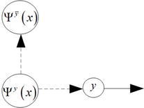
Figure 3.

Graphical representation and partitioning of a system with an output $y$ along a trajectory. The state-space naturally partitions into an observable part represented by the observable modes ${\mathrm{\Psi }}^y\left(x\right)$ and an unobservable part represented by the unobservable modes ${\mathrm{\Psi }}^{\overline{y}}\left(x\right)$. ${\mathrm{\Psi }}^{\overline{y}}\left(x\right)$ is disconnected from the output whereas ${\mathrm{\Psi }}^y\left(x\right)$ is connected to the output. Connections internal to the system are represented by arrows with broken lines.

Remark 2.

To construct analytical systems having certain controllability/observability properties, one can select the corresponding canonical form and choose the system parts arbitrarily. This generically realizes the corresponding controllability/observability properties, since there is the possibility, having zero probability, that an arbitrary choice causes additional uncontrollable/unobservable modes. Having realized the appropriate controllability/observability properties this way, we may subsequently “hide” them the by performing a state-transformation.

Remark 3.

Following Remark 2, all canonical forms have the property that the system parts do not cause additional uncontrollable/unobservable modes.

3.3 The Kalman canonical form of analytical nonlinear dynamical systems

Partitioning of systems along trajectories into parts that do and do not connect to the system input and output were obtained in sections 3.1, 3.2. These parts are represented by controllable/uncontrollable and observable/unobservable modes. These two separations lead naturally to a separation into four system parts, as represented for linear systems by the Kalman decomposition [3]. A similar decomposition for nonlinear system exists [9, 10, 11]. As before, the latter decomposition is obtained from a suitable state-transformation

$$x^{\prime }=\mathrm{\Psi }\left(x\right),x^{\prime },x,\mathrm{\Psi }\in {\mathbb{R}}^{n_x}$$E8

that now transforms the system into the form

$$\begin{array}{l}{\dot{x}}^{\prime }=f^{\prime }\left(x^{\prime },u\right),x^{\prime }=\left[\begin{array}{c}{x^{\prime }}^{u\overline{y}}\\ {x^{\prime }}^{uy}\\ {x^{\prime }}^{\overline{u}\overline{y}}\\ {x^{\prime }}^{\overline{u}y}\end{array}\right]=\left[\begin{array}{c}{\mathrm{\Psi }}^{u\overline{y}}\left(x\right)\\ {\mathrm{\Psi }}^{\mathit{uy}}\left(x\right)\\ {\mathrm{\Psi }}^{\overline{u}\overline{y}}\left(x\right)\\ {\mathrm{\Psi }}^{\overline{u}y}\left(x\right)\end{array}\right],f^{\prime }\left(x,u\right)=\left[\begin{array}{c}{f^{\prime }}^{u\overline{y}}\left({x^{\prime }}^{u\overline{y}},{x^{\prime }}^{uy},{x^{\prime }}^{\overline{u}\overline{y}},{x^{\prime }}^{\overline{u}y},u\right)\\ {f^{\prime }}^{uy}\left({x^{\prime }}^{uy},{x^{\prime }}^{\overline{u}y},u\right)\\ {f^{\prime }}^{\overline{u}\overline{y}}\left({x^{\prime }}^{\overline{u}y},x^{\overline{u}\overline{y}}\right)\\ {f^{\prime }}^{\overline{u}y}\left({x^{\prime }}^{\overline{u}y}\right)\end{array}\right],\\ y^{\prime }=h^{\prime }\left(x\right)=h^{\prime }\left({x^{\prime }}^{uy},{x^{\prime }}^{\overline{u}y}\right)\end{array}$$E9

where ${\mathrm{\Psi }}^{u\overline{y}}\left(x\right)$ are controllable and unobservable modes that are connected to the input and disconnected from the output and similarly for ${\mathrm{\Psi }}^{\mathit{uy}}\left(x\right),{\mathrm{\Psi }}^{\overline{u}\overline{y}}\left(x\right)$ and ${\mathrm{\Psi }}^{\overline{u}y}\left(x\right)$. The decomposition (9) will be called the controllability observability canonical form or Kalman canonical form in this chapter. It is graphically represented by Figure 4.

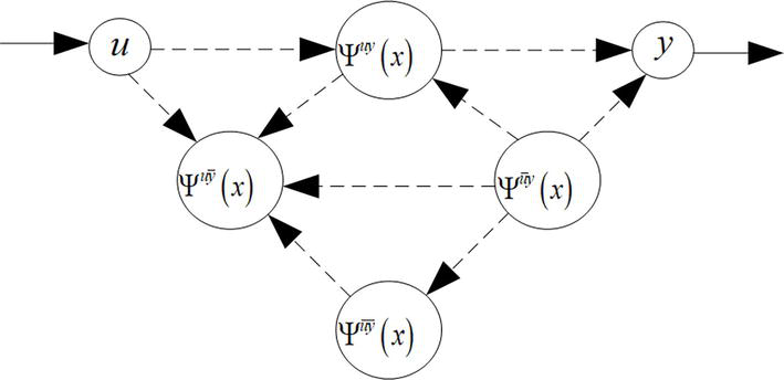
Figure 4.

Graphical representation and partitioning of a system with input $u\in {\mathbb{R}}^{n_u}$ and output $y\in {\mathbb{R}}^{n_y}$along a trajectory. The state-space partitions into four parts represented by the modes ${\mathrm{\Psi }}^{u\overline{y}}\left(x\right)$, ${\mathrm{\Psi }}^{\mathit{uy}}\left(x\right),{\mathrm{\Psi }}^{\overline{u}\overline{y}}\left(x\right)$ and ${\mathrm{\Psi }}^{\overline{u}y}\left(x\right)$. The partitioning is based on whether or not system parts connect to the input and output.

Remark 4.

Not all system parts in Figures 2-4 have to be present. Also, not all internal connections have to be present as long as the connectivity of system parts with the system input and output remains unchanged. In Figure 4 for example, the connection from ${\mathrm{\Psi }}^{\mathit{uy}}\left(x\right)$ to ${\mathrm{\Psi }}^{u\overline{y}}\left(x\right)$ may be absent as well as the one from ${\mathrm{\Psi }}^{\overline{u}y}\left(x\right)$ to ${\mathrm{\Psi }}^{\overline{u}\overline{y}}\left(x\right)$.

Remark 5.

From Figure 4 observe that ${\mathrm{\Psi }}^{\mathit{uy}}\left(x\right)$ in the only part that may be controlled by output feedback.

4. Controllability/observability singularities: Initial states affecting nonlinear system structure

Linear systems are described by (1)–(3) with

$$f\left(x,u\right)=\mathit{Fx}+\mathit{Gu},h\left(x\right)=\mathit{Hx}.$$E10

$F,G$ and $H$ are real matrices that fully determine the interconnections and system structure. The entries of $F,G$ and $H$ do not depend on $x$ nor on $u$. Therefore, the time-dependency of the state $x$ and input $u$ does not change the system structure [3].

For analytical nonlinear dynamical systems (1)–(3) however, this need no longer be the case. Initial states may switch-off, i.e. disconnect, connections to the input and output, thereby changing the system structure [16, 23]. To illustrate this, we start with an example presented in the next section.

4.1 Examples and definition of controllability/observability singularities

Example 1

$$\dot{x}=f\left(x,u\right),f\left(x,u\right)=\left[\begin{array}{c}-2x_1-x_3+u_1\\ \left(1-x_2\right)\left(x_1+u_1\right)\\ -x_1\end{array}\right],x,f\in {\mathbb{R}}^3,u\in {\mathbb{R}}^1,$$E11

$$y=h\left(x\right),h\left(x\right)=\left[\begin{array}{c}\left(1-x_2\right)x_3\\ x_2\end{array}\right],y,h\in {\mathbb{R}}^2.$$E12

If, in Eq. (11), we take $x_2\left(0\right)=1$, then ${\dot{x}}_2=0$ and thus $x_2=1$ over the entire time-domain. In this way, the constant state-variable $x_2$ disconnects itself from the other state-variables and input. From the output-Eq. (12) and $x_2\equiv 1$, we observe that both $x_3$ and $x_1$ are disconnected from the output. These disconnections reduce the number of controllable state-variables connected to the input as well as the number of observable state-variables connected to the output. Accordingly, the system structure is changed. Application of a state-transformation to system (11), (12) and initial states satisfying $x_2\left(0\right)=1$, does not change the system structure, but does change state-variables into modes and constant state-variables into non-constant ones. To stress the role of initial conditions in determining system structure [23], we introduce the following definition.

Definition 3.

Initial states of the analytical dynamical system (1)–(3) that reduce the number of controllable/observable modes as compared to initial states in their neighborhood we call controllability/observability singularities of the analytic system (1)–(3).

Controllability singularities occur for instance in chemical systems when zero initial concentrations of some species prevent subsequent chemical reactions to occur [15]. They are different from what are mostly called singular states of dynamical systems which have a different degree of non-holonomy as compared to neighboring states [24]. As to our Example 1, according to Definition 3, initial states satisfying $x_2\left(0\right)=1$ are both controllability as well as observability singularities of system (11), (12).

In Example 1, if $x_2=1$ would hold at isolated times only, this does not affect system structure since the disconnections from the input and output disappear immediately. But if $x_2=1$ holds along some part of a trajectory, the system structure changes along that part of the trajectory causing what is called temporal system structure [25, 26, 27]. Because analytical dynamical systems do not allow state-variables to be constant on a time-interval and time-varying outside this time-interval, the structure of analytic systems is fixed along trajectories [22]. But analytic systems do allow state-variables to be very close to being constant along part of a trajectory. In Example 1, when $x_2$ becomes very close to $1$, one may say that the analytic system (11), (12) “almost changes structure” [27]. But for $x_2$ to really change the analytic system structure, it needs to be exactly $1$ over the entire time domain. For arbitrary inputs $u\left(t\right)$ this can only happen if state-variable $x_2=1$ is disconnected from the input and other state-variables, so when $x_2\left(0\right)=1$.

We deliberately constructed system (11), (12), starting from both the controllability canonical form (5) and the observability canonical form (7), while letting the constant state-variable $x_2=1$, that is disconnected from the other state-variables and input, switch-off state-variables from the input and output causing the controllability and observability singularities. The next theorem states that this type of switching is the basic mechanism causing controllability and observability singularities.

Theorem 3.

For analytical dynamical systems (1)–(3), canonical representations of controllability/observability singularities exist in which constant state-variables that are disconnected from the input and the remaining state-variables switch-off state-variables from the input/output causing the controllability/observability singularities.

The canonical representations of controllability/observability singularities will be given in the next section and the proof in Appendix 2. As to controllability, observe that Definition 3 and Theorem 3 comply with the Hermann-Nagano theorem [22], stating that for analytic systems (1)–(3) the number of uncontrollable modes $n_x^{\overline{u}}=dim\left(x^{\overline{u}}\right)$ is fixed along trajectories, but may depend on the initial state.

4.2 Canonical state-space representations of controllability/observability singularities

To obtain the canonical representation of controllability singularities, we start from the controllability canonical representation (5) dropping accents of transformed states. We denote by $x^{s\overline{u}}$ the state-vector containing the constant state-variables that realize the switching-off. The switching-off occurs if $x^{s\overline{u}}\left(0\right)={\overline{x}}^{s\overline{u}},$ in which ${\overline{x}}^{s\overline{u}}$ is a steady state of $x^{s\overline{u}}$ that is unaffected by the input and state-variables not contained in $x^{s\overline{u}}$. We denote by $x^{u\overline{u}}$ the vector of state-variables that become uncontrollable because they are switched-off from the input and by vector $x^{\mathit{uu}}$ the controllable state-variables that are not switched-off from the input, and so:

$$x^u=\left[\begin{array}{c}{x}^{\mathit{uu}}\\ x^{u\overline{u}}\end{array}\right].$$E13

To the controllability singularities $x^{s\overline{u}}\left(0\right)={\overline{x}}^{s\overline{u}}$ the following canonical singular controllability form corresponds:

$$\left[\begin{array}{c}{\dot{x}}^{\mathit{uu}}\\ {\dot{x}}^{u\overline{u}}\\ {\dot{x}}^{\overline{u}}\end{array}\right]=\left[\begin{array}{c}{f}^{\mathit{uu}}\left(x^{\mathit{uu}},x^{u\overline{u}},x^{\overline{u}},u\right)\\ f^{u\overline{u}}\left(x^{\mathit{uu}},x^{u\overline{u}},x^{\overline{u}},u\right)\\ f^{\overline{u}}\left(x^{\overline{u}}\right)\end{array}\right].$$E14

$$x^{s\overline{u}}\left(0\right)={\overline{x}}^{s\overline{u}}\Rightarrow x^{s\overline{u}}\left(t\right)={\overline{x}}^{s\overline{u}},f^{u\overline{u}}\left(x^{\mathit{uu}},x^{u\overline{u}},x^{\overline{u}},u\right)=f^{u\overline{u}}\left(x^{u\overline{u}},x^{\overline{u}}\right),-\infty <t<\infty .$$E15

Eq. (15) describes that if $x^{s\overline{u}}\left(0\right)={\overline{x}}^{s\overline{u}}$, $x^{s\overline{u}}$are constant state-variables, unaffected by the input and state-variables not captured by $x^{s\overline{u}}$, that realize the switching-off. Therefore,

$$x^{s\overline{u}}\supset \left\{x^{u\overline{u}},x^{\overline{u}}\right\}$$E16

In a similar fashion, starting from the observability canonical representation (7), observability singularities $x^{s\overline{y}}\left(0\right)={\overline{x}}^{s\overline{y}}$ switch-off state-variables from the output. We denote the vector of state-variables that become unobservable because they are switched-off from the output by $x^{y\overline{y}}.$Vector $x^{\mathit{yy}}$ represents the observable state-variables that are not switched-off from the output, and therefore:

$$x^y=\left[\begin{array}{c}{x}^{\mathit{yy}}\\ x^{y\overline{y}}\end{array}\right].$$E17

To the observability singularities $x^{s\overline{y}}\left(0\right)={\overline{x}}^{s\overline{y}}$ the following canonical singular observability form corresponds:

$$\dot{x}=\left[\begin{array}{c}{\dot{x}}^{\mathit{yy}}\\ {\dot{x}}^{y\overline{y}}\\ {\dot{x}}^{\overline{y}}\end{array}\right]=\left[\begin{array}{c}{f}^{\mathit{yy}}\left(x^{\mathit{yy}},x^{y\overline{y}}\right)\\ f^{y\overline{y}}\left(x^{\mathit{yy}},x^{y\overline{y}}\right)\\ f^{\overline{y}}\left(x^{\mathit{yy}},x^{y\overline{y}},x^{\overline{y}}\right)\end{array}\right],y=h\left(x^{\mathit{yy}},x^{y\overline{y}}\right).$$E18

$$x^{s\overline{y}}\left(0\right)={\overline{x}}^{s\overline{y}}\Rightarrow x^{s\overline{y}}\left(t\right)={\overline{x}}^{s\overline{y}},f^{\mathit{yy}}\left(x^{\mathit{yy}},x^{y\overline{y}}\right)=f^{\mathit{yy}}\left(x^{\mathit{yy}}\right),h\left(x^{\mathit{yy}},x^{y\overline{y}}\right)=h\left(x^{\mathit{yy}}\right),-\infty <t<\infty .$$E19

Eq. (19) describes that if $x^{s\overline{y}}\left(0\right)={\overline{x}}^{s\overline{y}}$, $x^{s\overline{y}}$ are constant state-variables, unaffected by the input and state-variables not captured by $x^{s\overline{y}}$, that realize the switching-off.

Theorem 4.

By considering controllability/observability singularities as different systems, the structural properties of analytical dynamical systems (1)–(3) become global.

Proof.

From Theorem 1, the number of controllable and observable modes is constant along any trajectory of an analytical dynamical system (1)–(3). Therefore, these only depend on the initial state of a trajectory. By Definition 3, controllability/observability singularities are the only ones changing system structure.

5. Determining system structure through sensitivity-based algorithms

5.1 Determining controllability/observability of systems and individual state-variables

Because uncontrollable state-variables and modes are disconnected from the input, their sensitivity to input-variables vanishes. Because unobservable state-variables and modes are disconnected from the output, the sensitivity of the output to them, vanishes. Sensitivity-based algorithms capture these insights by calculating a sensitivity matrix $S\in {\mathbb{R}}^{n_r\times n_x},n_r\ge n_x$ [17, 18, 19] along a trajectory of system (1)–(3). As stated by Theorem 2, a singular value decomposition (SVD) of this matrix provides the number of uncontrollable/unobservable modes as the number of zero singular values. In other words, if the matrix is full-rank i.e. having no zero singular values, the system is controllable/observable along the trajectory and satisfies what is called a sensitivity rank condition (SERC) in [17, 18, 19]. Moreover, the state-variables making up each controllable/observable and uncontrollable/unobservable mode are indicated by the nonzero components of the corresponding right singular vectors. The state-variables making up the uncontrollable/unobservable modes are represented by what is called a controllability/observability signature in [17, 18, 19]. Thereby, without calculating state-transformations and canonical forms, the sensitivity-based algorithm provides almost all information system and control engineers are interested in. Specifically, they determine the controllability and observability of individual state-variables of the system (1)–(3) when applying the following definition.

Definition 4.

A state-variable $x_i$, $i=1,2,\mathrm{..},n_x$ is called controllable/observable if it does not make up any uncontrollable/unobservable mode. Otherwise, state-variable $x_i$ is called uncontrollable/unobservable.

5.2 A challenging small-scale example containing two controllability singularities

Although being small-scale, the example presented next is a challenging one, because it contains two controllability singularities. Also, close to the singularity, transformed state-variables that have to be computed by the sensitivity-based algorithm, tend to grow very large. The example illustrates the Hermann-Nagano theorem in [22], which is used and described in the proof of Theorem 1, as well as the canonical form of controllability singularities.

Example 2: An uncontrollable system with two controllability singularities.

$$\dot{x}=f\left(x,u\right)=\left[\begin{array}{c}-x_2\\ x_1\\ 0\end{array}\right]u_1+\left[\begin{array}{c}2x_3{x}_1\\ 2x_3{x}_2\\ x_3^2+1-x_1^2-x_2^2\end{array}\right]u_2$$E20

System (20) originates from [11], example 3.8. From the analysis of this example in [11], we conclude that system (20) has a single uncontrollable mode foliating the state-space into submanifolds with dimension 2. These submanifolds are tori given by the equation

$$\left(x_1^2+x_2^2+x_3^2+1\right)/\sqrt{x_1^2+x_2^2}=c,$$E21

with $c>2$ a constant that is determined by the initial conditions. This constant tends to infinity when approaching the singularity $x_1=x_2=0$, where the torus degenerates into the $x_3$ axis. The other singularity occurs for $x_1^2+x_2^2=1$, $x_3=0$, resulting in $c=2$, where the torus degenerates into a circle (Appendix 1 provides further details). The dimensions of this foliation are thus two for the tori and one for the $x_3$ axis and circle $x_1^2+x_2^2=1,$ $x_3=0$.

Figure 5 concerns the controllability of system (20). It graphically represents the singular values ${\sigma }_i,i=1,2,3$ (left panel) determining SERC and the components of the right singular vector ${\nu }_3$(right panel) corresponding to the only (numerically) zero singular value ${\sigma }_3$ making up the controllability signature [18]. From the right panel of Figure 5, we observe that all the components of ${\nu }_3$ are nonzero, implying that all three state-variables together make up the single uncontrollable mode. Therefore, according to Definition 4, no state-variable is controllable. When represented in the controllability canonical form (5), obtained after state-transformation (22), to be presented in the next section, the single uncontrollable mode is transformed into the single uncontrollable state-variable $x_3^{\prime }=1/c$. This is confirmed by the controllability signature in the right panel of Figure 6. Then, according to Definition 4, the other two state-variables $x_1^{\prime }=x_3$, $x_2^{\prime }=x_1$ are controllable.

Figure 5.

Singular values (left panel) and controllability signature (right panel) of system (20) confirming the existence of one uncontrollable mode involving all three state-variables.

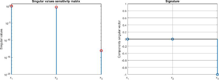
Figure 6.

Singular values and controllability signature after transformation (22) into the controllability canonical form (5) showing $x_3^{\prime }=1/c$ as the only uncontrollable mode and state-variable.

Figure 7 shows directed graphs of the original system (20) (left panel) and its controllability canonical form (right panel). Observe that only the latter directed graph reveals uncontrollability, illustrating that directed graphs only reveal uncontrollability/unobservability, when the system is represented in canonical form (minus permutations of state-variables).

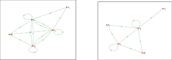
Figure 7.

Directed graph of system (20) (left panel) and its controllability canonical form (right panel). Only the latter reveals uncontrollability of state-variable $x_3^{\prime }=1/c$.

In the next section we will show how each of the two controllability singularities can be made to match the canonical singular controllability form (14), (15). Note that this canonical form is obtained as a special case of the controllability canonical form (5). The latter canonical form will therefore also be obtained in the next section.

5.2.1 Canonical representations of the two controllability singularities

For system (20), the controllability singularity $x_1\left(0\right)=x_2\left(0\right)=0$, implies $x_1\left(t\right)=x_2\left(t\right)=0$, $t\ge 0$, which gives rise to two uncontrollable modes involving state-variables $x_1$ and $x_2$. This leaves state-variable $x_3$ as the single controllable state-variable, as confirmed by Figure 8.

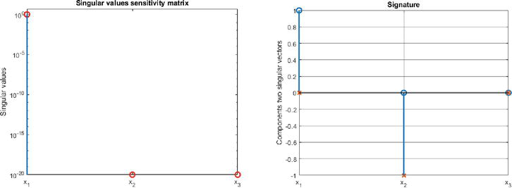
Figure 8.

Singular values (left panel) and controllability signature (right panel) of the controllability singularity $x_1\left(0\right)=x_2\left(0\right)=0$ of system (20). These confirm two uncontrollable modes involving state-variables $x_1$ and $x_2$, leaving one controllable state-variable $x_3$ .

Since $x_3$ is the single controllable state-variable, in the canonical singular controllability representation (14), (15) $x^{\mathit{uu}}$ can only involve state-variable $x_3$ and we take $x^{\mathit{uu}}=x_3$. Since $c$ in Eq. (21) is constant it may serve as $x^{\overline{u}}$. However, $c\to \infty$ as $x_1\to 0$, $x_2\to 0$. This is overcome by taking $x^{\overline{u}}=1/c$. Finally, we may choose either $x_1$ or $x_2$ as $x^{u\overline{u}}$. For $x^{u\overline{u}}=x_1$, the state-transformation into the canonical singular controllability form (14) becomes

$$x^{\prime }=\left[\begin{array}{c}{x}_1^{\prime }\\ x_2^{\prime }\\ x_3^{\prime }\end{array}\right]=\left[\begin{array}{c}{x^{\prime }}^{\mathit{uu}}\\ {x^{\prime }}^{u\overline{u}}\\ {x^{\prime }}^{\overline{u}}\end{array}\right]=\left[\begin{array}{c}{x}_3\\ x_1\\ 1/c\end{array}\right]=\mathrm{\Psi }\left(x\right),$$E22

with ${x^{\prime }}^{s\overline{u}}={\left[x_2^{\prime },x_3^{\prime }\right]}^T={\left[x_1,1/c\right]}^T$ and ${\overline{x^{\prime }}}^{s\overline{u}}={\left[0,0\right]}^T$. Appendix 1 reveals that the inverse $x={\mathrm{\Psi }}^{-1}\left(x^{\prime }\right)$ is only one-to-one locally. Figure 9 confirms that $x_1^{\prime }=x_3$ is the single controllable mode and state-variable. The two uncontrollable modes involve the other two state-variables $x_2^{\prime }=x_1=0$, $x_3^{\prime }=1/c=0$, $-\infty <t<\infty$.

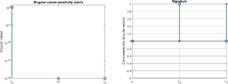
Figure 9.

Singular values and controllability signature after transformation (22) into the canonical singular controllability form (14) showing $x_1^{\prime }=x_3$ as the only controllable mode and state-variable.

The second controllability singularity of system (20) concerns initial states satisfying $x_1^2\left(0\right)+x_2^2\left(0\right)=1$, $x_3\left(0\right)=0$. Then $x_1^2\left(t\right)+x_2^2\left(t\right)=1$, $x_3\left(t\right)=0$, $-\infty <t<\infty$ and the torus (21) degenerates into a circle which is obtained for $c=2$. Figure 10 confirms that we obtain the canonical singular controllability form (14), (15) by taking ${x^{\prime }}^{\mathit{uu}}=x_1$, ${x^{\prime }}^{u\overline{u}}=x_3$, ${x^{\prime }}^{\overline{u}}=1/c$, ${x^{\prime }}^{\mathit{su}}={\left[x_2^{\prime },x_3^{\prime }\right]}^T$ and ${\overline{x^{\prime }}}^{\mathit{su}}={\left[0,1/2\right]}^T$, i.e. by means of the state-transformation

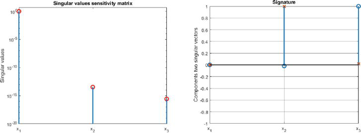
Figure 10.

Singular values and signature after transformation (23) into the canonical singular controllability form (14) showing $x_1^{\prime }=x_1$ as the only controllable mode and state-variable.

$$x^{\prime }=\left[\begin{array}{c}{x}_1^{\prime }\\ x_2^{\prime }\\ x_3^{\prime }\end{array}\right]=\left[\begin{array}{c}{x^{\prime }}^{\mathit{uu}}\\ {x^{\prime }}^{u\overline{u}}\\ {x^{\prime }}^{\overline{u}}\end{array}\right]=\left[\begin{array}{c}{x}_1\\ x_3\\ 1/c\end{array}\right]=\mathrm{\Psi }\left(x\right).$$E23

As a second example we reconsider system (11), (12) of Example 1. From our sensitivity-based algorithm we find system (11) to be controllable, since the singular values obtained are $3.2782\mathrm{e}+00$, $7.5852\mathrm{e}-01$ and $2.6537\mathrm{e}-02$. This system has a controllability singularity $x_2\left(0\right)=1$. Figure 11 displays the singular values and controllability signature of this canonical controllability singularity, showing that only the 2nd component is nonzero confirming that $x_2$ is the only uncontrollable state-variable. From our sensitivity-based algorithm we also find system (11), (12) to be observable, since the singular values obtained are $2.0052\mathrm{e}+00$, $8.5798\mathrm{e}-01$ and $3.4738\mathrm{e}-01$. As explained in Section 4.1 $x_2\left(0\right)=1$ is also an observability singularity. Figure 12 confirms this, showing that $x_2$ is the only state-variable that remains observable.

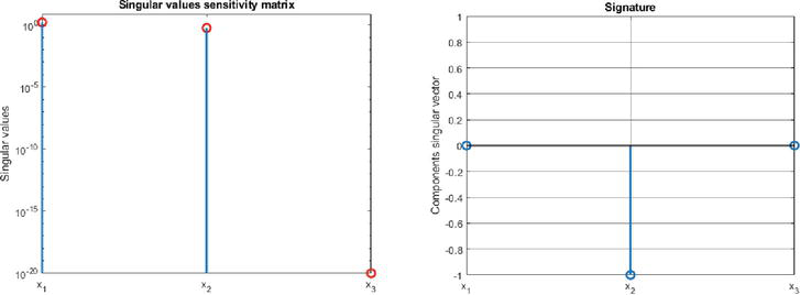
Figure 11.

Singular values (left panel) and controllability signature (right panel) of the controllability singularity $x_2\left(0\right)=1$ of system (11).

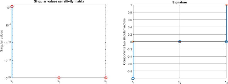
Figure 12.

Singular values (left panel) and observability signature (right panel) of the observability singularity $x_2\left(0\right)=1$ of system (11), (12).

To summarize, for system (11), (12) of Example 1, $x^{s\overline{u}}\left(0\right)=x_2\left(0\right)=1={\overline{x}}^{s\overline{u}}$ is a canonical controllability singularity satisfying (14) with $x^u=x_1$, $x^{u\overline{u}}={\left[x_2,x_3\right]}^T$ and $x^{\overline{u}}=\varnothing ,$ as well as a observability canonical singularity $x^{s\overline{y}}\left(0\right)=x_2\left(0\right)=1={\overline{x}}^{s\overline{y}}$ satisfying (17) with $x^y=x_2,x^{y\overline{y}}={\left[x_1,x_3\right]}^T$and $x^{\overline{y}}=\varnothing$.

5.3 Large-scale examples

To illustrate and challenge the capability of sensitivity-based algorithms to solve high-dimensional problems efficiently, we generated large-scale nonlinear dynamical systems having 200 state-variables and 25 input-variables, following Remark 2 at the end of Section 3.3. Within the controllability canonical form of linear systems [3, 21], we selected the nonzero parts of the time-invariant system matrices random, while taking different values for the number of uncontrollable state-variables: $n_x^{\overline{u}}=0,1,2,\mathrm{..},20$. To change these linear time-invariant systems into nonlinear systems with $n_x^{\overline{u}}$ uncontrollable modes, we applied the following nonlinear state-transformation

$$x_i^{\prime }=x_i,x_{i+1}^{\prime }=e^{x_i+x_{i+1}},i=1,3,5,7,\mathrm{..},199.$$E24

We applied the sensitivity-based algorithm to the nonlinear systems with state $x^{\prime }$. The left panel of Figure 13 shows the singular values obtained from the sensitivity-based algorithm.

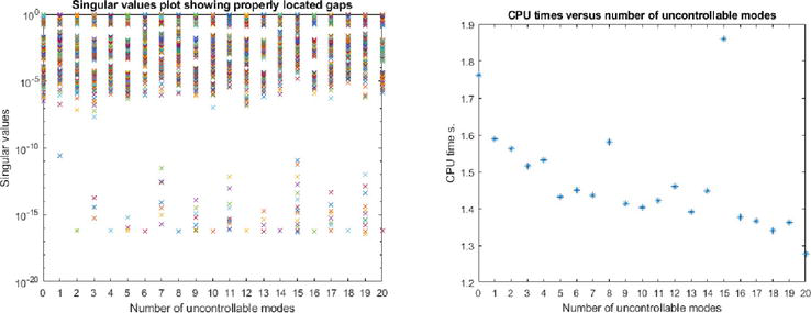
Figure 13.

The sensitivity-based algorithm correctly (left panel) and efficiently (right panel) establishes the number of uncontrollable modes of systems with 200 state-variables and 25 input-variables: The number of uncontrollable modes in each case equals the number of numerically zero singular values because some of these overlaps.

It shows that all gaps in the singular values are properly located (recognizing that several singular values overlap), because the number of singular values below this gap should be considered numerically zero, each one corresponding to an uncontrollable mode. The right panel shows the very short CPU times required to compute each result that is based on the concatenation of sensitivity matrices of three short trajectories. For details concerning the sensitivity-based algorithm we refer to [17, 18, 28]. We only mention here that, by exploiting duality, the sensitivity-based algorithm is also able to establish observability of nonlinear systems. The computations we performed on an ordinary PC using MATLAB.

6. Conclusions

We showed how canonical representations and sensitivity-based algorithms simplify and unify the definition, analysis and computation of controllability and observability of analytical, nonlinear and dynamical systems. For dynamical systems represented in canonical form, controllability/observability simply translate into whether state-variables connect to the input/output. For systems not represented by canonical forms, we showed that controllability/observability translates into scalar functions of all state-variables, called modes, being connected to the input/output. Controllable/observable and uncontrollable/unobservable modes, as well as the state-variables involved in these modes, we computed very efficiently, using sensitivity-based algorithms. These algorithms nicely circumvent Lie algebraic computations, as well as state-transformations into canonical forms, which may both give rise to computational difficulties, especially for large-scale systems.

As for the restriction in this chapter to only study analytical dynamical systems, we remark that systems not belonging to this class are usually piecewise analytic. Then the analysis and results of this chapter apply to each separate interval over which the system is analytic. We also remark that by augmenting the system state with constant parameters, we can include the structural property identifiability as a special case of observability.

Originally, controllability is the ability to steer the system from any state to another, by means of the input. According to the analysis and definitions presented here, controllability relates to the connectivity of internal state-variables and modes to the input. For linear systems they are equivalent. If the system is nonlinear and affine in the input, our definition of controllability corresponds to what in the literature is usually called local strong accessibility, that is a slightly weaker property if the drift term is nonzero. As for the observability of dynamical systems, no such subtle difference occurs.

Starting from conventional canonical forms, we constructed new canonical forms of structural singularities, obtained from the insight that these are caused by initial conditions that permanently switch-off connections to the input/output. This insight also suggests to consider structural singularities as different systems. We showed how this turns system structure, determined by the dimensions of subsystems within corresponding canonical forms, into a global property. On the other hand, state-transformations into canonical forms may hold only locally.

If the state-space model has been developed from first principles (e.g. energy conservation, Newton’s laws), state-variables have a clear meaning and interpretation. Since sensitivity-based algorithms provide the state-variables involved in the uncontrollable and unobservable modes, they then immediately provide the exact information a system modeler, designer or engineer is interested in.

Acknowledgments

The author likes to thank Hans Stigter, Jaap Molenaar, Dominique Joubert and Andrew Laidlaw for providing valuable ideas, discussions and suggestions that improved, and partly inspired, this chapter.

Declarations

The author has no conflicts of interest to disclose.

The author has no relevant financial or non-financial interests to disclose.

Data will be made available on reasonable request.

.

A. Appendix 1. Example 2 and the local character of its state-transformations.

The state-space of system (20) in Example 2, according to [11] example 3.8, is foliated as represented by Figure 14.

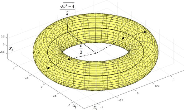
Figure 14.

The manifolds of example 2 are tori described by $\left(x_1^2+x_2^2+x_3^2+1\right)/\sqrt{x_1^2+x_2^2}=c>2$ with $c$ a constant. The two singularities are the circle $c=2$,$x_1^2+x_2^2=1$,$x_3=0$ and the $x_3$ axis $c=\infty$,$x_1=x_2=0$. Knowing $x_1$, $x_3$, $1/c$ the 4 dots represent 4 solutions for $x_2$.

In Section 5.2.1, we reasoned and showed that state-transformations (22) and (23) transform the two controllability singularities of system (20) into the corresponding two canonical singular controllability forms. The inverse of state-transformation (23) corresponding to the singularity $c=2$, where the torus degenerates into the circle $x_1^2+x_2^2=1$, $x_3=0$, requires recovery of $x_2$ from $x_1^{\prime }=x_1,x_2^{\prime }=x_3,x_3^{\prime }=1/c$. We find two possible solutions: $x_2=\pm \sqrt{1-{x^{\prime }}_1^2}$. This reveals that state-transformation (23) and its inverse are only one-to-one locally.

The inverse of state-transformation (22) corresponding to the singularity $c=\infty$, $x_1=x_2=0$, recovers $x_2=0$ from $x_3^{\prime }=1/c=0$, $x_2^{\prime }=x_1=0$ as the limiting case $c=\infty$ of eq. (21). Finally, for initial states that are not controllability singularities, both transformation (22) and (23) provide the controllability canonical form (5) with $x^{\overline{u}}=x_3^{\prime }=1/c$, $x^u={\left[x_1^{\prime },x_2^{\prime }\right]}^T$. To recover $x_2$ from $x_1^{\prime },x_2^{\prime },x_3^{\prime }$, 4 solutions apply, as shown by the 4 dots in Figure 14. Again this demonstrates that in general, the state-transformations into canonical forms are only one-to-one locally.

B. Appendix 2. Proof of theorem 3.

To proof Theorem 3 we will need the following lemma.

Lemma A2.1.

For analytic systems (1)–(3) a controllability canonical form (5) exists in which all uncontrollable state-variables are constant. This also applies to controllability singularities.

Proof.

For analytic systems (1)–(3), having $n_{\overline{u}}\ge 1$ uncontrollable modes, the state-space foliates into submanifolds characterized by

$$F:{\mathbb{R}}^{n_x}\to {\mathbb{R}}^{n_x^{\overline{u}}},S\left(c\right)=\left\{x|F\left(x\right)=c\right\},$$E25

with $c\in R^{n_x^{\overline{u}}}$ a different constant vector for each submanifold $S\left(c\right)$ that depends only on the initial state $x\left(0\right)$. $S\left(c\right)$ are also referred to as level sets [11]. For state $x$ to be part of the corresponding submanifold $S\left(c\right)$, the transformation $F\left(x\right)$ may be considered as $n_x^{\overline{u}}$ constraints to be satisfied by $x$. Starting from (1)–(3), chose as state-transformation one with ${x^{\prime }}^{\overline{u}}={\mathrm{\Psi }}^{\overline{u}}\left(x\right)=F\left(x\right)$ while taking ${x^{\prime }}^u={\mathrm{\Psi }}^u\left(x\right)$ such that $\mathrm{\Psi }\left(x\right)$ is a state-transformation. Then the dynamics of the new state $x^{\prime }$ is represented by the controllability canonical form (5) satisfying ${x^{\prime }}^{\overline{u}}\left(t\right)=c$, i.e. with constant uncontrollable state-variables equal to ${x^{\prime }}^{\overline{u}}\left(0\right)$.

As to controllability singularities, i.e. when $x^{s\overline{u}}\left(0\right)={\overline{x}}^{s\overline{u}}$ is satisfied, the only thing that changes is that the dimension of $F\left(x\right)$ increases from $n_x^{\overline{u}}$ to $n_x^{\overline{u}}+n_x^{u\overline{u}}$, where $n_x^{u\overline{u}}\ge 1$ is the number of additional uncontrollable modes due to the controllability singularity.

Proof of Theorem 3.

The controllability canonical form of Lemma A2.1 applied to controllability singularities $x^{s\overline{u}}\left(0\right)={\overline{x}}^{s\overline{u}}$ of system (1)–(3), complies with the canonical singular controllability form (14), (15) because the uncontrollable state-variables $x^{\overline{u}}\cup x^{u\overline{u}}$ will all be constant. Since the switching state-variables are among them, i.e. $x^{s\overline{u}}\supset \left(x^{\overline{u}}\cup x^{u\overline{u}}\right)$, the state transformation will therefore have $x^{s\overline{u}}$ as constant uncontrollable state-variables. Moreover, when $x^{s\overline{u}}\left(0\right)={\overline{x}}^{\mathit{su}}$ is not satisfied, i.e. in a regular point close to the singularity, we reobtain the canonical form (5) since the components of $F\left(x\right)$ corresponding to $n_{u\overline{u}}=dim\left(x^{u\overline{u}}\right)$ are no longer constant, so no longer switching off connections to the input.

As to the canonical singular observability form, the situation is slightly more complicated. A Kalman decomposition of the system (1)–(3), given by (9), may be applied at regular points close to the singularity. From this canonical form, consider the part containing the observable state-variables

$$\left[\begin{array}{c}{\dot{x}}^{uy}\\ {\dot{x}}^{\overline{u}y}\end{array}\right]=\left[\begin{array}{c}{f}^{uy}\left(x^{uy},x^{\overline{u}y},u\right)\\ f^{\overline{u}y}\left(x^{\overline{u}\overline{y}}\right)\end{array}\right],y=h\left(x^{uy},x^{\overline{u}y}\right).$$E26

Because the reduced system (26) captures all observable modes, which are turned into observable state-variables, it will still contain the observability singularity. Also, it will still contain the switching state-variables $x^{s\overline{y}}$, because these influence the output since they realize the switching-off when $x^{s\overline{y}}\left(0\right)={\overline{x}}^{s\overline{y}}$. Applying the canonical form of Lemma A2.1 to the reduced system (26), provides a canonical representation in which the switching state-variables $x^{s\overline{y}}$, that are uncontrollable, will be constant. This representation may be extended with the parts that have been dropped in (26) to obtain a canonical representation that complies with the canonical singular observability form (18), (19). Moreover, when $x^{s\overline{y}}\left(0\right)={\overline{x}}^{s\overline{y}}$ is not satisfied, i.e. in any regular point close to the singularity, we reobtain the canonical form (7) because $x^{s\overline{y}}$ is no longer constant, so no longer switching off connections to the output.

References

- 1.
Kalman RE. Contributions to the theory of optimal control. Boletin De La Sociedad Matematica Mexicana. 1960; 5 :102-119 - 2.
Kalman RE. Mathematical description of linear dynamical systems. Journal of the Society for Industrial and Applied Mathematics - Series A. 1963; 1 (2):152-192. DOI: 10.1137/0301010 - 3.
Kalman RE. Canonical structure of linear dynamical systems. Proceedings of the National Academy of Sciences of the United States of America. 1962; 48 (4):596-600 - 4.
Joseph DP, Tou TJ. On linear control theory. Transactions of the American Institute of Electrical Engineers, Part II: Applications and Industry. 1961; 80 (4):193-196. DOI: 10.1109/TAI.1961.6371743 - 5.
Ho BL, Kalman RE. Effective construction of linear state-variable models from input/output functions. at-Automatisierungstechnik. 1966; 14 (1–12):545-548. DOI: 10.1524/auto.1966.14.112.545 - 6.
Bellman R. Dynamic programming and Lagrange multipliers. Proceedings of the National Academy of Sciences of the United States of America. 1956; 42 (10):767-769 - 7.
Kopp RE. Pontryagin maximum principle. In: Leitmann G, editor. Optimization Techniques, vol. 5, Mathematics in Science and Engineering. Amsterdam: Elsevier; 1962. pp. 255-279. DOI: 10.1016/S0076-5392(08)62095-0 - 8.
Athans M. The role and use of the stochastic linear-quadratic-Gaussian problem in control system design. IEEE Transactions on Automatic Control. 1971; 16 (6):529-552. DOI: 10.1109/TAC.1971.1099818 - 9.
Nijmeijer H, Van der Schaft AJ. Nonlinear Dynamical Control Systems. Vol. 175. New York: Springer; 1990 - 10.
Isidori A. Nonlinear Control Systems. London: Springer Science & Business Media; 2013 - 11.
Kwatny HG, Blankenship G. Nonlinear Control and Analytical Mechanics: A Computational Approach. Berlin: Springer Science & Business Media; 2000 - 12.
Angulo MT, Aparicio A, Moog CH. “Structural accessibility and structural observability of nonlinear networked systems.” IEEE Transactions on Network Science and Engineering. Jul 2020; 7 (3):1656-1666. DOI: 10.1109/TNSE.2019.2946535 - 13.
Kawano Y, Cao M. Structural accessibility and its applications to complex networks governed by nonlinear balance equations. IEEE Transactions on Automatic Control. 2019; 64 (11):4607-4614. DOI: 10.1109/TAC.2019.2901822 - 14.
Drexler DA, Virágh E, Tóth J. Controllability and reachability of reactions with temperature and inflow control. Fuel. 2018; 211 :906-911. DOI: 10.1016/j.fuel.2017.09.095 - 15.
Drexler DA, Tóth J. Global controllability of chemical reactions. Journal of Mathematical Chemistry. 2016; 54 (6):1327-1350. DOI: 10.1007/s10910-016-0626-7 - 16.
Joubert D, Stigter JD, Molenaar J. “Assessing the role of initial conditions in the local structural identifiability of large dynamic models,” Scientific Reports, vol. 11, no. 1, Art. no. 1, 2021, doi: 10.1038/s41598-021-96293-9. - 17.
Stigter JD, van Willigenburg LG, Molenaar J. An efficient method to assess local controllability and observability for non-linear systems. IFAC-PapersOnLine. 2018; 51 (2):535-540. DOI: 10.1016/j.ifacol.2018.03.090 - 18.
Van Willigenburg LG, Stigter JD, Molenaar J. Sensitivity matrices as keys to local structural system properties of large-scale nonlinear systems. Nonlinear Dynamics. 2022; 107 (3):2599-2618. DOI: 10.1007/s11071-021-07125-4 - 19.
Van Willigenburg LG, Stigter JD, Molenaar J. Establishing local strong accessibility of large-scale nonlinear systems by replacing the lie algebraic rank condition. In: Proceedings European Control Conference. The Netherlands: Rotterdam; 2021. pp. 2645-2650 - 20.
Mir I, Taha H, Eisa SA, Maqsood A. A controllability perspective of dynamic soaring. Nonlinear Dynamics. 2018; 94 (4):2347-2362. DOI: 10.1007/s11071-018-4493-6 - 21.
Kwakernaak and Sivan. Linear Optimal Control Systems. New York: Wiley; 1972 - 22.
Hermann R, Krener A. Nonlinear controllability and observability. IEEE Transactions on Automatic Control. 1977; 22 (5):728-740. DOI: 10.1109/TAC.1977.1101601 - 23.
Saccomani MP, Audoly S, D’Angio L. Parameter identifiability of nonlinear systems: The role of initial conditions. Automatica. 2003; 39 (4):619-632. DOI: 10.1016/S0005-1098(02)00302-3 - 24.
Jean F. The car with N trailers: Characterization of the singular configurations. ESAIM. 1996; 1 :241-266. DOI: 10.1051/cocv:1996108 - 25.
Van Willigenburg LG, De Koning WL. A Kalman decomposition to detect temporal linear system structure. In: 2007 European Control Conference (ECC). Elsevier; 2007. pp. 1721-1726. DOI: 10.23919/ECC.2007.7068259 - 26.
Van Willigenburg LG, De Koning WL. Temporal linear system structure. IEEE Transactions on Automatic Control. 2008; 53 (5):1318-1323. DOI: 10.1109/TAC.2008.921033 - 27.
Van Willigenburg LG, De Koning WL. Temporal and differential stabilizability and detectability of piecewise constant rank systems. Optimal Control Applications and Methods. 2012; 33 (3):302-317. DOI: 10.1002/oca.997 - 28.
Stigter JD, Molenaar J. A fast algorithm to assess local structural identifiability. Automatica. 2015; 58 :118-124. DOI: 10.1016/j.automatica.2015.05.004