Analysis of Microstrip Circuits Using the FDTD Method in Julia

Abstract

In this chapter we present a finite-difference time-domain (FDTD) code that is developed in Julia programming language customized for efficient electromagnetic simulation of microstrip circuits. Julia language has become popular in recent years for developing codes for scientific computing due to high-performance it can provide while being a dynamically typed language that supports interactive use like MATLAB or Python. The presented FDTD program is customized for faster simulation of microstrip circuits with lower memory requirements by employing an efficient form of FDTD updating equations, referred to as edge-length normalized formulation, as well as other simplifications that would make it sufficient to analyze single layer microstrip circuits and produce scattering parameters. We demonstrate how updating equations for fields, sources, and absorbing boundaries are modified to accommodate edge-length normalization, and how these equations are translated into a code in Julia. We then conclude the chapter with a presentation of some examples of circuits simulated with the presented code.

1. Introduction

Modern engineering practice heavily utilizes simulation software packages for the analysis and design of systems. As such, engineers and researchers who practice in the area of electromagnetics, and radio frequency and microwave circuit design use electromagnetic analysis and simulation software tools based on various types of numerical methods that are developed based on Maxwell’s equations. Among several such methods the finite-difference time-domain (FDTD) method [1, 2, 3, 4, 5], the finite element method (FEM), and the Method of Moments (MoM) are traditionally the most common methods to solve Maxwell’s equations. Among these, arguably, the FDTD method is the most popular one due to its simplicity in formulation, expandability, and flexibility it can provide to analyze a large variety of types of problems, as well as it is parallelizability on various types of modern computer architectures to obtain results efficiently in terms of computation speed. In this chapter we demonstrate that one can easily develop a small FDTD program that is customized to analyze microstip circuits efficiently using the Julia programming language.

Numerical methods used for the analyses of electromagnetics problems are computationally demanding in terms of time and memory usage on computers if reasonably accurate results are sought. Improvements in computer hardware such as faster multi-CPU and GPU systems made it possible to run analysis of large-scale electromagnetics problems on common desktop computers. Still a numerical analysis method needs to be coded in a high-performance programming language to make full use of the capabilities of the existing hardware on a computer system. Traditionally Fortran and C/C++ have been the primary choices of programming languages for scientific computing as they are compiled languages, which converts a code directly into a machine code that the processor can execute very fast. Interpreted languages are another class of programming languages that is more flexible and convenient to use by someone who would like to develop a numerical analysis code, experiment with various features and algorithms, and conveniently display and analyze the results of simulations. However, these languages are significantly slower than the compiled ones. While there are many such languages Python and MATLAB can be named as among the popular ones for scientific computing. Julia programming language [6, 7] has been introduced to close the gap between the speed of compiled and flexibility of interpreted languages: Julia is dynamically typed, therefore can be used interactively like a scripting language, while just-in-time (JIT) compilation produces a compiled code that is claimed to run as fast as C or Fortran. Programmers familiar with MATLAB or Fortran may find it easier to learn Julia. In this chapter we will present an FDTD code developed in Julia; One can use this code as a base code to develop new features over and experiment with various aspects of the FDTD method.

2. FDTD updating equations with edge length normalization

The FDTD method is essentially simulation of electromagnetic fields in discrete time in a discrete three-dimensional space in a time-marching loop. It is based on Maxwell’s curl equations in differential form

$$\nabla \times \overline{H}=\epsilon \frac{\partial \overline{E}}{\partial t}+{\sigma }^e\overline{E},$$E1

$$\nabla \times \overline{E}=-\mu \frac{\partial \overline{H}}{\partial t},$$E2

where $\epsilon$ is permittivity, $\mu$ is permeability, and ${\sigma }^e$ is the electric conductivity of a medium. These vector equations can be decomposed into three scalar equations each in Cartesian coordinates. For instance, one of these equations that can be obtained from (1) is

$${\epsilon }_x\frac{\partial E_x}{\partial t}+{\sigma }_x^e{E}_x=\frac{\partial H_z}{\partial y}-\frac{\partial H_y}{\partial z},$$E3

where ${\epsilon }_x$ and ${\sigma }_x^e$ are material parameters associate with $E_x$. As nonmagnetic materials and substrates are used in most microstrip circuits, we can assume that the magnetic permeability in (2) has a constant value as free space permeability ${\mu }_0$. As a result, one can extract three scalar equations from (2) also, one of which is

$${\mu }_0\frac{\partial H_x}{\partial t}=\frac{\partial E_y}{\partial z}-\frac{\partial E_z}{\partial y}$$E4

In FDTD method a three-dimensional space is represented by cuboid cells, referred to as Yee cells, and electric and magnetic field components are defined at discrete positions on each of these cells. These field components are also defined in discrete time instances such that electric fields are at integer time steps (such as $0,1,2,\dots ,n-1,n,n+1,\dots$) and magnetic fields are at half-integer time steps (such as $0.5,1.5,2.5,\dots ,n-0.5,n+0.5,\dots$), where n indicates the indices of discrete time instants separated by a time step of $\mathit{\Delta t}$. The time and space derivatives in (3) and (4) are then imposed on the discrete time and space using central difference approximations to obtain equations in discrete form and these equations are arranged such that future field terms can be calculated using current and past field terms. For instance, following the notations in Elsherbeni and Demir [3], one can obtain the following equation from (3)

$$\begin{array}{ll}{E}_x^{n+1}\left(i,j,k\right)& =C_{\mathit{exe}}\left(i,j,k\right)\times E_x^n\left(i,j,k\right)\\ & +C_{\mathit{\text{exhz}}}\left(i,j,k\right)\times \left(H_z^{n+\frac{1}{2}}\left(i,j,k\right)-H_z^{n+\frac{1}{2}}\left(i,j-1,k\right)\right)\\ & +C_{\mathit{\text{exhy}}}\left(i,j,k\right)\times \left(H_y^{n+\frac{1}{2}}\left(i,j,k\right)-H_y^{n+\frac{1}{2}}\left(i,j,k-1\right)\right),\end{array}$$E5

where

$$C_{\mathit{exe}}\left(i,j,k\right)=\frac{2{\epsilon }_x\left(i,j,k\right)-\mathit{\Delta t}{\sigma }_x^e\left(i,j,k\right)}{2{\epsilon }_x\left(i,j,k\right)+\mathit{\Delta t}{\sigma }_x^e\left(i,j,k\right)},$$E6

$$C_{\mathit{\text{exhz}}}\left(i,j,k\right)=\frac{1}{\mathit{\Delta y}}\frac{2\mathit{\Delta t}}{2{\epsilon }_x\left(i,j,k\right)+\mathit{\Delta t}{\sigma }_x^e\left(i,j,k\right)},$$E7

$$C_{\mathit{\text{exhy}}}\left(i,j,k\right)=-\frac{1}{\mathit{\Delta z}}\frac{2\mathit{\Delta t}}{2{\epsilon }_x\left(i,j,k\right)+\mathit{\Delta t}{\sigma }_x^e\left(i,j,k\right)}.$$E8

Similarly, one can obtain the following equation from (4)

$$\begin{array}{ll}{H}_x^{n+0.5}\left(i,j,k\right)& =H_x^{n-0.5}\left(i,j,k\right)\\ & +\frac{\mathit{\Delta t}}{\mathit{\Delta z}{\mu }_0}\left(E_y^{n+0.5}\left(i,j,k+1\right)-E_y^{n-0.5}(i,j,k)\right)\\ & -\frac{\mathit{\Delta t}}{\mathit{\Delta y}{\mu }_0}\left(E_z^{n+0.5}\left(i,j+1,k\right)-E_z^{n-0.5}(i,j,k)\right).\end{array}$$E9

Such equations as (5) and (9) are called updating equations as they are used to update electric and magnetic fields distributed in a three-dimensional space at each time step of a iterative time-marching algorithm. The terms such as $C_{\mathit{exe}}\left(i,j,k\right)$, $C_{\mathit{\text{exhz}}}\left(i,j,k\right)$, and $C_{\mathit{\text{exhy}}}\left(i,j,k\right)$ are called updating coefficients.

When coding the FDTD algorithm, each of the field terms $E_x$, $E_y$, $E_z$, $H_x$, $H_y$, and $H_z$ are stored as three-dimensional arrays in computer memory. The updating coefficient terms are also stored as three-dimensional arrays in computer memory. Notice that since we assumed all materials in the problem space are nonmagnetic, we used free space permeability ${\mu }_0$ in the entire problem space, thus the updating coefficients in (9) simplified to become scalar constants. Hence, we eliminated the need to store three-dimensional arrays for updating coefficients for magnetic field updates, which reduces the memory requirement to store updating coefficients by half. We can consider this as a customization of the general FDTD formulation for the special case of microstrip circuits.

Notice that in (5) the coefficients $C_{\mathit{\text{exhz}}}\left(i,j,k\right)$ and $C_{\mathit{\text{exhy}}}\left(i,j,k\right)$ are different from each other only by factors of $1/\mathit{\Delta y}$and $1/\mathit{\Delta z}$, and a negative sign. We can express these two coefficients as

$C_{\mathit{\text{exhz}}}\left(i,j,k\right)=\frac{1}{\mathit{\Delta y}}{C}_{\mathit{exh}}\left(i,j,k\right)$ and $C_{\mathit{\text{exhy}}}\left(i,j,k\right)=-\frac{1}{\mathit{\Delta z}}{C}_{\mathit{exh}}\left(i,j,k\right)$,

where $C_{\mathit{exh}}\left(i,j,k\right)=\frac{2\mathit{\Delta t}}{2{\epsilon }_x\left(i,j,k\right)+\mathit{\Delta t}{\sigma }_x^e\left(i,j,k\right)}$.

Then instead of storing three coefficient arrays ($C_{\mathit{exe}}$, $C_{\mathit{\text{exhz}}}$, and $C_{\mathit{\text{exhy}}}$) on computer memory, we can just store two arrays ($C_{\mathit{exe}}$, $C_{\mathit{exh}}$) and multiply the terms $1/\mathit{\Delta y}$ and $-1/\mathit{\Delta z}$ with $C_{\mathit{exh}}$ on the fly in each iteration. This saves memory requirement, however with the expense of two extra multiplication operations per electric field component update.

2.1 Edge length normalization

Another approach to reduce the number of coefficient arrays, however without the expense of increased number of arithmetic operations, is the method called edge length normalization [5]. Let us rewrite (5) in terms of $C_{\mathit{exh}}$ as

$$\begin{array}{ll}{E}_x^{n+1}\left(i,j,k\right)& =C_{\mathit{exe}}\left(i,j,k\right)\times E_x^n\left(i,j,k\right)\\ & +\frac{1}{\mathit{\Delta y}}{C}_{\mathit{exh}}\left(i,j,k\right)\times \left(H_z^{n+\frac{1}{2}}\left(i,j,k\right)-H_z^{n+\frac{1}{2}}\left(i,j-1,k\right)\right)\\ & -\frac{1}{\mathit{\Delta z}}{C}_{\mathit{exh}}\left(i,j,k\right)\times \left(H_y^{n+\frac{1}{2}}\left(i,j,k\right)-H_y^{n+\frac{1}{2}}\left(i,j,k-1\right)\right).\end{array}$$E10

If we multiply both sides of the equation by $\mathit{\Delta x}$, multiply the second line by $\mathit{\Delta z}/\mathit{\Delta z}$, and the third line by $\mathit{\Delta y}/\mathit{\Delta y}$, we get

$$\begin{array}{ll}\Delta {\mathit{xE}}_x^{n+1}\left(i,j,k\right)& =\Delta {\mathit{xC}}_{\mathit{exe}}\left(i,j,k\right)\times E_x^n\left(i,j,k\right)\\ & +\frac{\mathit{\Delta x}}{\mathit{\Delta y}}\frac{\mathit{\Delta z}}{\mathit{\Delta z}}{C}_{\mathit{exh}}\left(i,j,k\right)\times \left(H_z^{n+\frac{1}{2}}\left(i,j,k\right)-H_z^{n+\frac{1}{2}}\left(i,j-1,k\right)\right)\\ & -\frac{\mathit{\Delta x}}{\mathit{\Delta z}}\frac{\mathit{\Delta y}}{\mathit{\Delta y}}{C}_{\mathit{exh}}\left(i,j,k\right)\times \left(H_y^{n+\frac{1}{2}}\left(i,j,k\right)-H_y^{n+\frac{1}{2}}\left(i,j,k-1\right)\right)\end{array}$$E11

In this equation we can normalize the field terms with lengths of the cell edges they are associated with such that $e_x$ substitutes $\Delta {\mathit{xE}}_x$, $h_y$ substitutes $\Delta {\mathit{yH}}_y$, and $h_z$ substitutes $\Delta {\mathit{zH}}_z$. After these substitutions we get

$$\begin{array}{ll}{e}_x^{n+1}\left(i,j,k\right)& =C_{\mathit{exe}}\left(i,j,k\right)\times e_x^n\left(i,j,k\right)\\ & +\frac{\mathit{\Delta x}}{\mathit{\text{ΔyΔz}}}{C}_{\mathit{exh}}\left(i,j,k\right)\times \left(h_z^{n+\frac{1}{2}}\left(i,j,k\right)-h_z^{n+\frac{1}{2}}\left(i,j-1,k\right)\right)\\ & -\frac{\mathit{\Delta x}}{\mathit{\text{ΔyΔz}}}{C}_{\mathit{exh}}\left(i,j,k\right)\times \left(h_y^{n+\frac{1}{2}}\left(i,j,k\right)-h_y^{n+\frac{1}{2}}\left(i,j,k-1\right)\right).\end{array}$$E12

Now we can merge $\frac{\mathit{\Delta x}}{\mathit{\text{ΔyΔz}}}$ into $C_{\mathit{exh}}$ and rewrite (12) as

$$\begin{array}{ll}{e}_x^{n+1}\left(i,j,k\right)& =C_{\mathit{exe}}\left(i,j,k\right)\times e_x^n\left(i,j,k\right)\\ & +C_{\mathit{exh}}\left(i,j,k\right)\times \left(\begin{array}{l}{h}_z^{n+\frac{1}{2}}\left(i,j,k\right)-h_z^{n+\frac{1}{2}}\left(i,j-1,k\right)\\ -h_y^{n+\frac{1}{2}}\left(i,j,k\right)+h_y^{n+\frac{1}{2}}\left(i,j,k-1\right)\end{array}\right),\end{array}$$E13

where $C_{\mathit{exh}}\left(i,j,k\right)=\frac{\mathit{\Delta x}}{\mathit{\text{ΔyΔz}}}\frac{2\mathit{\Delta t}}{2{\epsilon }_x\left(i,j,k\right)+\mathit{\Delta t}{\sigma }_x^e\left(i,j,k\right)}$.

Eq. (13) is referred to as edge length normalized formulation. This formulation helps to reduce the total number of arithmetic operations while keeping the number of three-dimensional coefficient arrays at two.

Similarly, edge length normalization can be applied to (9) to obtain equations for magnetic field updates also as

$$\begin{array}{ll}{h}_x^{n+0.5}\left(i,j,k\right)& =h_x^{n-0.5}\left(i,j,k\right)\\ & +C_{\mathit{hxe}}\left(\begin{array}{l}{e}_y^{n+0.5}\left(i,j,k+1\right)-e_y^{n-0.5}\left(i,j,k\right)\\ -e_z^{n+0.5}\left(i,j+1,k\right)+e_z^{n-0.5}\left(i,j,k\right)\end{array}\right),\end{array}$$E14

where $C_{\mathit{hxe}}=\frac{\mathit{\Delta x}}{\mathit{\text{ΔyΔz}}}\frac{\mathit{\Delta t}}{{\mu }_0}$.

Since the normalized values of fields are computed instead of the actual values of fields at every time step, formulations of all other computations also need to be adjusted to accommodate this edge length normalization. Such computations include updating voltage sources, updating lumped element components, updating absorbing boundaries, and capturing voltages and currents.

2.2 Absorbing boundaries

We simulate electric and magnetic fields in a rectangular three-dimensional domain with finite size. The boundaries of this domain need to be treated according to the type of simulation sought. For instance, a microwave circuit can be simulated in a closed box boundaries of which are treated as perfect electric conductor (PEC). Scattering problems or antenna radiation problems need to be simulated in open space. In that case an open space is simulated by treating the boundaries of the FDTD domain as absorbing boundaries. Several different types of absorbing boundary formulations have been proposed in the literature, one type of which is referred to as perfectly matched layers (PML). In this implementation we use a variation of the Auxiliary Differential Equation Perfectly Matched Layers (ADE-PML) [8] to terminate five sides of the boundaries of the FDTD domain in which a microstrip circuit is simulated, and one boundary treated as PEC to simulate the ground of the microstrip circuit.

While ADE-PML is a very effective formulation to suppress reflections from the boundaries of a problem space, it is computationally expensive, especially for a microstrip circuit simulation, as PML regions will cover a significant portion of the three-dimensional problem space. One can consider a lightweight absorbing boundary formulation, such as Liao [9] or Mur [10], to terminate the boundaries of the problem space. While such formulations are not as efficient in suppressing reflections, they are more efficient computationally, and they can provide sufficient accuracy for the scattering parameters of microstrip circuits in shorter time.

It should be noted that if it is desired to simulate a microstrip circuit in a PEC box, the ADE-PML computations can be turned off and the program will simulate PEC boundaries by default in the presented FDTD implementation. However, one should notice that when a circuit is simulated in a closed box, electromagnetic fields bounce back and forth between the walls of the box, leading to box resonances, and it will take very long for the transients vanish; therefore, the FDTD simulations of such circuits will take very long time.

3. Programming FDTD in Julia

In this section we discuss the Julia implementation of the FDTD procedure that is customized for simulation of microstrip circuits conveniently; One can easily set up a single layer multi-port microstrip circuit, run an analysis, and obtain the scattering parameters of the circuit. While the implementation is specific to microstrip simulations, it is easy to use this implementation as a base code and expand on it to build a more general purpose FDTD program that can be used for other types of applications such as scattering from complex objects, or radiation from antennas. The source code of the presented implementation can be accessed at [11].

Listing 1 shows the function, defined as “run_fdtd()”, that can be called in Julia terminal to start an FDTD simulation. This function needs to be called with a project file name. A second argument, which is optional, can be used to run the simulation if it is “run_simulation” or can be used to just display the three-dimensional geometry of the problem space and material distribution if it is “display_problem_space”. Several steps of an FDTD simulation process are executed by respective function calls in this function. These steps are mainly loading the project from a file, initializing the problem space, displaying the problem space, initializing the updating coefficient and field arrays, running the time marching loop, calculating scattering parameters and displaying the simulation results.

Listing 1. The function to run the FDTD simulation.

function run_fdtd(project_file_name, v::String ="run_simulation")

  println("===<Project name is $project_file_name >=====")

  fdtd_project = load_project_from_file(project_file_name);

  fdtd_domain, material_grid = initialize_problem_space(fdtd_project);

  display_problem_space(fdtd_project, fdtd_domain, material_grid)

  if (v !="run_simulation")

    return nothing

  end

  fdtd_fields, fdtd_coefficients, pml_boundary =

  initialize_updating_coefficients_and_fields(fdtd_project,

          fdtd_domain, material_grid);

  run_time_marching_loop(fdtd_project, fdtd_domain, fdtd_fields,

          fdtd_coefficients, pml_boundary)

  calculate_scattering_parameters(fdtd_project)

  display_simulation_results(fdtd_project)

  return nothing

end

The input project file to the “run_fdtd()” function is an Extensible Markup Language (XML) file. XML is a well-known file format used for storing and transmitting data. It is a simple human-readable file format and open-source packages are available in many programming languages, including Julia, to read and process XML files. “XMLDict” is one of such packages and used in the presented code.

All the parameters that are necessary to run the simulation of a single layer microstrip circuit need to be defined in and are read from the XML project file. The file includes analysis parameters such as cell sizes in x, y, and z directions and maximum number of time steps to run the simulation. It includes the relative permittivity, electric conductivity, thickness, and coordinates of the substrate. One can enter the geometry of the microstrip structures using rectangular bricks or polygonal shapes that are on the surface of the substrate. Multiple ports can be defined by their coordinates and impedances. Ports extend from ground to the surface of the substrate. Vias can be defined with coordinates of rectangular regions extending from the ground to the surface of the substrate. Moreover, one can define the frequency range for which simulation results are sought as scattering parameters.

The function “initialize_problem_space()” constructs the material grid of the three-dimensional problem space based on the substrate, the microstrip patches on the surface of the substrate, vias, and air surrounding the substrate. In this implementation an air buffer is created by default around the substrate. The thickness of the air buffer is at least 20 cells or 3 times the substrate thickness on five sides of the substrate except for below the ground. The material grid includes three dimensional arrays representing permittivity and electric conductivity distributions that are associated with x, y, and z components of the electric field.

Once the problem space is constructed, the “display_problem_space()” function can be used to display the geometry of the problem space including its boundaries, as well as the material grid that will be simulated in the subsequent step. Since a continuous three-dimensional space is approximated by a discrete representation, it is essential to check the geometry, as well as the material grid to make sure that everything is set up correctly in the discrete representation. For instance, Figure 1 shows a microstrip low pass filter, which is a classic example presented in Sheen et al. [12], as displayed by the program, and Figure 2 shows the grid including the conductivity distribution on the surface of the substrate.

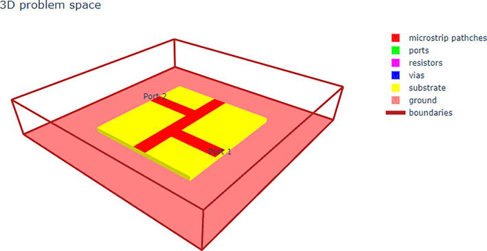
Figure 1.

The geometry of a low-pass filter presented in Sheen et al. [12].

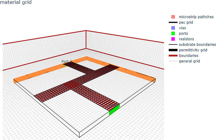
Figure 2.

Material mesh display of the circuit in Figure 1.

As the next step, “initialize_updating_coefficients_and_fields()” function is called to create three-dimensional coefficient and field arrays. For instance, Listing 2 shows the section of the code that is used to create the general coefficient arrays based on (13). In addition to the general updating coefficients, ports and absorbing boundaries as well are set up at this stage.

Listing 2. Section of the code that creates the general coefficient arrays.

Cexe = (2 .* eps_r_x .* eps_0 .- dt .* sigma_e_x)

    ./(2 .* eps_r_x .* eps_0 .+ dt .* sigma_e_x);

Cexh = (2*dt*dx/(dy*dz))

    ./ (2 .* eps_r_x .* eps_0 .+ dt .* sigma_e_x);

Ceye = (2 .* eps_r_y .* eps_0 .- dt .* sigma_e_y)

    ./(2 .* eps_r_y .* eps_0 .+ dt .* sigma_e_y);

Ceyh = (2*dt*dy/(dx*dz))

    ./(2 .* eps_r_y .* eps_0 + dt .* sigma_e_y);

Ceze = (2 .* eps_r_z .* eps_0 .- dt .* sigma_e_z)

    ./ (2 .* eps_r_z .* eps_0 + dt .* sigma_e_z);

Cezh = (2*dt*dz/(dx*dy))

    ./ (2 .* eps_r_z .* eps_0 + dt .* sigma_e_z);

Chxe = dt*dx/(dy*dz*mu_0)

Chye = dt*dy/(dz*dx*mu_0)

Chze = dt*dz/(dx*dy*mu_0)

It should be noted that all three-dimensional arrays that represent fields as well as coefficients are of data type Float32 in the presented Julia code, which is the single-precision floating-point format that occupies 32 bits in computer memory. Generally double-precision floating-point numbers are used in scientific computation due to the higher accuracy it can provide. However, our experience shows that single-precision numbers are sufficient for the most time to achieve sufficiently accurate results in FDTD simulations. In general single-precision arithmetic is faster-than double-precision arithmetic and single-precision can safely be preferred to achieve faster execution of the program in the case of FDTD.

When initializing the ports, data structures for a voltage source, a captured voltage and a captured current at the port location are created for each port. In this code the waveform to excite a voltage source is created as the derivative of Gaussian waveform by default. This waveform is a wideband waveform in its frequency spectrum while excluding very low frequencies and it can lead to faster simulation in which the transients can vanish quickly. The code can be easily modified to accommodate Gaussian, cosine modulated Gaussian, or any other custom waveform that can be used to excite a voltage source.

The next step is to run the time marching loop in “run_time_marching_loop()”, part of which is shown in Listing 3. Notice that since the main goal of the FDTD analysis of a microstrip circuit is to obtain its scattering parameters, the time marching loop needs to be repeated for each port. Each time one port needs to be active as the source port while other sources are inactive. The voltage source of the active port is excited during the time marching loop, and voltages and currents are captured at all ports and stored in their respective arrays to be used during a post-processing step later. Each time the time marching iterates until transient fields are sufficiently vanished or the maximum number of time steps indicated in the project file is reached. In the given code, transient voltage that is captured at the source port is evaluated to determine if the transients vanished sufficiently; if the sum of the absolute values of voltages in the last 200 time steps is less than a value chosen as the stopping criterion then the time marching loop is ended.

Listing 3. Code showing the time marching loop executed for each active port.

for active_port in 1:number_of_ports

  if (!ports[active_port].is_active)

   continue

  end

  println("<Running port $active_port of $number_of_ports ports>")

  clear_fields(Ex, Ey, Ez, Hx, Hy, Hz, pml_boundary)

  vs = ports[active_port].voltage_source

  vf = v_fields[active_port]

  for time_step = 1:number_of_time_steps

    if (check_convergence(ports, active_port, time_step))

     break

    end

  update_Hx(Hx, Chxe, Ey, Ez, nx, ny, nz, nxp1, nyp1, nzp1)

  update_Hy(Hy, Chye, Ez, Ex, nx, ny, nz, nxp1, nyp1, nzp1)

  update_Hz(Hz, Chze, Ex, Ey ,nx, ny, nz, nxp1, nyp1, nzp1)

  update_Hx_PML(Hx, Chxe, Ey, Ez, nx, ny, nz,

           nxp1, nyp1, nzp1, pml_boundary)

  update_Hy_PML(Hy, Chye, Ez, Ex, nx, ny, nz,

           nxp1, nyp1, nzp1, pml_boundary)

  update_Hz_PML(Hz, Chze, Ex, Ey, nx, ny, nz,

           nxp1, nyp1, nzp1, pml_boundary)

  capture_sampled_currents(ports, Hx, Hy,

           active_port, time_step)

  update_Ex(Ex, Cexe, Cexh, Hz, Hy, nx, ny, nz,

           nxp1, nyp1, nzp1)

  update_Ey(Ey, Ceye, Ceyh, Hx, Hz, nx, ny, nz,

           nxp1, nyp1, nzp1)

  update_Ez(Ez, Ceze, Cezh, Hy, Hx, nx, ny, nz,

           nxp1, nyp1, nzp1)

  update_Ex_PML(Ex, Cexe, Cexh, Hz, Hy, nx, ny, nz,

           nxp1, nyp1, nzp1, pml_boundary)

  update_Ey_PML(Ey, Ceye, Ceyh, Hx, Hz, nx, ny, nz,

           nxp1, nyp1, nzp1, pml_boundary)

  update_Ez_PML(Ez, Ceze, Cezh, Hy, Hx, nx, ny, nz,

           nxp1, nyp1, nzp1, pml_boundary)

  update_voltage_sources(vs, vf, time_step)

  capture_sampled_voltages(ports, v_fields,

           active_port, time_step)

  end

end

During each iteration of the time marching loop, first, magnetic fields $H_x$, $H_y$, and $H_z$ are updated each by calling a respective function. For instance, Listing 4 shows the function “update_Hx()” to update $H_x$ based on the Eq. (14). Notice that the coefficient “Chxe” is a scalar here.

After magnetic fields are updated in the entire three-dimensional space, magnetic fields are updated on the boundaries based on the ADE-PML boundary conditions equations. Next, values of currents are captured at all ports using the newly updated magnetic fields.

Listing 4. The function that updates $H_x$.

function update_Hx(Hx, Chxe, Ey, Ez,nx, ny, nz, nxp1, nyp1, nzp1)

  Hx[1:nxp1,1:ny,1:nz] .= (Hx[1:nxp1,1:ny,1:nz]

    .+ Chxe .* (Ey[1:nxp1,1:ny,2:nzp1] .- Ey[1:nxp1,1:ny,1:nz]

    .- Ez[1:nxp1,2:nyp1,1:nz] .+ Ez[1:nxp1,1:ny,1:nz]));

end

Then the iteration proceeds to compute electric fields $E_x$, $E_y$, and $E_z$ by calling a respective function for each. For instance, Listing 5 shows the function “update_Ex()” to update $E_x$ based on the Eq. (13). Notice that the coefficients “Cexe” and “Cexh” both are three-dimensional arrays here.

Listing 5. The function that updates $E_x$.

function update_Ex(Ex, Cexe, Cexh, Hz, Hy,nx, ny, nz, nxp1, nyp1, nzp1)

  Ex[1:nx,2:ny,2:nz] .= (Cexe[1:nx,2:ny,2:nz] .* Ex[1:nx,2:ny,2:nz]

         .+ Cexh[1:nx,2:ny,2:nz] .* (Hz[1:nx,2:ny,2:nz]

         .- Hz[1:nx,1:ny-1,2:nz] .- Hy[1:nx,2:ny,2:nz]

         .+ Hy[1:nx,2:ny,1:nz-1]));

End

After electric fields are updated in the entire three-dimensional space, electric fields are updated on the boundaries based on the ADE-PML boundary conditions equations. Next, electric fields are updated due to voltage source excitation at the location of the active port. Then the values of voltages are captured at all ports using the newly updated electric fields.

Once the time marching loops are completed, all transient voltages and currents that are captured at all ports for all port excitations are available to perform post processing. The “calculate_scattering_parameters()” function is called to compute the scattering parameters.

As the last step of the FDTD simulation, the “display_simulation_results()” function is called to display all transient voltages and currents captured during the FDTD simulation as well as the scattering parameters computed in the post processing step. We will show such results in the next section.

4. Example circuits simulated in Julia FDTD

In this section we will present simulations of two example microstrip circuits. The first circuit is a low pass microstrip circuit that is illustrated in Figure 2. Listing 6 shows the XML file that is used to set up the analysis for this circuit. In this file the cell size is set as $\mathit{\Delta x}=0.4064\mathit{mm}$, $\mathit{\Delta y}=0.4233\mathit{mm}$, and $\mathit{\Delta z}=0.265\mathit{mm}$. The substrate has a dielectric constant of ${\epsilon }_r=2.2$ and a thickness of $\mathit{\Delta h}=0.795\mathit{mm}.$The maximum number of time steps to run the simulation is 4000. The size and position of the substrate and microstrip patches are listed as coordinates of rectangular shapes. Port 1 is set active while Port 2 is inactive, such as to simulate Port 1 excitation only to obtain the scattering parameters $S_{11}$ and $S_{21}$. The Julia program is executed by calling “run_fdtd(“low_pass_filter.xml”)”.

For this example, the program reached the stopping criterion at about 3700 time steps. Then the simulation results are generated as plots. Figure 3 shows the voltage waveform generated by the Port 1 voltage source as well as the transient voltages captured at Port 1 and Port 2 up to 1 nano seconds. Figure 4 shows the scattering parameters on a frequency range 0.5 GHz to 20 GHz.

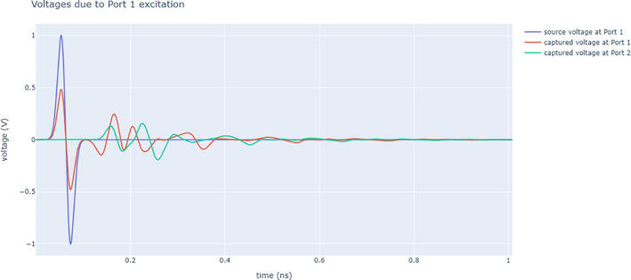
Figure 3.

Transient voltages captured due to port 1 excitation.

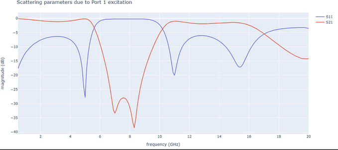
Figure 4.

Scattering parameters of the low pass filter on a range 0.5 GHz to 20 GHz.

The second example, shown in Figure 5, is a bandpass filter presented in Hong [13] (in Figure 5.27). This filter is designed based on a five-pole Chebyshev lowpass prototype with a 0.1-dB passband ripple. For the microstrip filter design, a dielectric substrate with a relative dielectric constant of ${\epsilon }_r=10.2$ and a thickness of $\mathit{\Delta h}=0.635\mathit{mm}$ is used. Listing 7 is a section of the XML file that is used to set up simulation of this band pass filter and it shows how the geometry of the microstrip circuit is created using a polygon and multiple vias. For the FDTD simulation of this circuit a cell size of $\mathit{\Delta x}=0.2\mathit{mm}$, $\mathit{\Delta y}=0.2\mathit{mm}$, and $\mathit{\Delta z}=0.1585\mathit{mm}$ is used. Figure 6 shows the scattering parameters calculated after 40,000 time steps.

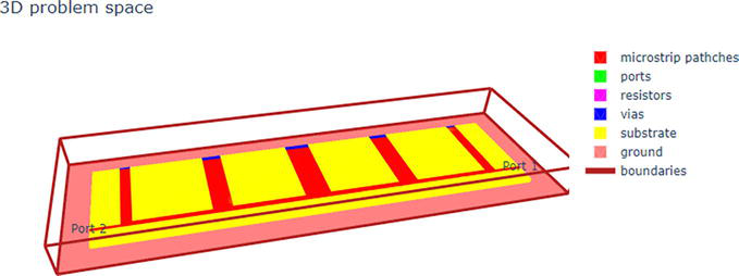
Figure 5.

The geometry of a band pass filter presented in Hong [13].

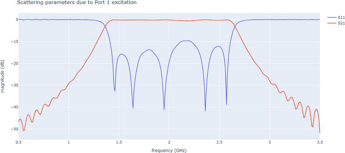
Figure 6.

Scattering parameters of the band pass filter on a range 0.5 GHz to 3.5 GHz.

Listing 6. XML file that is used to set up simulation of a low pass filter.

<?xml version="1.0" encoding="UTF-8"?>

<project>

<analysis_setup>

  <dx>0.4064e-3</dx>

  <dy>0.4233e-3</dy>

  <dz>0.265e-3</dz>

  <maximum_number_of_time_steps>4000</maximum_number_of_time_    steps>

  <courant_factor>0.9</courant_factor>

</analysis_setup>

<geometry>

  <substrate>

    <relative_permittivity>2.2 </relative_permittivity>

    <electric_conductivity>0.0 </electric_conductivity>

    <thickness>0.795e-3 </thickness>

    <min_coordinate> 0 0 </min_coordinate>

    <max_coordinate> 0.0203 0.0195 </max_coordinate>

  </substrate>

  <rectangle>

    <min_coordinate> 0 0.0085 </min_coordinate>

    <max_coordinate> 0.0203 0.011 </max_coordinate>

  </rectangle>

  <rectangle>

    <min_coordinate> 0.0056896 0.0 </min_coordinate>

    <max_coordinate> 0.008128 0.0085 </max_coordinate>

  </rectangle>

  <rectangle>

    <min_coordinate> 0.012192 0.0085 </min_coordinate>

    <max_coordinate> 0.0146304 0.0195 </max_coordinate>

  </rectangle>

</geometry>

<sources>

  <port>

     <min_coordinate> 0.012192 0.0195 </min_coordinate>

     <max_coordinate> 0.0146304 0.0195 </max_coordinate>

     <impedance> 50 </impedance>

     <is_active> 1 </is_active>

  </port>

  <port>

     <min_coordinate> 0.0056896 0.0 </min_coordinate>

     <max_coordinate> 0.008128 0.0 </max_coordinate>

     <impedance> 50 </impedance>

     <is_active> 0 </is_active>

  </port>

</sources>

<outputs>

  <frequencies>

     <start>0.5e9</start>

     <end>20e9</end>

     <step>0.1e9</step>

  </frequencies>

</outputs>

</project>

5. Conclusions

In this chapter we presented an implementation of the FDTD method in Julia customized to simulate microstrip circuits. The code of this implementation is accessible at [11]. The code can be downloaded and used as a base code to experiment with various features of the FDTD method and it can be optimized for more efficient execution following the best practices and performance tips for Julia.

It should be noted that the most effective method to improve the efficiency of a program is to utilize the parallel processing capabilities of the computer system on which the program is running. Julia supports four categories of concurrent and parallel programming, which are asynchronous tasks or coroutines, multi-threading, distributed computing, and GPU computing. It is highly recommended to utilize these parallel processing capabilities supported by Julia based on the available computer architecture.

Listing 7. Part of the XML file that is used to set up simulation of the band pass filter.

<geometry>

  <substrate>

     <relative_permittivity>10.2 </relative_permittivity>

     <electric_conductivity>0.0 </electric_conductivity>

     <thickness > 0.635e-3 </thickness>

     <min_coordinate> −0.03324 0 </min_coordinate>

     <max_coordinate>0.03324 0.018 </max_coordinate>

  </substrate>

  <polygon>

     <vertex> −0.03324 0.01441 </vertex>

     <vertex> −0.02904 0.01441 </vertex>

     <vertex> −0.02904 0 </vertex>

     <vertex> −0.02743 0 </vertex>

     <vertex> −0.02743 0.01403 </vertex>

     <vertex> −0.01594 0.01403 </vertex>

     <vertex> −0.01594 0 </vertex>

     <vertex> −0.01294 0 </vertex>

     <vertex> −0.01294 0.0139 </vertex>

     <vertex> −0.001965 0.0139 </vertex>

     <vertex> −0.001965 0 </vertex>

     <vertex> 0.001965 0 </vertex>

     <vertex> 0.001965 0.0139 </vertex>

     <vertex> 0.01294 0.0139 </vertex>

     <vertex> 0.01294 0 </vertex>

     <vertex> 0.01594 0 </vertex>

     <vertex> 0.01594 0.01403 </vertex>

     <vertex> 0.02743 0.01403 </vertex>

     <vertex> 0.02743 0 </vertex>

     <vertex> 0.02904 0 </vertex>

     <vertex> 0.02904 0.01441 </vertex>

     <vertex> 0.03324 0.01441 </vertex>

     <vertex> 0.03324 0.015 </vertex>

     <vertex> −0.03324 0.015 </vertex>

   </polygon>

<via>

   <min_coordinate> −0.02904 0 </min_coordinate>

   <max_coordinate> −0.02743 0.00036 </max_coordinate>

</via>

<via>

   <min_coordinate> −0.01594 0 </min_coordinate>

   <max_coordinate> −0.01294 0.00083 </max_coordinate>

</via>

<via>

   <min_coordinate> −0.001965 0 </min_coordinate>

   <max_coordinate>0.001965 0.00087 </max_coordinate>

</via>

<via>

   <min_coordinate>0.01294 0 </min_coordinate>

   <max_coordinate>0.01594 0.00083 </max_coordinate>

</via>

<via>

   <min_coordinate>0.02743 0 </min_coordinate>

   <max_coordinate>0.02904 0.00036 </max_coordinate>

</via>

</geometry>

References

- 1.
Yee K. Numerical solution of initial boundary value problems involving maxwell’s equations in isotropic media. IEEE Transactions on Antennas and Propagation. 1966; 14 (3):302-307 - 2.
Taflove A, Hagness SC. Computational Electrodynamics: The Finite-Difference Time-Domain Method. 3rd ed. Norwood, MA: Artech House; 2005 - 3.
Elsherbeni A, Demir V. The Finite-Difference Time-Domain Method for Electromagnetics with MATLAB® Simulations: ACES Series. 2nd ed. Edison, NJ: Scitech Publishing; 2015 - 4.
Sullivan DM. Electromagnetic Simulation Using the FDTD Method. Piscataway, NJ: John Wiley & Sons; 2013 - 5.
Gedney S. Introduction to the Finite-Difference Time-Domain (FDTD) Method for Electromagnetics. Vol. 6. 2011. pp. 227-230 - 6.
The Julia Programming Language. Available from: https://julialang.org/ - 7.
Bezanson J, Edelman A, Karpinski S, Shah VB. Julia: A fresh approach to numerical computing. SIAM Review. 2017; 59 (1):65-98. DOI: 10.1137/141000671 - 8.
Gedney SD, Zhao B. An auxiliary differential equation formulation for the complex-frequency shifted PML. IEEE Transactions on Antennas and Propagation. 2010; 58 (3):838-847 - 9.
Liao Z, Huang K, Yang BP, Yuan YF. A transmitting boundary for transient wave analyses. Science in China Series A-Mathematics, Physics, Astronomy & Technological Science. 1984; 27 :1063-1076 - 10.
Mur G. Absorbing boundary conditions for the finite-difference approximation of the time-domain electromagnetic-field equations. IEEE Transactions on Electromagnetic Compatibility. 1981; EMC-23 (4):377-378 - 11.
FDTD in Julia. Available from: http://www.sosine.net/ - 12.
Sheen DM, Ali SM, Abouzahra MD, Kong JA. Application of the three-dimensional finite-difference time-domain method to the analysis of planar microstrip circuits. IEEE Transactions on Microwave Theory and Techniques. 1990; 38 (7):849-857 - 13.
Hong JS. Microstrip Filters for RF/Microwave Applications. Wiley Series in Microwave and Optical Engineering. Hoboken, NJ: Wiley; 2010