Novel Approaches for Point Cloud Analysis with Evidential Methods: A Multifaceted Approach to Object Pose Estimation, Point Cloud Odometry, and Sensor Registration

Abstract

Autonomous agents must understand their environment to make decisions. Perception systems often interpret point cloud measurements to extract beliefs about their surroundings. A common strategy is to seek beliefs that are least likely to be false, commonly known as cost-based approaches. These metrics have limitations in practical applications, such as in the presence of noisy measurements, dynamic objects, and debris. Modern solutions integrate additional stages such as segmentation to counteract these limitations, thereby increasing the complexity of the algorithms while being internally flawed. An alternative strategy is to extract beliefs that are best supported by the data. We call these evidence-based methods. This difference allows for robustness to the limitations of using cost-based methods without needing complex additional stages. Essential perception tasks such as object pose estimation, point cloud odometry, and sensor registration are solved using evidence-based methods. The demonstrated approaches are simple, require minimum configuration and tuning, and circumvents the need for additional processing stages.

1. Introduction

A fundamental capability for robotic agents is the capacity to perceive the environment in which they operate. This capability is often achieved via the interpretation of point cloud measurements provided by onboard sensors such as Light Detection And Ranging (LiDAR). The established beliefs must be robust, accurate and time-bounded, as they are used to inform control actions.

A popularized strategy for extracting beliefs from point cloud measurements is to fit data to a hypothesis, that is, accepting the hypothesis that best validates the data. We call these strategies ‘cost-based methods’, e.g. the Iterative Closest Point (ICP) method [1, 2]. A fundamentally different strategy is to fit the hypothesis to the data, that is, accepting the hypothesis that would most likely reproduce the data. We call these strategies ‘evidence-based methods’, e.g. the Normal Distributions Transform (NDT) method [3].

At a surface level, it may seem that these strategies are the same thing worded differently, however, the two approaches yield very different solutions, with the latter being much more robust to challenges arising in real-world applications. In non-segmented data, any hypothesized belief will appear improbable of reproducing the complete measurement set. Our proposed evidence-based strategies accept improbable beliefs so long as they are the most probable. As Sherlock Holmes suggests [4], “… and improbable as it is, all other explanations are more improbable still.”

This chapter demonstrates how Evidence-based methods can be used to address three common perception problems that arise in the interpretation of point cloud measurements. These are:

1. Object pose estimation: Robotic agents often need to find and interact with known geometries in their environment. This problem involves estimating the pose, ${\widehat{\mathbf{T}}}_{\mathcal{S}\to \mathcal{M}}$, of a known geometry model described in a model-fixed frame, $\mathcal{M}$, relative to a sensor (or other) coordinate frame, $\mathcal{S}$ (see Figure 1a).

2. Point cloud odometry: This problem arises whereby a robotic agent needs to know it’s location within an established map. We formulate this as finding the pose, ${\widehat{\mathbf{T}}}_{\mathcal{M}\to \mathcal{S}}$, that best fits a new point cloud, ${\mathbf{Z}}_{\mathcal{S}}$, to an existing point cloud map, ${\mathbf{Z}}_{\mathcal{M}}$ (see Figure 1b).

3. Sensor registration: Extrinsic calibration, or sensor registration, involves estimating a sensor’s pose, ${\widehat{\mathbf{T}}}_{\mathcal{P}\to \mathcal{S}}$, relative to a platform coordinate frame, $\mathcal{P}$. We provide a method that seeks to provide consistency between $m$ scans, ${\mathbf{Z}}_{{\mathcal{S}}_{1:m}}$, taken from $m$ platform poses, ${\mathbf{T}}_{\mathcal{W}\to {\mathcal{P}}_{1:m}}$, that are known within a World coordinate frame, $\mathcal{W}$ (see Figure 1c).

Figure 1.

This chapter demonstrates evidential methods towards three candidate problems that commonly arise in the interpretation of point cloud measurements. Namely, the estimation of: (a) an object’s pose, ${\widehat{\mathit{T}}}_{\mathcal{S}\to \mathcal{M}}$, within a point cloud; (b) a platform or sensor’s location, ${\widehat{\mathit{T}}}_{\mathcal{M}\to \mathcal{S}}$, within a map; and (c) a sensor’s installed pose, ${\widehat{\mathit{T}}}_{\mathcal{P}\to \mathcal{S}}$, aboard a moving platform.

This chapter explores the transformative potential of using evidential methods in point cloud analysis. Section 2 explores the state-of-the art where cost and evidence approaches are employed. Several challenges that occur in extracting beliefs from point cloud data are presented in Section 3. Particular attention is shown as to why these challenges present predictable failure modes to cost-based methods but do not inhibit evidence-based methods. Section 4 demonstrates how evidence is established from point cloud data to support hypotheses about the environment. The use of evidential methods are then demonstrated against the three candidate problems of pose estimation, localization, and sensor registration in Sections 5-7. Concluding remarks are made in Section 8.

2. Background and introduction to relevant literature

This section introduces the idea behind cost and evidence-based metrics, followed by exploring existing approaches to solving the three problems introduced previously, using cost, evidence, and learning-based approaches.

2.1 Commonalities in the three perception problems

The object pose estimation, localization and mapping, and sensor registration problems involve matching or aligning two inputs to estimate a homogeneous transform. We denote the two inputs as a source and reference, as is commonly used in existing literature. For the object pose estimation problem, the source is a point cloud and the reference is a known geometry, with the task of locating the known geometry in the point cloud. The geometry may be represented as a triangulated mesh or a sampled point cloud of the mesh. For the localization problem, both the source and reference are point clouds, used to estimate the transform of the sensor between both point clouds. The sensor registration problem is slightly different in that it aims to find the rigid transform between the sensor and the platform frame. Still, it aims to accurately align a series of point clouds to uncover the unknown transform.

2.2 Cost-based vs. evidence-based metrics

Approaches to solving these problems generally follow a similar structure consisting of two main components – (1) an objective function that provides a quantitative metric to differentiate pose hypotheses, whether this be the pose or configuration of an object in a point cloud, the pose between two point clouds, or the pose from the platform to the sensor used to align scans, and, (2) a search algorithm used to find the hypothesis that provides the best result from the objective function. Here, we focus on the first component, the objective function.

Figure 2 illustrates a simple example of an object pose estimation to introduce and highlight the distinction between cost and evidence-based approaches. Cost-based approaches penalize scan points for being located further away from the source. Figure 2a shows the cost map for a known geometry in a hypothesized pose, ${\widehat{\mathbf{T}}}_{\mathcal{S}\to \mathcal{M}}$. Scan points close to the geometry incur a low cost, whereas points located further away have a higher cost. This is intuitive in that corresponding points in the scan and model will obtain zero error if they are closely aligned and a large error otherwise. This assumption only holds if all points correspond to the model, i.e. the point cloud is segmented. Figure 2c, shows the resulting estimate of a cost-based metric in a non-segmented point cloud. Locating the geometry with the true solution is unfavourable by the cost metric as the non-model points incur a high cost. This problem is overcome by using an evidence-based metric where there is no consequence for having non-model points in the scene. Figure 2b displays the evidence map for the same geometry located via the same estimate. Scan points located close to the geometry provide high evidence, whereas points located further from the geometry provide no evidence. This allows for accurate alignment as shown in Figure 2d. The difference allows for a robust foundation for solving the three problems explored in this chapter.

Figure 2.

An object pose estimation problem used to illustrate the distinction between cost and evidence-based metrics. A cost map of a known geometry, $\mathcal{M}$, is shown in (a), where points located near the surface incur zero error, with the cost increasing away from the surface. Non-model points detract from the true pose leading to misalignment. The minimum cost solution, ${{\mathit{T}}^{\star }}_{\mathcal{S}\to \mathcal{M}}$, is shown in (c). The evidence-based metric, shown in (b), overcomes this limitation as points located near the surface contribute high evidence whereas points located further from the surface do not contribute any evidence. The maximum evidence solution, ${{\mathit{T}}^{\star }}_{\mathcal{S}\to \mathcal{M}}$, is shown is shown in (d).

2.3 Cost-based approaches

The most common and prominent example of a cost-based approach is the Iterative Closest Point (ICP) algorithm proposed by Chen and Medioni [2] and Besl and McKay [1]. ICP introduced a simple and efficient method for solving object pose estimation and scan alignment problems, predicated on the belief that the best alignment between two scans or a scan and a geometry is given when the point-to-point distance between the reference and source is minimized. Mathematically, ICP aims to find the homogeneous transform, ${\widehat{\mathbf{T}}}_{\mathcal{S}\to \mathcal{M}}^{\star }$, that minimizes point-to-point/point-to-model distances when applied to the scan, ${\mathbf{Z}}_{\mathcal{S}}$,

$${\mathbf{T}}_{\mathcal{S}\to \mathcal{M}}^{\star }=\underset{j}{argmin}\left\{\sum _{i=1}^n\Vert z_{i\mid j}-r_k\Vert \right\},$$E1

where $z_{i\mid j}$ is the $i$-th point of the scan located by the $j$-th hypothesis, ${\widehat{\mathbf{T}}}_{\mathcal{S}\to \mathcal{M},j}$, and where $r_k$ is the closest reference point to $z_{i\mid j}$. ICP is independent of shape representation and normally distributed noise, however, the application finds significant limitations when used with real-world data. Nevertheless, the past 30 years have seen the rising application of ICP as the foundation for many algorithms with an increasing number of additional stages to overcome its limitations. For example, Sun et al. [5] use fast point feature histograms to decrease ICP’s sensitivity to the initial guess, Yu et al. [6] introduce pre-processing filters to denoise the scans to achieve a more accurate alignment, and Zhang et al. [7] propose pose search efficiencies to achieve real-time performance. Donoso et al. [8] explore the performance of 20,637 variants of ICP for scan matching terrain point clouds and find that no single variant satisfies all criteria. They proceed to propose three new variants to meet the required performance [9]. Pomerleau et al. [10] and Rusinkiewicz and Levoy [11] illustrate the recursive spawning of variants to tailor the ICP implementation to the application, increasing the complexity and failure mechanisms of the algorithm.

2.4 Evidence-based approaches

Evidence-based approaches model the problem as a maximum likelihood estimation problem. These methods claim to overcome many of the core limitations of ICP while improving the accuracy and timeliness of solutions. Two prominent approaches include the Coherent Point Drift (CPD) method by Myronenko and Song [12] and the Normal Distributions Transform (NDT) by Biber and Strasser [3]. CPD handles both rigid and non-rigid point cloud-to-point cloud matching by representing each set of points as a Gaussian Mixture Model and searching for the transform that maximizes the likelihood when the two sets are aligned. The approach demonstrates state-of-the-art performance in noisy and cluttered environments, however, it is computationally expensive. NDT aims to find the homogeneous transform, ${\mathbf{T}}_{\mathcal{S}\to \mathcal{M}}^{\star }$, that maximizes per point likelihood,

$${\mathbf{T}}_{\mathcal{S}\to \mathcal{M}}^{\star }=\underset{j}{argmax}\left\{\sum _{i=1}^{n}exp\left(\frac{-{\left(z_{i\mid j}-q_i\right)}^{\mathrm{t}}{\mathrm{\Sigma }}_i^{-1}\left(z_{i\mid j}-q_i\right)}{2}\right)\right\}.$$E2

where, $q_i$ and ${\mathrm{\Sigma }}_i$ correspond to the local mean and covariance for $z_{i\mid j}$ respectively. The distinction between cost and evidence-based metrics is evident by comparing Eqs. (1) and (2). NDT provides robustness to noise and clutter, however, it is sensitive to a grid size parameter used to establish local distributions [13]. The authors note that the selection of the grid size parameter depends on the shape of the input data and its application [14].

2.5 Learning-based approaches

Recently, deep learning frameworks have been integrated with fine registration methods such as ICP and NDT to provide faster convergence without the requirement of a good initial pose. Ahmdali et al. [15] use deep learning to match features in the source and reference to decrease computation time and provide a coarse guess for the finer registration process using ICP. The solution provides improved performance with significant occlusions and minimal overlap. Wang and Solomon [16] demonstrate state-of-the-art performance with Deep Closest Point. Their proposed pipeline uses a Dynamic Graph CNN and an attention module to extract correspondences required to estimate the rigid transform between the source and reference. However, there are two main disadvantages of learning-based approaches that limit their usability in applications requiring functionally safe performance. Firstly, the performance relies on having sufficient training data for accurate performance, and secondly, understanding failure mechanisms is difficult with errors not always being traceable through the many layers in a deep-learning network. Ideally, a deterministic and traceable algorithm is required to allow failure modes to be understood and accounted for.

3. Challenges in extracting beliefs from point clouds

Point clouds provide no semantic information about the environment they represent. Extracting beliefs from point cloud data requires interpretation, a process that is challenged by numerous mechanisms, some of which are explored in this section.

3.1 Point clouds contain measurement uncertainty

Several sources of uncertainty are inherent to the measurement process of point cloud sensors. Perception sensors such as LiDAR have documented range measurement uncertainty. There is also uncertainty in the per-beam intrinsic calibration used to describe the elevation and heading of the range measurement [17, 18]. Point cloud measurements are often interpreted in a different coordinate system to the sensor frame. This requires accurate extrinsic calibration (sensor registration) to determine the relative pose between the platform and sensor [19, 20]. It is not reasonable to expect a zero-cost pose solution in light of these sources of measurement uncertainty.

3.2 Point clouds do not arrive with perfect correspondence

Cost-based methods assume correspondence, that is, they assume all source measurements belong to the reference model. This assumption is rarely valid. Figure 3a displays two successive scans captured by a vehicle travelling on a highway. Attempting to match these scans is problematic as not all measurements should appear in both scans. This is because (i) dynamic objects will have moved between scans, and (ii) the new scan will observe a different part of the environment compared to the previous scan. The use of an evidence-based metric alleviates this problem as non-corresponding points do not detract from the true pose being accepted.

Figure 3.

Two key challenges involve extracting beliefs in the presence of dynamic objects and debris. Two successive scans captured onboard a moving vehicle from the KITTI dataset [21] are displayed in (a). Aligning the scans using the relative pose estimate reveals a moving vehicle in the environment. The presence of such dynamic objects corrupts the assumption of static point cloud used for point cloud-to-point cloud matching. A scan captured from a LiDAR mounted to a rope shovel is shown in (b). Dust occludes the view of the shovel’s dipper and the truck.

3.3 Point cloud sensors are susceptible to environmental conditions

Atmospheric obscurants such as dust and fog inhibit the capacity of perception sensors to provide an accurate representation of the environment [22]. Figure 3b shows a scan captured during an excavator’s loading cycle. A large amount of dust is disturbed, presenting as spurious measurements in the point cloud (dark green). Consider the problem of estimating the pose of a haul truck model in the point cloud data. The measurements attributed to dust would inhibit a cost-based metric as they do not correspond to the model and are challenging to automatically segment. An evidence metric would find that these spurious measurements do not support the true pose of the truck, however, they do not detract from the true pose being accepted, hence bypassing the need to segment measurements attributed to atmospheric obscurants.

3.4 Real-time point cloud processing is challenging

It is challenging to extract beliefs in real time from high-density point cloud measurements. Point clouds generated by common sensors such as the Ouster OS1-64 provide up to 2,621,440 points per second [23]. Interpreting point clouds of this size presents a bottleneck for most algorithms. Reducing the number of points by subsampling the data using radial or voxel-based approaches allows for faster processing at the cost of reduced information about the scene. Due to the lack of semantic information, algorithms often require multiple pre-processing filters to clean the scan before use. For example, several algorithms perform ground plane fitting [24] to identify and segment ground points and use the remaining point cloud for interpretation. In the sections that follow, we provide computationally efficient approximations of evidence that enable real-time interpretation.

4. Evidential methods in point cloud analysis

This section introduces the concept of evidential methods in point cloud analysis. It explores the notion of ray-based evidential analysis, including the construction of a per-point “evidential” and the principle of Maximum Sum of Evidentials. These ideas are originally presented in [25].

4.1 How does a point provide evidence towards a hypothesis?

Evidential methods are predicated on the belief that the likelihood of an estimate is correlated with the likelihood of reproducing the observed measurements. The likelihood of reproducing point cloud measurements can be ascertained via a sensor measurement model. Here, we consider the measurement model of a range-scanning LiDAR sensor. A LiDAR sensor produces range measurements over a set of beam heading and elevation angles. The expected range measurements are obtained by raycasting against a hypothesized environment, $\mathbf{H}$. Figure 4a depicts the raycasting operation performed along the $i$-th beam against the $j$-th environment hypothesis, ${\mathbf{H}}_{\mathbf{j}}$. The raycasted range measurement, ${\widehat{z}}_{i\mid j}$, is directly comparable to the observed measurement, $z_i$, along the same beam. In this case, it is shown to be a slightly longer range.

Figure 4.

(a) A geometry model is located with an assumed Hypothesis, ${\mathit{H}}_j$. Under this hypothesis, the measurement ${\widehat{z}}_{i\mid j}$ would be observed along the $i$-th beam. (b) The likelihood of observing $z_i$ conditional to the hypothesis ${\mathit{H}}_j$ is modelled as $f\left(z_i|{\mathit{H}}_j\right)$ using the sensor’s range uncertainty $\sigma$. Figure from Ref. [25].

The observed measurement, $z_i$, provides a measure of evidential support for the hypothesis, ${\mathbf{H}}_j$. This support is quantified via a conditional range likelihood model, $f\left(z_i|{\mathbf{H}}_j\right)$, describing the likelihood of obtaining measurement $z_i$ conditional to the hypothesis ${\mathbf{H}}_j$ being assumed. This probability density function is established by considering sources of uncertainty in the measuring process of the LiDAR. A simple uncertainty model is to consider the range accuracy of the sensor itself. The measurement uncertainty can be modelled as having a standard deviation, $\sigma$, which is typically in the order of several centimetres. Figure 4b depicts the measurement likelihood model overlayed on the $i$-th beam, calculated as,

$$f\left(z_i|{\mathbf{H}}_j\right)=\mathcal{N}\left(z_i|{\widehat{z}}_{i\mid j},{\sigma }^2\right)=\frac{1}{\sqrt{2{\mathit{\pi \sigma }}^2}}exp\left(-\frac{{\left(z_i-{\widehat{z}}_{i\mid j}\right)}^2}{2{\sigma }^2}\right).$$E3

The measurement likelihood model, $f\left(z_i|{\mathbf{H}}_j\right)$, can be extended to include any source of uncertainty in the measuring process (e.g. those sources of measurement uncertainty discussed in Section 3.1). For example, uncertainty in the sensor’s pose could result in a beam intersecting different locations of the hypothesized environment. We explore these ideas further in [25] where uncertainties (such as intrinsic and extrinsic calibration) are mapped to range likelihood via sampling techniques. However, for most of our work, we have found that the simple model of range uncertainty is sufficient.

4.2 How do we find the hypothesis with the most evidence?

Having established how to evaluate per-point evidence towards a hypothesis, we now seek to determine the hypothesis with the most evidence, ${\mathbf{H}}^{\star }$. We illustrate this problem using the point cloud of $N=9$ range measurements shown in Figure 5a. Here, a robot is parameterized by a two-dimensional hypothesis, ${\mathbf{H}}_j={\left[{\theta }_{1,j},{\theta }_{2,j}\right]}^T$.

Figure 5.

(a) A candidate problem whereby we seek to determine the 2-DOF robot configuration from nine range measurements. (b) The sum of evidence is calculated across the robot configuration workspace with the true hypothesis, ${\mathit{H}}^{\star }$, yielding the highest summation of evidence. (c) An alternate hypothesis ${\mathit{H}}_A$ produces a local maximum of evidence as it is capable of reproducing two-thirds of the range measurements. Figure from Ref. [25].

A brute force approach sums the evidence for all measurements at a finely discretized set of robot configurations across the entire workspace. Doing so produces the surface shown in Figure 5b. A global maximum of evidence is indicated at ${\mathbf{H}}^{\star }=\left[{28.6}^{°}{\mathrm{,114.6}}^{°}\right]$, which also corresponds to the true pose depicted in Figure 5a. This is the basis of evidential point cloud analysis, the hypothesis with the most per-point evidence is the most likely to be true. An alternate hypothesis, indicated by ${\mathbf{H}}_A$, is shown to produce a local maximum of evidence. Figure 5c shows the robot articulated with hypothesis ${\mathbf{H}}_A$. It can be seen that this pose is capable of reproducing six of the nine range measurements. Accordingly, this hypothesis garners two-thirds of the evidence produced by the true solution, ${\mathbf{H}}^{\star }$. Increasing the density of measurements further separates the disparity of evidence between ${\mathbf{H}}^{\star }$ and ${\mathbf{H}}_A$.

4.3 What are the limitations of evidential methods?

The brute force approach presented in the previous section is not a viable approach for time-bounded applications. Raycasting against hypothesized environments is a computationally expensive operation. The number of raycasting operations is proportional to both the number of range measurements and the number of hypotheses tested. It is possible to pre-calculate raycast measurements for a discretized set of hypotheses over a bounded hypothesis space. These precalculated tables of raycast values can then be used to evaluate observed range measurements as they arrive. However, the number of precalculated raycasts quickly increases with the dimensionality of the hypothesis space, making this approach impractical for larger hypothesis spaces.

In the candidate applications that follow, we present the concept of Evidential Rapid Approximation (ERA), a method designed to streamline the computation of evidentials, making the process more viable for real-time applications. For pose estimation (Section 5), we approximate the range likelihood by considering the proximity of point cloud measurements to the surface of a known geometry at a hypothesized pose. Similarly, for localization and mapping (Section 6), evidence is determined by the proximity of new point cloud measurements relative to previously mapped points. Both strategies are an approximation of evidence, neither of which requires the computationally expensive raycasting operation.

5. Applications for object pose estimation – PLuM

The Pose Lookup Method (PLuM) is detailed in Ref. [26] and summarized here.

5.1 Problem overview and applications

The object pose estimation task involves estimating the pose, ${\widehat{\mathbf{T}}}_{\mathcal{S}\to \mathcal{M}}$, of a known geometry described in frame, $\mathcal{M}$, within a point cloud, ${\mathbf{Z}}_{\mathcal{S}}$, captured in the sensor (or other) frame, $\mathcal{S}$. This task is encountered in diverse applications. For example, digital quality inspection matches scans of physical components with a ground truth model to highlight manufacturing defects [27], removing the dependence on Coordinate-Measuring Machines. The bioinformatics industry requires similar algorithms for various tasks such as protein surface matching [28] and retinal image registration [29]. A large area of research is dedicated to body pose estimation dealing with both rigid and deformable models of humans [30], with an application in identifying pedestrians from autonomous vehicles for safer navigation. Numerous use-cases also arise in the automation of mining and agricultural equipment, with the use of object pose estimation for end-effector tracking [31], and identifying known geometries in the workspace from haul trucks [32] to peach trees [33].

The Pose Lookup Method [26], or PLuM, is an approximation of the Maximum Sum of Evidence method described in the previous section that is grounded in ERA. PLuM provides a real-time and accurate method for the 6-DOF pose estimation of known geometries in point cloud data, with extensions to kinematic configuration spaces such as estimating the joint angles for an articulated robot similar to the example displayed in Figure 5. For this application, the source is a point cloud and the reference is a model of the geometry as depicted in Figure 1a, with the objective of finding the ideal transform, ${\mathbf{T}}_{\mathcal{S}\to \mathcal{M}}^{\star }$, that best fits the model to the point cloud data.

5.2 PLuM formulation

PLuM evaluates the per-point evidence using an approximation of Eq. (3), where the difference between the measurement and the raycast measurement, $\left(z_i-{\widehat{z}}_{i\mid j}\right)$, is replaced with the closest distance, $d_{i\mid j}$, between the reference point, $p_{\mathcal{S},i}$, and the model as depicted in Figure 6. The evidence, $e_{i\mid j}$, for point, $p_{\mathcal{S},i}$, is given by a zero-mean Gaussian function,

Figure 6.

(a) PLuM computes the evidence, $e_{i\mid j}$, using a zero-mean Gaussian evaluation of the closest distance between the source point, $p_{\mathcal{S},i}$, and the model, $\mathcal{M}$. (b) A lookup frame, $\mathcal{L}\mathcal{U}$, is rigidly fixed to the model, $\mathcal{M}$, and allows for a direct lookup of evidence for point cloud measurements near the model’s surface. Figure from Ref. [26].

$$e_{i\mid j}=\mathcal{N}\left(d_{i\mid j}|0,{\sigma }^2\right)=\frac{1}{\sqrt{2{\mathit{\pi \sigma }}^2}}exp\left(-\frac{d_{i\mid j}^2}{2{\sigma }^2}\right).$$E4

The evidence is calculated with the user-selected configuration parameter, $\sigma$. The evidence value is at a maximum when the point cloud measurement lies on the surface of the model, corresponding to $d_{i\mid j}=0$, and decreases as the distance between the point cloud measurement and the model increases. As the evidence value is used as a comparative measure between pose hypotheses, the normalisation factor, $\frac{1}{\sqrt{2{\mathit{\pi \sigma }}^2}}$, can be discarded,

$$e_{i\mid j}=exp\left(-\frac{d_{i\mid j}^2}{2{\sigma }^2}\right).$$E5

A major factor inhibiting real-time applicability is the expensive calculation of point-to-model distances, $d_{i\mid j}$, used for the evidence calculation in Eq. (5). PLuM overcomes this limitation by using a pre-computed lookup table of point-to-model distances. Figure 6 depicts the problem and the application of a lookup table used for the evidence calculation. A lookup frame, $\mathcal{L}\mathcal{U}$, is rigidly attached to the geometry to capture a bounding region of pixels (or voxels in 3D) around it. The region is discretized at some resolution, $\mathrm{\Delta }$, with each pixel encoding the closest distance to the geometry. The evidence calculation is performed by the following three steps.

1. The frame transform between the lookup and the sensor frame, ${\widehat{\mathbf{T}}}_{\mathcal{L}\mathcal{U}\to \mathcal{S}\mid j}$, is calculated using the $j$-th pose hypothesis, ${\widehat{\mathbf{T}}}_{\mathcal{S}\to \mathcal{M},j}$, and the known rigid transform from the model to the lookup table, ${\mathbf{T}}_{\mathcal{M}\to \mathcal{L}\mathcal{U}}$,

   $${\widehat{\mathbf{T}}}_{\mathcal{L}\mathcal{U}\to \mathcal{S}\mid j}={\left({\widehat{\mathbf{T}}}_{\mathcal{S}\to \mathcal{M},j}{\mathbf{T}}_{\mathcal{M}\to \mathcal{L}\mathcal{U}}\right)}^{-1}.$$E6

2. The $i$-th point in the source point cloud frame, $p_{\mathcal{S},i}$, is calculated in the lookup frame as,

   $$p_{\mathcal{L}\mathcal{U},i}={\widehat{\mathbf{T}}}_{\mathcal{L}\mathcal{U}\to \mathcal{S}\mid j}{p}_{\mathcal{S},i}={\left[\begin{array}{c}{x}_i\\ y_i\\ z_i\\ 1\end{array}\right]}_{\mathcal{L}\mathcal{U}}.$$E7

3. The $x_i$, $y_i$, and $z_i$ values are used to index the pre-calculated distances stored in the lookup table,

$$d_{i\mid j}=\text{lookup}\left(⌊\frac{x_{i,\mathcal{L}\mathcal{U}}}{\mathrm{\Delta }}⌋,⌊\frac{y_{i,\mathcal{L}\mathcal{U}}}{\mathrm{\Delta }}⌋,⌊\frac{z_{i,\mathcal{L}\mathcal{U}}}{\mathrm{\Delta }}⌋\right),$$E8

where $⌊.⌋$ is the floor function and $\mathrm{\Delta }$ is the lookup table resolution.

5.3 Example point cloud-to-model matching

The evidence-based metric offers robustness to clutter, with the use of lookup tables offering a significant increase in speed. A sample result for estimating the 6-DOF pose of a Stanford dragon model to a point cloud with 90% clutter is shown in Figure 7. Similar behaviour to the scenario depicted in Figure 2 is visible, with the ICP solution corrupted due to the presence of clutter, and the evidence-based approach only rewarding points that best support the hypothesis. The 6-DOF pose hypotheses are listed in Table 1.

Figure 7.

A demonstration of using cost-based vs. evidence-based metrics for object pose estimation. The problem is depicted in (a), with a point cloud consisting of 90% clutter and a dragon model located in its true pose (light green model). Vanilla ICP fails to align the dragon’s pose (dark green model in (b)), whereas PLuM accurately aligns the model with the point cloud (dark green model in (c)).

Source	roll [deg]	pitch [deg]	yaw [deg]	x [mm]	y [mm]	z [mm]
True pose	90.000	0.000	0.000	0.180	0.160	0.000
Vanilla ICP	93.011	−2.123	−6.075	0.192	0.155	−0.007
PLuM	89.487	0.785	0.317	0.178	0.157	0.002

Table 1.

The object pose estimation results using Vanilla ICP and PLuM. PLuM provides a significantly better fit compared to ICP.

PLuM provides an accurate and timely approach to answering the ‘where is it?’ question. Open problems remain about identifying the presence of multiple models or the absence of the model from the scene, as the approach described above will always provide an estimate of the model in the scene.

6. Applications for point cloud odometry – SiMpLE

The Simple Mapping and Localisation Estimation (SiMpLE) algorithm is detailed in [34] and summarized here.

6.1 Problem overview

Point cloud odometry is an approach used to localize an autonomous agent within an environment. Successive scans are matched to recover the change in the sensor’s pose as depicted in Figure 1b. Sequential computation of relative poses allows for recursive pose estimation, whereby the pose at time $t_k$ is based on the point cloud at time $t_k$, the previous pose estimate at time $t_{k-1}$, and some history of the previous scans. This is commonly known as the front-end for Simultaneous Localization and Mapping (SLAM) algorithms. Due to the dead-reckoning behaviour, the approach is prone to drift over long sequences with the accumulation of errors. A back-end is typically employed to optimize pose estimates using loop closure constraints. A low-drift front-end is desired for accurate pose estimation and to aid the back-end computation.

Point cloud-to-point cloud matching is based on the assumption of observing similar features in both scans that can be matched to recover the change in the sensor’s pose. This assumes a static environment as features must be consistent to allow for correct matching. However, agents such as autonomous vehicles operate in highly dynamic environments with the presence of pedestrians and other vehicles. The challenges associated with using cost-based metrics discussed in Section 3 arise. Dynamic points corrupting the scan matching process and partial overlap in scans from a moving platform invalidate the assumption of direct correspondence.

6.2 Existing approaches

Existing scan-matching approaches are often augmented with additional stages to overcome these challenges. For example, many approaches such as LOAM [35] and F-LOAM [16] extract geometric features such as lines and planes between scans to aid the scan matching process. MULLS [24] extend this to identifying environment-specific features such as pillars and beams while continuing to utilize ICP at their core for fine registration. Alternative methods augment deep-learning networks to help with feature extraction and dynamic object detection [36, 37, 38]. While these additional stages improve performance, they also increase complexity and the associated burden of configuration. Ideally, a low configuration and accurate odometry solution is required for use-case agnostic applications among various types of sensors and environments.

SiMpLE has the advantage of providing accurate localization in various applications while having a minimum configuration set consisting of only five parameters. In comparison, most existing approaches have a significant configuration burden. For example, CT-ICP [39] has 30 parameters, SuMa [40] has 49 parameters, and MULLS has 107 parameters. Methods such as LOAM and MULLS rely heavily on feature extraction to aid the registration process. This requires significantly more tuning, and the results are sensitive to the application environment. A practical disadvantage of using SiMpLE and similar methods is the requirement of multithreading to achieve real-time performance, as discussed in Section 3.4.

6.3 SiMpLE formulation

Here, we introduce Simple Mapping and Localization Estimation, or SiMpLE [34]. This scan-to-map registration algorithm seeks to maximize per-point evidence, overcoming many limitations associated with classical scan matching algorithms. The algorithm requires a small configuration set. SiMpLE performs three steps to achieve accurate and timely odometry.

1. Input Scan Subsampling: The first step is to subsample the new scan at time $k$ with a user-defined radius, $r_{\mathit{new}}$, to reduce the size of the input point cloud and allow for real-time computation (Figure 8).

2. Point cloud-to-map matching: A pose hypothesis, ${\widehat{\mathbf{T}}}_{1\to k,j}$, is applied to the subsampled point cloud, $P_k^{\prime }$, to locate it within the existing map, $M_{k-1}^{\prime }$. Under this hypothesis, the approximate per-point evidence, $e_{i\mid j}$, for the $i$-th point, $p_{k,i\mid j}^{\prime }$, is calculated by,

   $$e_{i\mid j}=exp\left(-\frac{d_{i\mid j}^2}{2{\sigma }^2}\right),$$E9

   where $d_{i\mid j}$ is the distance to the closest map point, $m_{k,i\mid j}^{\prime }$. The evidence function has a user-selected standard deviation of $\sigma$. A search algorithm is used to find the hypothesis that maximizes the summated of these evidentials.

3. Local map update: The local map is updated with the current point cloud and the registration result from the previous step. The map is again subsampled at a user-defined radius of $r_{\mathit{map}}$ to allow for fast matching in the next step and points outside the sensor’s maximum range at the current pose are truncated to manage the map size.

Figure 8.

(a) The $k$-th subsampled scan, ${\mathit{P}}_{k^{\prime }}$, is located by the $j$-th pose hypothesis, ${\widehat{\mathit{T}}}_{1\to k,j}$. The $i$-th point is depicted as $p_{k,i\mid j}^{\prime }$ and the per-point evidence is calculated using its proximity, $d_{i\mid j}$, to the closest point, $m_{k-1,i\mid j}^{\prime }$, in the existing map, ${\mathit{M}}_{k-1}^{\prime }$. Per-point evidence, $e_{i\mid j}$, is evaluated as a zero-mean Gaussian function of the distance between these points with a user-selected standard deviation, $\sigma$. (b) The selection of $\sigma$ dictates the magnitude of evidence given the distance, $d_{i\mid j}$, between the scan and map points. Figure from Ref. [34].

6.4 Example odometry and mapping result

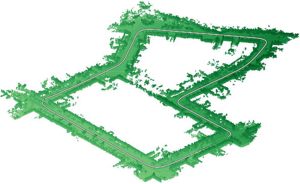
SiMpLE has been extensively tested on public benchmark datasets and performs among state-of-the-art algorithms with with least complex approach and smallest configuration set. An example result of real-time point cloud odometry is shown in Figure 9, using sequence 07 from the KITTI dataset [21]. The trajectory has 0.47% translation error, calculated using the method described in [21]. The vehicle’s trajectory is displayed in white, and the corresponding stitched point cloud map is coloured by the point elevation.

Figure 9.

An example trajectory displayed in white and corresponding point cloud map from the KITTI dataset generated using SiMpLE. The trajectory exhibits low drift over a sequence of 1101 scans. The point cloud map is coloured by elevation.

SiMpLE’s performance can be increased by fusing information from other sensing modalities (e.g. IMU) for providing information in between successive scans. The map currently generated simply stitches successive scans using the pose estimates, disregarding the presence of dynamic elements. SiMpLE can be augmented with dynamic object detection approaches to construct maps of the static environment, as demonstrated in [41]. The open-source approach is available from github.com/vb44/SiMpLE.

7. Application for sensor registration – SeREA

7.1 Problem relevance and description

A frequently occurring requirement for perception is the capacity to represent point cloud measurements in a different coordinate system. This requires accurate knowledge of the frame transform, ${\widehat{\mathbf{T}}}_{\mathcal{P}\to \mathcal{S},j}$, between the desired coordinate system, $\mathcal{P}$, and the sensor coordinate system, $\mathcal{S}$, where the point cloud measurements, ${\mathbf{P}}_{\mathcal{S}}$, are directly provided (Figure 1c). For example, a mobile platform may need to interpret a point cloud to extract obstacles in a platform-fixed coordinate system where the geometry of the platform is described. Alternatively, point cloud measurements can be mapped to a navigation solution (e.g. RTK-GNSS) of the platform frame if the transform between platform and sensor, ${\mathbf{T}}_{\mathcal{P}\to \mathcal{S}}$, is known. The recovery of this transform is often called extrinsic calibration or sensor registration.

The sensor registration problem is commonly addressed using two strategies: (1) methods using a model of the environment and finding the sensor pose that best matches the sensor measurements captured at different positions to the model [20, 42], and (2) model-free approaches that aim to find the sensor pose that best aligns point clouds captured at different sensor poses [19, 43]. D’Adamo et al. [20] evaluate these approaches and find that model-based approaches provide greater accuracy but model-free approaches provide greater convenience by not requiring a model of the environment.

7.2 SeREA formulation

The previous section demonstrated that point clouds could be incrementally added to an existing map using an evidential approach. Hypothesized transforms between the map and scan, ${\mathbf{T}}_{\mathcal{P}\to \mathcal{S}}$, were evidenced if they located new points within proximity to existing map points. The Sensor Registration via Evidential Approximation (SeREA) approach, described here, is established on the same basis. The evidential registration problem is predicated on the belief that the most likely sensor registration, ${\mathbf{T}}_{\mathcal{M}\to \mathcal{S}}^{\star }$, is that which locates points from all scans within proximity to points of all other scans.

The algorithm does not require a survey or model of the environment. It seeks only to provide consistency between successive scans taken at $m$ known platform locations, ${\mathbf{T}}_{\mathcal{W}\to {\mathcal{P}}_1:m}$, within a World coordinate system, $\mathcal{W}$.

The process is as follows:

1. Assuming the $j$-th registration hypothesis, ${\widehat{\mathbf{T}}}_{\mathcal{P}\to \mathcal{S},j}$, locate all scans, ${\mathbf{P}}_{\mathcal{S},1:m}$, within the World coordinate frame, $\mathcal{W}$, using the known platform locations at each scan, ${\mathbf{T}}_{\mathcal{W}\to {\mathcal{P}}_{1:m}}$,

   $${\mathbf{P}}_{\mathcal{W},1:m}={\mathbf{T}}_{\mathcal{W}\to {\mathcal{P}}_{1:m}}{\widehat{\mathbf{T}}}_{\mathcal{P}\to \mathcal{S},j}{\mathbf{P}}_{\mathcal{S},1:m}.$$E10

2. Compute the evidence for each point in ${\mathbf{P}}_{\mathcal{W},1:m}$. The per-point evidence, $p_{\mathcal{W},i}$, under hypothesis, ${\widehat{\mathbf{T}}}_{\mathcal{P}\to \mathcal{S},j}$, is given by,

   $$e_{i\mid j}=exp\left(-\frac{d_{i\mid j}^2}{2{\sigma }^2}\right),$$E11

   where $d_{i\mid j}$ is the distance between point $p_{\mathcal{W},i}$ and its nearest neighbour in ${\mathbf{P}}_{\mathcal{W},1:m}$.

3. The total evidence for the $j$-th hypothesis is given by summating the evidence for each point.

4. The hypothesis space is searched for the pose corresponding to the maximum total evidence.

A pose search algorithm such as a particle filter or gradient-based solver is typically used in the final step when searching for the highest-scoring hypothesis. It is important to note that extracting the 6-DOF extrinsic parameters requires excitation of all degrees of freedom.

7.3 Example extrinsic calibration of a LiDAR mounted to a 6-DOF robot arm

An example is demonstrated below for registering a Velodyne VLP-16 LiDAR to a KUKA KR1000 Titan robotic manipulator. It is critical to accurately register the sensor as beliefs generated using the point cloud need to be transformed into the robot’s frame to allow for interaction with the environment. For example, the robot may be required to identify a known geometry in the environment and then transport it between two locations. If the sensor’s location relative to the robot is incorrect, the estimated object pose will also be incorrectly transformed from the sensor’s frame to the robot’s frame, resulting in failure.

Figure 10a illustrates the problem. The goal is to use a sequence of scans, ${\mathbf{P}}_{{\mathcal{S}}_{1:m}}$, captured in the Sensor frame, $\mathcal{S}$, along with the corresponding pose of the end-effector, ${\mathbf{T}}_{\mathcal{W}\to {\mathcal{P}}_{1:m}}$, in the World frame, $\mathcal{W}$, to estimate the sensor registration, ${\widehat{\mathbf{T}}}_{\mathcal{P}\to \mathcal{S}}$. Figure 9b displays the end-effector’s path over a sequence designed to excite all six degrees of freedom. The platform to sensor 6-DOF registration estimated using SeREA, and the comparison to machine drawings is listed in Table 2.

Figure 10.

A candidate sensor registration problem. (a) We seek to determine the frame transform, ${\widehat{\mathit{T}}}_{\mathcal{P}\to \mathcal{S}}$, that locates the installation of a LiDAR scanner (Sensor frame, $\mathcal{S}$) relative to an end-effector (Platform frame, $\mathcal{P}$). (b) The trajectory of the platform frame is excited in all 6-DOF. A kinematic solution is used to locate it relative to the World frame, $\mathcal{W}$.

Source	roll [deg]	pitch [deg]	yaw [deg]	x [mm]	y [mm]	z [mm]
Machine drawings	0.000	0.000	0.000	−40.000	0.000	250.000
SeREA estimate	0.000	0.082	0.049	−49.815	−4.672	258.851

Table 2.

A comparison of the sensor registration estimate and the machine drawings from which the LiDAR bracket was manufactured.

The machine drawings provide a reference to verify the accuracy of the registration result. In many typical applications, accurate drawings may not be available for comparison. In these circumstances, sensor registration estimation methods such as SeREA are required. Figure 11 shows the resulting map produced with the sensor registration solution applied.

Figure 11.

The registration solution is applied, producing the point cloud shown. The SeREA approach seeks to provide consistency between successive scans.

8. Conclusions

A longstanding approach to interpreting point clouds is to use cost-based solutions. This chapter exposes the limitations of employing cost-based strategies, and promotes an alternative mode of extracting beliefs based in maximizing evidence. This leads to beliefs that are most likely to provide observed point cloud measurements. The change circumvents the need to perform additional processing (e.g. point cloud segmentation), and consequently reduces the complexity of the algorithm.

We formally define evidence as the likelihood of obtaining the observed point cloud measurements. However, this is challenging to use in real-time applications due to the computationally expensive raycasting operation. We demonstrate ways to rapidly approximate evidence and utilize this to provide real-time solutions to three commonly encountered perception problems: (i) PLuM for Pose estimation; (ii) SiMpLE for Scan matching; and (iii) SeREA for Sensor registration. All of which are based in a similar ideology.

The PLuM approach is demonstrated to locate known geometries in unsegmented data. A computational benefit is obtained by shifting from ray-based evidence to Cartesian-based evidence which can be readily looked up in pre-calculated tables. A limitation of this approximation is that it rewards points that are not feasibly obtained along the sensor’s rays, e.g. a point on the opposite side of a model relative to the sensor is not feasible even though it is close to the model. Furthermore, PLuM does not provide diagnostics such as verifying the presence of the model and identifying if the model is different to what is expected.

The SiMpLE approach is shown to accurately map scans together with very low drift. However, the algorithm is unable to identify scenarios when the pose is degraded and due to the recursive nature, a single pose error is sufficient to offset the entire pose trajectory. Back-end methods can be used to correct the trajectory via loop closure.

The SeREA algorithm estimates extrinsic calibration parameters by maximizing the coherence between successive scans. A limitation of this approach is that the sensor needs to be excited in all six degrees of freedom.

The evidential approaches explored in this chapter present a pivotal change in the way beliefs are extracted from point cloud data. The solutions are found to be more robust to existing challenges and require much less configuration than cost-based approaches.

References

1.Besl P, McKay ND. A method for registration of 3-d shapes. IEEE Transactions on Pattern Analysis and Machine Intelligence. 1992;14(2):239-256
2.Chen Y, Medioni G. Object modelling by registration of multiple range images. Image and Vision Computing. 1992;10(3):145-155. Range Image Understanding
3.Biber P, Strasser W. The normal distributions transform: A new approach to laser scan matching. In: Proceedings 2003 IEEE/RSJ International Conference on Intelligent Robots and Systems (IROS 2003) (Cat. No.03CH37453). Vol. 3. New York City, United States: IEEE; 2003. pp. 2743–2748. DOI: 10.1109/IROS.2003.1249285
4.Doyle AC, Paget S. The Adventure of Silver Blaze. UK: Mary McLaughlin and M. Einisman for the Scotland Yard Bookstore; 1979
5.Sun R, Zhang E, Mu D, Ji S, Zhang Z, Liu H, et al. Optimization of the 3d point cloud registration algorithm based on fpfh features. Applied Sciences. 2023;13(5). Available from: https://www.mdpi.com/about/announcements/784
6.Yu Y, Da F, Guo Y. Sparse icp with resampling and denoising for 3d face verification. IEEE Transactions on Information Forensics and Security. 2019;14(7):1917-1927
7.Zhang J, Yao Y, Deng B. Fast and robust iterative closest point. IEEE Transactions on Pattern Analysis and Machine Intelligence. 2022;44(7):3450-3466
8.Donoso F, Austin K, McAree P. How do icp variants perform when used for scan matching terrain point clouds? Robotics and Autonomous Systems. 2017;87:147-161
9.Donoso F, Austin K, McAree P. Three new iterative closest point variant-methods that improve scan matching for surface mining terrain. Robotics and Autonomous Systems. 2017;95:117-128
10.Pomerleau F, Colas F, Siegwart R. A review of point cloud registration algorithms for mobile robotics. Foundations and Trends in Robotics. 2015;4(1):1-104
11.Rusinkiewicz S, Levoy M. Efficient variants of the icp algorithm. In: Proceedings of the 3rd International Conference on 3-D Digital Imaging and Modeling. New York City, United States: IEEE; 2001. pp. 145-152. DOI: 10.1109/IM.2001.924423
12.Myronenko A, Song X. Point set registration: Coherent point drift. IEEE Transactions on Pattern Analysis and Machine Intelligence. 2010;32(12):2262-2275
13.Kaminade T, Takubo T, Mae Y, Arai T. The generation of environmental map based on a ndt grid mapping -proposal of convergence calculation corresponding to high resolution grid. In: 2008 IEEE International Conference on Robotics and Automation. New York City, United States; 2008. pp. 1874-1879. DOI: 10.1109/ROBOT.2008.4543480
14.Magnusson M, Lilienthal A, Duckett T. Scan registration for autonomous mining vehicles using 3d-ndt. Journal of Field Robotics. 2007;24(10):803-827
15.Ahmadli I, Bedada WB, Palli G. Deep learning and octree-gpu-based icp for efficient 6d model registration of large objects. In: Palli G, Melchiorri C, Meattini R, editors. Human-Friendly Robotics 2021. New York City, United States: Springer International Publishing; 2022. pp. 29-43. DOI: 10.1007/978-3-030-96359-0_3. ISBN: 978-3-030-96359-0
16.Wang Y, Solomon JM. Deep closest point: Learning representations for point cloud registration. In: Proceedings of the IEEE/CVF International Conference on Computer Vision. Los Alamitos, CA, USA: IEEE Computer Society; 2019. pp. 3523-3532. DOI: 10.1109/ICCV.2019.00362
17.Nouiraa H, Deschaud JE, Goulettea F. Point cloud refinement with a target-free intrinsic calibration of a mobile multi-beam lidar system. The International Archives of the Photogrammetry, Remote Sensing and Spatial Information Sciences. 2016;XLI-B3:359-366
18.Bergelt R, Khan O, Hardt W. Improving the intrinsic calibration of a velodyne lidar sensor. In: 2017 IEEE Sensors. New York City, United States: IEEE; 2017. pp. 1-3. DOI: 10.1109/ICSENS.2017.8234357
19.Sheehan M, Harrison A, Newman P. Self-calibration for a 3d laser. The International Journal of Robotics Research. 2012;31(5):675-687
20.D’Adamo TA, Phillips TG, McAree PR. Registration of three-dimensional scanning lidar sensors: An evaluation of model-based and model-free methods. Journal of Field Robotics. 2018;35(7):1182-1200
21.Geiger A, Lenz P, Urtasun R. Are we ready for autonomous driving? The KITTI vision benchmark suite. In: Conference on Computer Vision and Pattern Recognition (CVPR). New York City, United States: IEEE; 2012
22.Phillips TG, Guenther N, McAree PR. When the dust settles: The four behaviors of lidar in the presence of fine airborne particulates. Journal of Field Robotics. 2017;34(5):985-1009
23.Ouster. Os1 Mid-Range High-Resolution Imaging Lidar. 2023. Available from: https://data.ouster.io/downloads/datasheets/datasheet-rev7-v3p0-os1.pdf
24.Pan Y, Xiao P, He Y, Shao Z, Li Z. MULLS: Versatile LiDAR SLAM via multi-metric linear least square. In: 2021 IEEE International Conference on Robotics and Automation (ICRA). New York City, United States: IEEE; 2021. pp. 11633-11640. DOI: 10.1109/ICRA48506.2021.9561364
25.Phillips T, D’Adamo T, McAree P. Maximum sum of evidence—An evidence-based solution to object pose estimation in point cloud data. Sensors. 2021;21(19). Available from: https://www.mdpi.com/about/announcements/784
26.Bhandari V, Phillips TG, McAree PR. Real-time 6-dof pose estimation of known geometries in point cloud data. Sensors. 2023;23(6). Available from: https://www.mdpi.com/about/announcements/784
27.Li Y, Gu P. Free-form surface inspection techniques state of the art review. Computer-Aided Design. 2004;36(13):1395-1417
28.Bertolazzi P, Liuzzi G, Guerra C. A global optimization algorithm for protein surface alignment. In: 2009 IEEE International Conference on Bioinformatics and Biomedicine Workshop. New York City, United States: IEEE; 2009. pp. 93-100. DOI: 10.1109/BIBMW.2009.5332143
29.Stewart C, Tsai C-L, Roysam B. The dual-bootstrap iterative closest point algorithm with application to retinal image registration. IEEE Transactions on Medical Imaging. 2003;22(11):1379-1394
30.Bashirov R, Ianina A, Iskakov K, Kononenko Y, Strizhkova V, Lempitsky V, et al. Real-time rgbd-based extended body pose estimation. In: Proceedings of the IEEE/CVF Winter Conference on Applications of Computer Vision. Los Alamitos, CA, USA: IEEE Computer Society; 2021. pp. 2807-2816
31.Cui Y, An Y, Sun W, Hu H, Song X. Memory-augmented point cloud registration network for bucket pose estimation of the intelligent mining excavator. IEEE Transactions on Instrumentation and Measurement. 2022;71:1-12
32.Borthwick JR. Mining Haul Truck Pose Estimation and Load Profiling Using Stereo Vision. [PhD thesis]. Vancouver: The University of British Columbia; 2003
33.Yuan W, Choi D, Bolkas D. Gnss-imu-assisted colored icp for uav-lidar point cloud registration of peach trees. Computers and Electronics in Agriculture. 2022;197:106966
34.Bhandari V, Phillips TG, McAree PR. Minimal configuration point cloud odometry and mapping. The International Journal of Robotics Research. DOI: 10.1177/02783649241235325
35.Zhang J, Singh S. LOAM: Lidar odometry and mapping in real-time. In: Fox D, Kavraki LE, Kurniawati H, editors. Robotics: Science and Systems. Vol. 2. Berkeley, CA: Robotics: Science and Systems; 2014. pp. 1-9
36.Yin D, Zhang Q, Liu J, Liang X, Wang Y, Maanp J, et al. Cae-lo: Lidar odometry leveraging fully unsupervised convolutional auto-encoder for interest point detection and feature description. ArXiv preprint. 2020. DOI: 10.48550/arXiv.2001.01354
37.Chen X, Milioto A, Palazzolo E, Giguere P, Behley J, Stachniss C. Suma++: Efficient lidar-based semantic slam. In: 2019 IEEE/RSJ International Conference on Intelligent Robots and Systems (IROS). New York City, United States: IEEE; 2019. pp. 4530-4537. DOI: 10.1109/IROS40897.2019.8967704
38.Chen G, Wang B, Wang X, Deng H, Wang B, Zhang S. Psf-lo: Parameterized semantic features based lidar odometry. In: 2021 IEEE International Conference on Robotics and Automation (ICRA). New York City, United States: IEEE; 2021. pp. 5056-5062. DOI: 10.1109/ICRA48506.2021.9561554
39.Dellenbach P, Deschaud J-E, Jacquet B, Goulette F. CT-ICP: Real-time elastic LiDAR odometry with loop closure. In: 2022 International Conference on Robotics and Automation (ICRA). New York City, United States: IEEE; 2022. pp. 5580-5586
40.Behley J, Stachniss C. Efficient surfel-based slam using 3d laser range data in urban environments. In: Kress-Gazit H, Srinivasa S, Howard T, Atanasov N, editors. Robotics: Science and Systems. Vol. 2018. Berkeley, CA: Robotics: Science and Systems; 2018. p. 59
41.Kim G, Kim A. Remove, then revert: Static point cloud map construction using multiresolution range images. In: 2020 IEEE/RSJ International Conference on Intelligent Robots and Systems (IROS). New York City, United States: IEEE; 2020. pp. 10758-10765. DOI: 10.1109/IROS45743.2020.9340856
42.Phillips TG, Green ME, McAree PR. An adaptive structure filter for sensor registration from unstructured terrain. Journal of Field Robotics. 2015;32(5):748-774
43.Levinson J, Thrun S. Unsupervised Calibration for Multi-Beam Lasers. Berlin, Heidelberg: Springer Berlin Heidelberg; 2014. pp. 179-193
Written By
Vedant Bhandari, Tyson Phillips and Ross McAree
Submitted: 25 January 2024Reviewed: 26 January 2024Published: 06 March 2024