Machine Learning-Based Active Layer Thickness Estimation over Permafrost Landscapes by Upscaling Airborne Remote Sensing Measurements with Cloud-Computing Geotechnologies

Abstract

Earth observation (EO) plays a pivotal role in understanding our planet’s rapidly changing environment. Recently, geospatial technologies used to analyse EO data have made remarkable progress, in particular from innovations in Artificial Intelligence (AI) and scalable cloud-computing resources. This chapter presents a brief overview of these developments, with a focus on geospatial “big data.” A case study is presented where Google Earth Engine (GEE) was used to upscale airborne active layer thickness (ALT) measurements over an extensive permafrost region. GEE’s machine learning (ML) capabilities were leveraged for upscaling measurements to several multi-source satellite EO datasets. Novel Explainable Artificial Intelligence (XAI) techniques were also used for model feature selection and interpretation. The optimized ML model achieved an R² of 0.476, although performance varied by ecosystem. This chapter highlights the capabilities of new RS sensors and geospatial technologies for better understanding permafrost environments, which is important in the face of climate change.

1. Introduction

The introduction of this chapter first examines the portion of soil in cold regions that seasonally freezes and thaws, the active layer. More specifically, the remote sensing (RS) of the active layer variable is overviewed, with a focus on Earth observation (EO) imaging techniques. A case study is then presented, in which the maximum thaw depth of the active layer is estimated for the year 2017 across a large area of Canada’s northern permafrost region. The methodology leverages airborne and satellite RS data, and cloud-based machine learning (ML) for scaling the predictions. As such, a short background on cloud computing is presented.

1.1 The active layer of permafrost regions

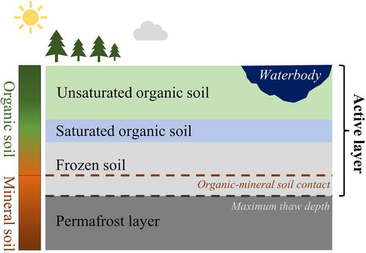
Permafrost is a key element of the cryosphere, and is defined as “cryotic ground” (soil or rock) that remains at 0°C for two or more consecutive years. Across the northern hemisphere, permafrost underlies an estimated 25% (15 million km²) of the periglacial landscape [1]. The soil layer above the permafrost which thaws and freezes on an annual basis is referred to as Active Layer Thickness (ALT; [2]; Figure 1), and is an area where several essential hydrological, biological, and chemical processes take place [3]. This is because the frozen permafrost layer below is impermeable, resulting in wet conditions, slow decomposition rates, and the accumulation of large organic carbon stores above [4]. ALT, or the maximum thaw depth of this layer, is a critical variable to monitor since it corresponds to the stability and thermal state of the permafrost layer [5]. When permafrost degrades (i.e., thaws) from changing environmental conditions, the active layer extends further into the upper portion of frozen ground. Changes to the thermal state of the ground, and accordingly the evolution of ALT, can result in permafrost layer degradation and significant impacts on terrestrial ecosystem processes [6]. These impacts on the sensitive and vulnerable permafrost layer may have significant consequences, both for local communities living on permafrost [7], as well as the global society [8].

Figure 1.

Conceptual diagram of the active layer in permafrost regions.

Important variables controlling the seasonal fluctuations and thickness of the active layer include hydrology, soil, vegetation, topography, ecotype, and climatological parameters, as well as anthropogenic activities [2, 9]. In particular, air temperatures and their inter- and intra-annual amplitudes exert a strong control on ALT, especially during the thaw season [10]. As air temperatures become warmer, the seasonal duration and depth of thawing becomes more pronounced. This makes permafrost one of the elements of the Earth system most reactive to climate change [11]. Hence why global warming is of such concern for permafrost loss and deepening of the ALT, as changes to ALT may have profound impacts on polar region hydrology and biogeochemical processes [12]. With the latter, permafrost degradation has the potential to release large stores of carbon dioxide (CO²) and methane (CH⁴; [13, 14]). This release may further amplify surface warming at a global scale, resulting in what’s referred to as the permafrost carbon feedback (PCF; [15, 16]). Recent research shows that the Arctic has warmed nearly four times the global average [17], thus the PCF and its associated mechanisms require improved understanding, measurements, and modeling in the face of climate change [18].

1.2 Remote sensing of active layer thickness

Generating regional maps of ALT is challenging, since ALT is temporally and spatially variable and reflective of the landscape’s heterogeneous hydro-ecological conditions (e.g., snow cover, moisture, vegetation, etc.; [19]). Local scale in situ methods, including ground penetrating radar (GPR), geophysical surveys and conventional human-based sampling (e.g., point-based field measurements from manual frost/thaw probing with metal rods), are proven and effective techniques for determining subsurface permafrost depth [20]. However, these methods are labor intensive, time-consuming, expensive to conduct, and therefore inefficient and not reasonably scalable over large spatial extents, especially across the very remote and inaccessible regions of the Arctic tundra. On the other hand, RS measurements, such as from EO satellite missions, offer a desirable alternative to in situ methods [21]. This is because RS methods are scalable over wide coverages, cost-effective, repeatable, and non-invasive [22].

Several studies have successfully demonstrated the effectiveness of RS (both aerial and satellite) for local-scale ALT estimation and mapping [23], although few have done so over large spatial extents of the northern permafrost region and simultaneously at high resolutions. A number of studies have used optical and/or hyperspectral imaging to map ALT [24, 25, 26], whereby retrieval of vegetation coverage is used to investigate ALT conditions. The Normalized Difference Vegetation Index (NDVI) is a well-established technique for understanding ALT with optical RS data. This is because ALT and NDVI are negatively correlated, with greater vegetation coverages (i.e., biomass) resulting in a shallower active layer [27]. Hence, NDVI is often considered as a predictor (i.e., driver) of ALT [28, 29].

Synthetic Aperture Radar (SAR) RS has also become very popular for mapping ALT. This is because the microwaves emitted by a SAR can penetrate vegetation canopies and soil surfaces, and are sensitive to subsurface conditions [30]. These conditions, such as soil organic carbon and moisture, can be used as a proxy for improved inference of ALT [21]. For example, Widhalm et al. [31] demonstrated the interrelations between X-band SAR backscatter and land cover conditions for modeling ALT, with results indicating a better performance than the NDVI variable. Interferometric SAR (InSAR) techniques in particular have proven effective for ALT estimation and monitoring [32]. The InSAR technique relies on both the phase and amplitude information contained in the SAR signal, acquired from a pair (or more) of multi-temporal SAR images [33]. By comparing the timing of the radar return between each image, the distance between the sensor and ground can be quantified. This information is used to infer permafrost conditions, since changes to the vertical distribution of pore water in the active layer is related to InSAR measured subsidence, and thus ALT [34].

1.3 Cloud-based geospatial analysis with Google Earth Engine

The availability of datasets extracted from various RS sources is ever increasing. Rapid technological advancements have resulted in an unprecedented archive of EO data, which is continuously growing in velocity, volume, and variety [35]. This proliferation of data is referred to as “big data,” which is not easily stored or processed using conventional desktop-based resources. Several cloud-based processing platforms have been developed that enable geospatial analysis [36], evidently solving the challenge of big data processing. Most prominent and widely used is Google Earth Engine (GEE), a cloud-based platform that facilitates the analysis of RS data over large spatial extents, by leveraging Google’s infrastructure [37]. Since its release in 2010, the literature on GEE has grown exponentially, showing a wide range of vital applications including agriculture [38], wetlands [39], forests [40], and bathymetry [41], to name a few. GEE is free-to-use, and houses a number of EO datasets of various spatial and temporal resolutions, such as the popular Sentinel-1 and -2, Landsat, and MODIS archives.

Google Earth Engine (GEE) also provides access to numerous advanced ML algorithms and high-speed parallel processing [42], making the mapping and monitoring of environmental variables at local to global scales realizable. The built-in ML capabilities of GEE are user friendly, and allow for solving tasks such as supervised classification, unsupervised classification, and continuous regression problems [43]. Popular ML algorithms on GEE include Classification and Regression Trees (CART), Random Forest, and Support Vector Machine (SVM; [44]). These aforementioned algorithms represent some of the prominent ML techniques that have helped revolution EO, by helping process large and diverse datasets and determining relationships between spectral measurements and environmental phenomenon [45].

2. Materials and methods

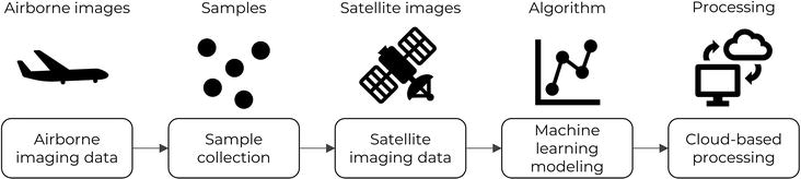
This case study leveraged airborne and satellite RS, ML modeling, and cloud-based processing to estimate large-scale ALT. The general methodology is presented in Figure 2. The following sections detail each component, followed by the results of the study.

Figure 2.

Overall methodology used in this case study for ALT mapping.

2.1 Study area

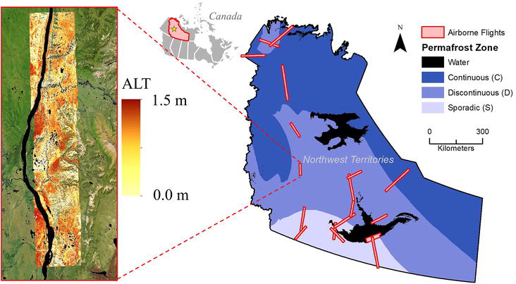
Active layer thickness (ALT) modeling and mapping was conducted across mainland Northwest Territories (NWT), Canada, covering an area of 114,000 km². Permafrost is found throughout all of the region. However, it is more common, thicker, and colder in the northern regions. This is represented by the three distinct permafrost zones which the NWT falls within: sporadic, discontinuous, and continuous. These zones are shown in Figure 3, along with the airborne RS data swaths which are described in the forthcoming sections. Research is showing that permafrost conditions across the NWT are changing, with main drivers being increased air temperatures and changes to precipitation [46].

Figure 3.

Location of the study area, NWT, Canada. Extent of ALT measurements collected by NASA airborne flights during the ABoVE campaign are shown in red.

2.2 Airborne remote sensing data

Active layer thickness (ALT) measurements used for the development, optimization, and evaluation of a ML model were acquired via active airborne SAR imaging, by Chen et al. [47]. These data were collected during the 2017 NASA Arctic Boreal Vulnerability Experiment (ABoVE) airborne campaign, and therefore represent 2017 conditions. The ABoVE program, started in 2015, is a terrestrial ecology program researching environmental change across Alaska and Western Canada using RS [48]. The ALT profiles were retrieved using joint L- and P-band SAR sensors, from NASA’s Uninhabited Aerial Vehicle Synthetic Aperture Radar (UAVSAR) and Airborne Microwave Observatory of Subcanopy and Subsurface (AirMOSS) SARs. As seen in Figure 3, 18 flight paths were conducted over the NWT, all of which were leveraged in this study. These ALT profiles have been independently validated by Parsekian et al. [49], and show good estimation compared to in situ GPR measurements.

2.3 Satellite earth observation data

The airborne RS data were upscaled to satellite EO data, since the latter are well-suited for regional mapping applications. All EO data were processed using GEE’s JavaScript application programming interface (API). EO image sources included multi-frequency SAR, from the C-band Sentinel-1 and L-band ALOS PALSAR satellites, and electro-optical imagery from Landsat-8. These EO datasets were selected since SAR can penetrate vegetation and soil surfaces and interact with sub-surface hydrological conditions [33], and Landsat-8 supplies both reflectance and thermal energy measurements which can help differentiate frozen from unfrozen ground [50]. EO image preprocessing followed that of Merchant et al. [39], and included fundamental steps such as speckle filtering and orthorectification of SAR, and cloud-masking of Landsat-8 imagery. High-resolution topographic imagery from the ArcticDEM project was also included in the modeling pipeline.

A time-series of images were collected for the SAR and electro-optical datasets, for the period of May-to-September 2017. These dates and range matched the airborne imaging acquisitions. The time-series for each EO source were then composed using a variety of aggregation functions in GEE (i.e., statistical descriptors; [51]), including mean, median, minimum, maximum, standard deviation, variance, and coefficient of variation. Each EO band and indice/variable were subject to these statistical functions, except for the time-static ArcticDEM variables. The list of satellite based EO variables used to model ALT across the NWT is found in Table 1.

EO source	Variable	Description	Statistical descriptors
Sentinel-1	σ°VV, σ°VH	C-band linear backscatter	Mean, median, minimum, maximum, standard deviation, coefficient of variation, variance
	VV/VH	C-band cross-pol ratio
ALOS PALSAR	σ°HH, σ°HV	L-band linear backscatter
	HH/HV	L-band cross-pol ratio
Landsat-8	Blue, Green, Red, NIR, SWIR1, SWIR2	Surface reflectance bands
	NDVI, NDWI	Normalized difference vegetation index and water index
	LST	Land surface temperature
	Albedo	Surface light fraction
ArcticDEM	Elevation, slope, aspect	Topographic variables	N/A
	TPI	Topographic position index

Table 1.

Satellite EO variables used for ALT estimation modeling. A total of 116 variables were collected.

2.4 Machine learning modeling

A ML approach was used to upscale the airborne ALT measurements to satellite observations. A Random Forest algorithm was chosen for this task, as it has shown to be robust and accurate for a variety of RS regression problems with GEE [52]. Moreover, it tends to handle non-linear and multidimensional geospatial data very well [53]. Random Forest is an ensemble ML algorithm that constructs multiple decision trees on random subsets of data, which then merges their predictions [54]. This improves regression performance and reduces model overfitting. Random forest has several hyperparameters that must be set in GEE. In order to optimize these values, a subset of ALT validation samples (which are described later) were used to tune each hyperparameter using the Scikit-learn and GridSearchCV packages in Python. The tuning process used the k-fold statistical cross-validation method [55]. This method randomly divides the samples into k-groups (k = 5 was used) and then trains the model using k-1 folds. The ensuing model is then validated with the remaining samples.

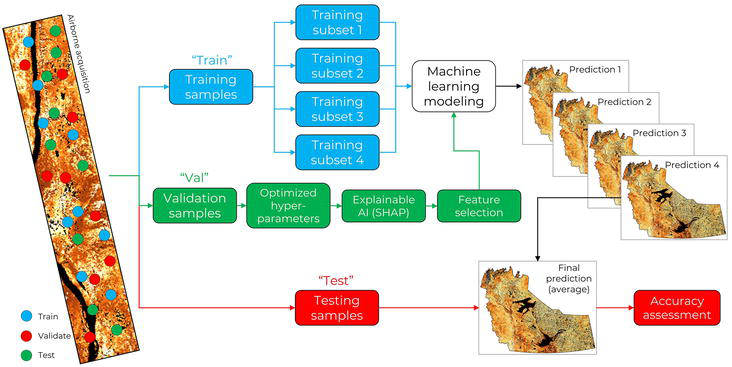
The steps taken to train, validate (i.e., optimize), and test the ML modeling are shown in Figure 4. The first step involved sampling the airborne ALT profiles. A random stratification sampling approach was used for this. Two thousand five hundred randomly generated samples were first created within each 10 cm ALT bin, which ranged from 0 to 150 cm depth (e.g., 0 to 10 cm bin, 10 to 20 cm bin, and so on). This resulted in 37,500 sampling points, which was repeated four times to obtain four subsets of model training data, and then another two times to obtain model validation and testing data. The total number of sampling points is presented in Table 2. The training data subsets were used to train four separate ML models, with the final prediction result being the average ALT value. The validation samples were used to determine optimal hyperparameters for this modeling, in addition to performing a feature selection analysis, whereas the testing samples were used solely for final accuracy assessment.

Figure 4.

Workflow for ML modeling. Blue: Data used for training. Green: Data used for validation. Red: Data used for testing.

Variable	Description	Number of samples
Training	Model 1	37,500
	Model 2	37,500
	Model 3	37,500
	Model 4	37,500
Validation		37,500
Testing		37,500
Total		225,000

Table 2.

Samples collected from airborne ALT profiles used to train, validate, and test the ML modeling.

2.5 Feature selection and model interpretation using explainable AI

Explainable AI (XAI) refers to a set of approaches used to explain and interpret ML models [56]. From these, the Shapley additive explanations (SHAP) algorithm was chosen to interpret the ML modeling of ALT [57]. SHAP is a state-of-the-art explainable AI (EAI) method, which can improve model transparency by revealing feature importance [58]. The algorithm borrows from cooperative game theory, in which the Shapley values quantify the additive, magnitudinal contribution of all variables to a model’s prediction. Hence, SHAP was used to identify and rank the contributions of all 116 EO variables using the validation samples (Table 2), in order to support a feature selection process. The 30 most important EO features identified by the SHAP algorithm were chosen as final inputs to the Random Forest modeling.

2.6 Model performance assessment

Several statistical metrics were used to assess ML model performance, including coefficient of determination (R²), room mean square error (RMSE), mean absolute error (MAE), mean square error (MSE), mean bias error (MBE), and relative absolute error (RAE):

$${\text{R}}^2=\frac{{\left({\displaystyle {\sum }_{i=1}^n\left(x_i-\overline{x}\right)\left(y_i-\overline{y}\right)}\right)}^2}{{\displaystyle {\sum }_{i=1}^n\left(x_i-\overline{x}\right)}{\displaystyle {\sum }_{i=1}^n{\left(y_i-\overline{y}\right)}^2}}$$E1

$$\text{RMSE}=\sqrt{\frac{1}{n}{\displaystyle {\sum }_{i=1}^n{\left(y_i-x_i\right)}^2}}$$E2

$$MAE=\frac{1}{n}{\displaystyle \sum _{i=1}^n\left|y_i-x_i\right|}$$E3

$$MSE=\frac{1}{n}{\displaystyle \sum _{i=1}^n{\left(y_i-x_i\right)}^2}$$E4

$$MBE=\frac{1}{n}{\displaystyle \sum _{i=1}^n\left(x_i-y_i\right)}$$E5

$$RAE=\frac{{\displaystyle {\sum }_{i=1}^n\left|y_i-x_i\right|}}{{\displaystyle {\sum }_{i=1}^n\left|x_i-\overline{x}\right|}}$$E6

where $x_i$ is the measured ALT value, $y_i$ is the predicted (i.e., modeled) ALT value, $\overline{x}$ is the mean of the measured ALT, $\overline{y}$ is the mean of the predicted ALT, and n is the total of $x$ and $y$. Model performance is best when R² is high, MBE is zero, and the remaining metrics are smaller [59].

3. Study results and discussion

3.1 Model tuning results

The ML tuning process, which took place prior to model training and application on GEE and using the subset of validation samples, resulted in a set of optimal Random Forest hyperparameters. The optimized hyperparameters, presented in Table 3, were selected based on the best model performance from the k-fold cross-validation procedure. The achieved R² from the cross-validation process was 0.432.

Hyperparameter	Values assessed	Optimal value
‘n_estimators’	[25, 50, 75, 100]	100
‘max_depth’	[None, 10, 20, 30]	None
‘min_samples_split’	[2, 5, 10, 15]	2
‘min_samples_leaf’	[1, 2, 4, 8]	2

Table 3.

Optimal Random Forest hyperparameter settings identified by the cross-validation procedure.

3.2 Explainable AI results

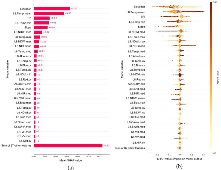
The results of the SHAP XAI analysis are presented in Figure 5, which includes both global (5a) and local (5b) feature importance plots. In both plots, only the top 30 (of 116) features are displayed, and are ordered by decreasing model importance. This is because the larger the SHAP value, the greater the contribution. These 30 features were selected as inputs to the ML modeling on GEE.

Figure 5.

(a) Global feature importance plot, displaying the mean absolute SHAP values, and (b) local feature importance plot, displayed using a SHAP beeswarm summary plot.

The global plot represents the mean SHAP value for each EO variable, which is quantified using all samples and therefore represents the average impact on model predictions. It is considered a quick and easily interpretable representation of SHAP results. This figure indicates that elevation, Landsat-8 (L8) mean and minimum LST, TPI, and slope are the five most important features explaining ALT variability.

The average global SHAP plot seen in Figure 5a is straightforward, however it does omit important information on variable contributions, such as the influence (i.e., direction) of samples on model construction. Hence, the summary plot is presented in Figure 5b, which combines feature importance and effects. Every point in the summary plot is a SHAP value for a single instance of a single EO variable. The values indicate the probability of different predicted ALT depths, based on the positive or negative correlation to ALT. For example, examination of this plot shows that low elevations, low topographic positions, and low slopes have a strong association with deeper ALTs. Deeper ALTs are also associated with warmer LSTs (both average and minimum temperatures). These findings generally align with the literature, in terms of the linkages between topography, temperatures, and permafrost [60].

3.3 Earth observation variable analysis

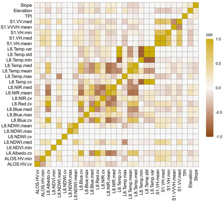
The most important EO variables, defined by the SHAP algorithm, were further analysed prior to ML modeling on GEE. In Figure 6, a correlation matrix shows the relationship between the 30 most important EO variables. Some variables showed strong correlations, such as between temperature and reflectance variables from L8. However, beyond these, most variables were not strongly correlated. This is important to note, because ML models tend to perform better when input variables are non-redundant, and multicollinearity (i.e., near-linear dependencies) is minimized [61].

Figure 6.

Correlation matrix showing the relationship between the 30 most important EO variables.

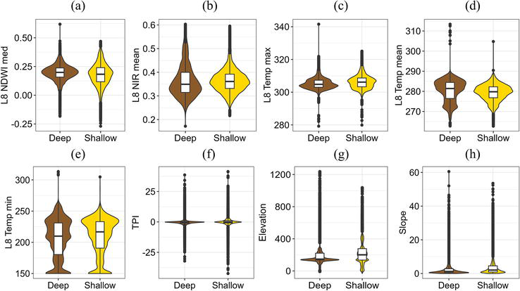
Violin plots were also used to visualize the distribution and summary statistics of the 10 most important EO variables. In Figure 7, these plots were generated for shallow (0 to 0.75 m) and deep (0.75 to 1.5 m) ALTs, thus providing additional insight into the information captured by EO satellites. In particular, it can be seen that ALT characterization is relatively challenging for any single EO variable, which suggests that a multi-source fusion approach (i.e., SAR, optical, topography, etc.) is necessary for ALT estimation and mapping.

Figure 7.

Violin plots showing the distribution of pixels for the 10 most important EO variables. The plots show the dataset distribution and summaries by ALT depth, whereby “deep” corresponds to 0–0.75 m depths, and “shallow” corresponds to 0.75–1.5 m depths.

3.4 Active layer thickness modeling results

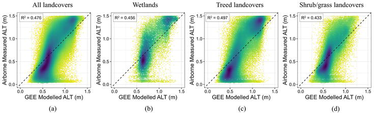
Following the tuning of hyperparameters and selection of important features, ML modeling of ALT was then implemented on the GEE. Statistical evaluation of the optimized ML model is found in Table 4. Model performance was also assessed by ecosystem type (e.g., wetlands) and vegetation (e.g., treed or shrub/grassland landcovers) based on the North American Land Change Monitoring (NALCM; [62]) landcover dataset. The ML model achieved an R² of 0.476 and RMSE of 0.313 m when evaluated across all landcovers. This performance was slightly weaker in wetland ecosystems (R² of 0.456 and RMSE of 0.299 m) and in lower biomass areas with grassy/shrub coverage (R² of 0.433 and RMSE of 0.295 m), however it was stronger in treed ecosystems (R² of 0.497 and RMSE of 0.659 m). With wetlands, saturated conditions enhance heat transfer to layers below [63], resulting in deeper permafrost depths that may be more challenging to model with EO. In contrast, forested ecosystems provide canopy shading properties that inhibit radiation-induced thaw [64], leading to shallower ALT. These characteristics have been shown to relate strongly to EO data, such as those from optical sensors (e.g., NDVI; [27]).

Landcover	R^2	MAE	MSE	RMSE	RAE	MBE
All	0.476	0.251	0.098	0.313	0.675	−0.003
Wetlands	0.456	0.234	0.089	0.299	0.678	0.002
Treed	0.497	0.264	0.106	0.327	0.659	−0.008
Grass/shrub	0.433	0.234	0.087	0.295	0.708	−0.0003

Table 4.

Performance evaluation of the ML model.

Scatterplots are presented in Figure 8 for additional visualization of model performance, which compares the airborne measured ALT to the ML predicted ALT. In general, shallower depths were better predicted than deeper depths, especially in wetlands which had deep ALTs.

Figure 8.

Scatterplots of ALT predicted using ML modeling on GEE.

3.5 Active layer thickness map of the Northwest Territories

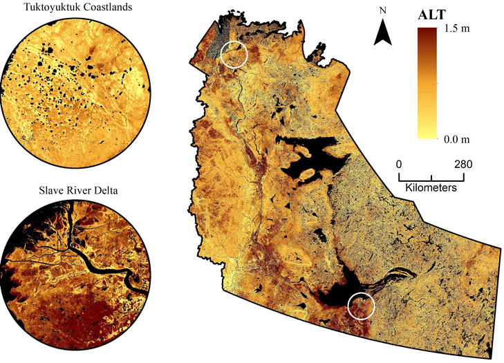
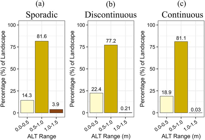
The cloud-computing resources provided by GEE were used to scale the ML predictions across mainland NWT, covering an area of 114,000 km². The final results of the modeling are presented in the Figure 9 map. Two areas are highlighted in this map, the Slave River Delta and the Tuktoyaktuk Coastlands. The former is a unique area in southern NWT consisting of vast wetland ecosystems with deep ALTs [66], whereas the latter is in the ice-rich high-latitudes where permafrost tends to be thicker and closer to the surface [67]. For example, based on the modeling outputs, the sporadic permafrost zone of the NWT was found to have the highest percentage of deep ALTs (3.9%; Figure 10), whereas the discontinuous and continuous zones (i.e., those in the higher latitudes) had the highest percentage of shallow ALTs, respectively (i.e., thick permafrost close to the surface; 22.4 and 18.9%).

Figure 9.

ALT map of the NWT produced using ML on GEE. Water bodies were masked using data from the Global Surface Water Dynamics (GSWD; [65]) project for the year 2017.

Figure 10.

Summary of ALT depths by permafrost zone across the NWT.

3.6 Advantages of cloud-based processing

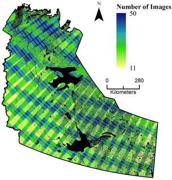
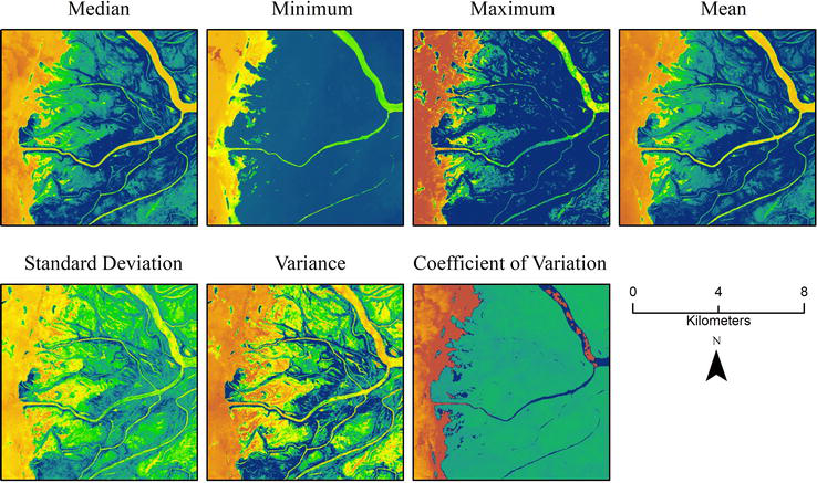
Advanced geotechnologies were leveraged in this case study for ALT mapping across a rapidly changing landscape in Canada’s Arctic region. GEE’s computational resources and rich catalog of EO data, of which is Petabytes in scale, enabled the efficient access, preprocessing, and analysis of thousands of multi-source satellite images (Figure 11). In particular, dense time-series of RS big data were rapidly reduced (i.e., aggregated) into ready-to-analyse composites using an array of statistical functions (e.g., median, mean, etc.; Figure 12). Thus, the use of GEE removed the need for powerful and expensive local computing power (i.e., high-performance computing; HCP), which is otherwise necessary for scaling high-resolution predictions over large areas with RS big data [35]. This study now joins a dense collection of literature demonstrating the large-scale modeling capabilities of GEE for environmental applications and information generation over permafrost rich landscapes [33, 68, 69, 70, 71]. As such, the use of GEE, along with other cloud-based geospatial platforms (e.g., Microsoft Azure, Amazon Web Services, etc.), is a continuously emerging trend in the field of RS and EO [72].

Figure 11.

Number of Landsat-8 satellite images processed over the study area for ALT estimation.

Figure 12.

Visual example of time-series statistical descriptors for the NDVI variable, over the Slave River Delta, NWT.

3.7 Implications for permafrost region science

Permafrost underlies much of the high-latitudes, and consequently it interacts with numerous systems including climate and human settlements [73], to name a few. Having the ability to map permafrost-related characteristics at high spatial resolutions, such as the ALT phenomenon, is important for better understanding the impacts on these and other critical systems [74]. This importance is magnified due to the accelerated warming of northern Arctic regions, which is stimulating permafrost degradation [22]. For example, thawing of permafrost can induce slope instabilities [75] and destroy valuable infrastructure [7], while at the same time altering soil hydrology, nutrient, and microbial properties that impact vegetation [76]. Hence, there is a need for improved knowledge on the spatial distribution and characterization of the permafrost active layer, in order to support monitoring efforts and better understand the impact of a changing climate. The ALT map produced in this case study helps address these needs, by potentially serving as an essential input to climate and carbon storage models, land use planning processes, and baseline ecosystem analyses. Hence why many aspects of permafrost research require high-resolution spatial distribution knowledge on variables such as ALT, and the associated seasonal freezing patterns [19].

4. Conclusions

This chapter has explored the use of new EO technologies, with a particular focus on geospatial “big data” analysis with cloud-computing. By presenting a case study on the mapping of ALT, it has been demonstrated that these emerging technologies can be used to estimate challenging and heterogenous environmental variables, at scale. Analyzing such enormous time-series stacks of EO data was once a near-impossible task using conventional RS methods, and only reserved for those with super-computing resources. However, breakthroughs in cloud processing platforms, such as the GEE, have helped the RS community overcome challenges related to access, processing, and storage. The results of this case study highlight the capabilities of innovative EO technologies for permafrost environment mapping, by leveraging new RS sensors, cloud-processing, and ML to estimate a climatically significant variable, the ALT.

References

1.Zhang T, Heginbottom JA, Barry RG, Brown J. Further statistics on the distribution of permafrost and ground ice in the northern hemisphere. Polar Geography. 2000;24:126-131
2.Luo D, Wu Q , Jin H, Marchenko SS, Lü L, Gao S. Recent changes in the active layer thickness across the northern hemisphere. Environment and Earth Science. 2016;75:555
3.Throckmorton H, Newman B, Heikoop J, et al. Active layer hydrology in an Arctic tundra ecosystem: Quantifying water sources and cycling using water stable isotopes. Hydrological Processes. 2016;30:4972-4986
5.Smith S, O’Neill H, Isaksen K, Noetzli J, Romanovsky V. The changing thermal state of permafrost. Nature Reviews Earth and Environment. 2022;3:10-23
6.Li G, Zhang M, Pei W, Melnikov A, Khristoforov I, Li R, et al. Permafrost extent and active layer thickness variation in the northern hemisphere from 1969 to 2018. Science of the Total Environment. 2022;804:150182
7.Hjort J, Streletskiy D, Doré G, Wu Q , Bjella K, Luoto M. Impacts of permafrost degradation on infrastructure. Nature Reviews Earth and Environment. 2022;24:3-1
8.Schuur EAG, Mack MC. Ecological response to permafrost thaw and consequences for local and global ecosystem services. Annual Review of Ecology, Evolution, and Systematics. 2018;49:279-301
9.Fisher JP, Estop-Aragonés C, Thierry A, Charman DJ, Wolfe SA, Hartley IP, et al. The influence of vegetation and soil characteristics on active-layer thickness of permafrost soils in boreal forest. Global Change Biology. 2016;22:3127-3140
10.Wu Q , Hou Y, Yun H, Liu Y. Changes in active-layer thickness and near-surface permafrost between 2002 and 2012 in alpine ecosystems, Qinghai-Xizang (Tibet) plateau, China. Global and Planetary Change. 2015;124:149-155
11.Chadburn S, Burke E, Cox P, Friedlingstein P, Hugelius G, Westermann S. An observation-based constraint on permafrost loss as a function of global warming. Nature Climate Change. 2017;7:340-344
12.Walvoord MA, Kurylyk BL. Hydrologic impacts of thawing permafrost—A review. Vadose Zone Journal. 2016;15:1-20
13.Chen L, Liang J, Qin S, Liu L, Fang K, Xu Y, et al. Determinants of carbon release from the active layer and permafrost deposits on the Tibetan plateau. Nature Communications. 2016;7:13046
14.Schaefer K, Zhang T, Bruhwiler L, Barrett AP, Fe RAE, Ju NZHANGIG, et al. Amount and timing of permafrost carbon release in response to climate warming. Chemical and Physical Meteorology. 2011;63:165-180
15.Schaefer K, Lantuit H, Romanovsky VE, Schuur EAG, Witt R. The impact of the permafrost carbon feedback on global climate. Environmental Research Letters. 2014;9:9
16.Miner K, Turetsky M, Malina E, Bartsch A, Tamminen J, McGuire AD, et al. Permafrost carbon emissions in a changing Arctic. Nature Reviews Earth and Environment. 2022;3:55-67
17.Rantanen M, Karpechko AY, Lipponen A, Nordling K, Hyvärinen O, Ruosteenoja K, et al. The Arctic has warmed nearly four times faster than the globe since 1979. Communications Earth & Environment. 2022;3:168
18.You Q , Cai Z, Pepin N, et al. Warming amplification over the Arctic pole and third pole: Trends, mechanisms and consequences. Earth-Science Reviews. 2021;217:103625
19.Dobiński W. Permafrost active layer. Earth-Science Reviews. 2020;208:103301
20.Sudakova M, Sadurtdinov M, Skvortsov A, Tsarev A, Malkova G, Molokitina N, et al. Using ground penetrating radar for permafrost monitoring from 2015-2017 at calm sites in the Pechora river delta. Remote Sensing. 2021;13:3271
21.Yi Y, Kimball JS, Chen RH, Moghaddam M, Reichle RH, Mishra U, et al. Characterizing permafrost active layer dynamics and sensitivity to landscape spatial heterogeneity in Alaska. The Cryosphere. 2018;12:145-161
22.Jorgenson MT, Grosse G. Remote sensing of landscape change in permafrost regions. Permafrost and Periglacial Processes. 2016;27:324-338
23.Philipp M, Dietz A, Buchelt S, Kuenzer C. Trends in satellite earth observation for permafrost related analyses—A review. Remote Sensing. 2021;13:1217
24.Pastick N, Jorgenson M, Wylie B, Minsley B, Ji L, Walvoord M, et al. Extending airborne electromagnetic surveys for regional active layer and permafrost mapping with remote sensing and ancillary data, Yukon flats ecoregion, Central Alaska. Permafrost and Periglacial Processes. 2013;24:184-199
25.Cao H, Gao B, Gong T, Wang B. Analyzing changes in frozen soil in the source region of the yellow river using the Modis land surface temperature products. Remote Sensing. 2021;13:180
26.Zhang C, Douglas TA, Anderson JE. Modeling and mapping permafrost active layer thickness using field measurements and remote sensing techniques. International Journal of Applied Earth Observation and Geoinformation. 2021;102:102455
27.Luo D, Liu L, Jin H, Wang X, Chen F. Characteristics of ground surface temperature at Chalaping in the source area of the yellow river, northeastern Tibetan plateau. Agricultural and Forest Meteorology. 2020;281:107819
28.Xu X, Wu Q. Active layer thickness variation on the Qinghai-Tibetan plateau: Historical and projected trends. Journal of Geophysical Research: Atmospheres. 2021;126:e2021JD034841
29.Zhan D, Li M, Xiao Y, Man H, Zang S. Spatial differentiation and influencing factors of active layer thickness in the Da Hinggan Ling prefecture. Frontiers in Earth Science. 2023;10:1066662
30.Merchant M, Adams J, Berg A, Baltzer J, Quinton W, Chasmer L. Contributions of C-band SAR data and polarimetric decompositions to subarctic boreal peatland mapping. IEEE Journal of Selected Topics in Applied Earth Observations and Remote Sensing. 2017;10:1467-1482
31.Widhalm B, Bartsch A, Leibman M, Khomutov A. Active-layer thickness estimation from X-band SAR backscatter intensity. The Cryosphere. 2017;11:483-496
32.Wang C, Zhang Z, Zhang H, Zhang B, Tang Y, Wu Q. Active layer thickness retrieval of Qinghai-Tibet permafrost using the TerraSAR-X InSAR technique. IEEE Journal of Selected Topics in Applied Earth Observations and Remote Sensing. 2018;11:4403-4413
33.Merchant M, Obadia M, Brisco B, Devries B, Berg A. Applying machine learning and time-series analysis on Sentinel-1A SAR/InSAR for characterizing Arctic tundra hydro-ecological conditions. Remote Sensing. 2022;14:1123
34.Zhang X, Zhang H, Wang C, Tang Y, Zhang B, Wu F, et al. Active layer thickness retrieval over the Qinghai-Tibet plateau using Sentinel-1 multitemporal InSAR monitored permafrost subsidence and temporal-spatial multilayer soil moisture data. IEEE Access. 2020;8:84336-84351
35.Ma Y, Wu H, Wang L, Huang B, Ranjan R, Zomaya A, et al. Remote sensing big data computing: Challenges and opportunities. Future Generation Computer Systems. 2015;51:47-60
36.Gomes VCF, Queiroz GR, Ferreira KR. An overview of platforms for big earth observation data management and analysis. Remote Sensing. 2020;12:1253
37.Tamiminia H, Salehi B, Mahdianpari M, Quackenbush L, Adeli S, Brisco B. Google Earth Engine for geo-big data applications: A meta-analysis and systematic review. ISPRS Journal of Photogrammetry and Remote Sensing. 2020;164:152-170
38.Phalke AR, Özdoğan M, Thenkabail PS, Erickson T, Gorelick N, Yadav K, et al. Mapping croplands of Europe, Middle East, Russia, and Central Asia using Landsat, Random forest, and Google Earth Engine. ISPRS Journal of Photogrammetry and Remote Sensing. 2020;167:104-122
39.Merchant M, Brisco B, Mahdianpari M, Bourgeau-Chavez L, Murnaghan K, DeVries B, et al. Leveraging Google Earth Engine cloud computing for large-scale Arctic wetland mapping. International Journal of Applied Earth Observation and Geoinformation. 2023;125:103589
40.Jahromi M, Zolghadr-Asli B, Pourghasemi H, Alavipanah S. Google Earth Engine and its application in forest sciences. In: Spatial Modeling in Forest Resources Management: Rural Livelihood and Sustainable Development. New York City, USA: Springer; 2021. pp. 629-649
41.Merchant MA. Modelling inland Arctic bathymetry from space using cloud-based machine learning and Sentinel-2. Advances in Space Research. 2023;72:4256-4271
42.Yang L, Driscol J, Sarigai S, Wu Q , Chen H, Lippitt CD. Google Earth Engine and artificial intelligence (AI): A comprehensive review. Remote Sensing. 2022;14:1-110
43.Gorelick N, Hancher M, Dixon M, Ilyushchenko S, Thau D, Moore R. Google Earth Engine: Planetary-scale geospatial analysis for everyone. Remote Sensing of Environment. 2017;202:18-27
44.Feizizadeh B, Omarzadeh D, Kazemi Garajeh M, Lakes T, Blaschke T. Machine learning data-driven approaches for land use/cover mapping and trend analysis using Google Earth Engine. Journal of Environmental Planning and Management. 2021;66:665-697
45.Maxwell AE, Warner TA, Fang F. Implementation of machine-learning classification in remote sensing: An applied review. International Journal of Remote Sensing. 2018;39:2784-2817
46.Mamet SD, Chun KP, Kershaw GGL, Loranty MM, Peter Kershaw G. Recent increases in permafrost thaw rates and areal loss of palsas in the western northwest territories, Canada. Permafrost and Periglacial Processes. 2017;28:619-633
47.Chen H, Michaelides R, Chen J, et al. ABoVE: Active Layer Thickness from Airborne L-and P-band SAR, Alaska, 2017, Ver. 3. Oak Ridge, Tennessee, USA: ORNL DAAC; 2022
48.Miller CE, Griffith PC, Goetz SJ, et al. An overview of above airborne campaign data acquisitions and science opportunities. Environmental Research Letters. 2019;14:080201
49.Parsekian AD, Chen RH, Michaelides RJ, et al. Validation of permafrost active layer estimates from airborne SAR observations. Remote Sensing. 2021;13:2876
50.Kalinicheva SV, Shestakova AA. Using thermal remote sensing in the classification of mountain permafrost landscapes. Journal of Mountain Science. 2021;18:635-645
51.Zhang Z, Wei M, Pu D, He G, Wang G, Long T. Assessment of annual composite images obtained by google Earth Engine for urban areas mapping using random forest. Remote Sensing. 2021;13:1-19
52.Belgiu M, Dragut L. Random forest in remote sensing: A review of applications and future directions. ISPRS Journal of Photogrammetry and Remote Sensing. 2016;114:24-31
53.Merchant M, Haas C, Schroder J, Warren R, Edwards R. High-latitude wetland mapping using multidate and multisensor earth observation data: A case study in the northwest territories. Journal of Applied Remote Sensing. 2020;14:1-18
54.Breiman L. Random forests. Machine Learning. 2001;45:5-32
55.Kohavi R. A study of cross-validation and bootstrap for accuracy estimation and model selection. IJCAI. 1995;14:1137-1145
56.Minh D, Wang HX, Li YF, Nguyen TN. Explainable artificial intelligence: A comprehensive review. Artificial Intelligence Review. 2022;55:3503-3568
57.Shapley L. Value for n-person games. In: Kuhn H, Tucker A, editors. Contribution to the Theory of Games II. Princeton, NJ, USA: Princeton University Press; 1953. pp. 307-317
58.Temenos A, Temenos N, Kaselimi M, Doulamis A, Doulamis N. Interpretable deep learning framework for land use and land cover classification in remote sensing using SHAP. IEEE Geoscience and Remote Sensing Letters. 2023;20:8500105
59.Maulud DH, Abdulazeez AM. A review on linear regression comprehensive in machine learning. Journal of Applied Science and Technology Trends. 2020;1:140-147
60.Zhang Y, Touzi R, Feng W, Hong G, Lantz TC, Kokelj SV. Landscape-scale variations in near-surface soil temperature and active-layer thickness: Implications for high-resolution permafrost mapping. Permafrost and Periglacial Processes. 2021;32:627-640
61.Merchant MA, Warren RK, Edwards R, Kenyon JK. An object-based assessment of multi-wavelength SAR, optical imagery and topographical datasets for operational wetland mapping in boreal Yukon, Canada. Canadian Journal of Remote Sensing. 2019;45:308-332
62.Giri C. Remote Sensing of Land Use and Land Cover: Principles and Applications. Boca Raton, Florida, USA: CRC Press; 2012
63.Douglas TA, Turetsky MR, Koven CD. Increased rainfall stimulates permafrost thaw across a variety of interior Alaskan boreal ecosystems. NPJ Climate and Atmospheric Science. 2020;3:28
64.Maria Stuenzi S, Boike J, Cable W, Herzschuh U, Kruse S, Pestryakova LA, et al. Variability of the surface energy balance in permafrost-underlain boreal forest. Biogeosciences. 2021;18:343-365
65.Pickens AH, Hansen MC, Hancher M, Stehman SV, Tyukavina A, Potapov P, et al. Mapping and sampling to characterize global inland water dynamics from 1999 to 2018 with full Landsat time-series. Remote Sensing of Environment. 2020;243:111792
66.Zhang F, Mosaffa M, Chu T, Lindenschmidt KE. Using remote sensing data to parameterize ice jam modeling for a northern inland delta. Water (Switzerland). 2017;9:306
67.Westermann S, Duguay C, Grosse G, Kääb A. Remote sensing of permafrost and frozen ground. In: Remote Sensing of the Cryosphere. New Jersey, USA: John Wiley & Sons, Ltd.; 2015. pp. 307-344
68.Nyland KE, Gunn GE, Shiklomanov NI, Engstrom RN, Streletskiy DA. Land cover change in the lower Yenisei river using dense stacking of Landsat imagery in Google Earth Engine. Remote Sensing. 2018;10:1226
69.Pointner G, Bartsch A. Mapping arctic lake ice backscatter anomalies using Sentinel-1 time series on Google Earth Engine. Remote Sensing. 2021;13:1626
70.Qi Y, Li S, Ran Y, Wang H, Wu J, Lian X, et al. Mapping frozen ground in the Qilian mountains in 2004-2019 using Google Earth Engine cloud computing. Remote Sensing. 2021;13:1-17
71.Zakharov M, Gadal S, Kamicaityte J, Cherosov M, Troeva E. Distribution and structure analysis of mountain permafrost. Land. 2022;11:1-21
72.Loukili Y, Lakhrissi Y, Ben ASE. Geospatial big data platforms: A comprehensive review. KN Journal of Cartography and Geographic Information. 2022;72:293-308
73.Vecellio DJ, Nowotarski CJ, Frauenfeld OW. The role of permafrost in Eurasian land-atmosphere interactions. Journal of Geophysical Research: Atmospheres. 2019;124:11644-11660
74.Gruber S. Derivation and analysis of a high-resolution estimate of global permafrost zonation. The Cryosphere. 2012;6:221-233
75.Deline P, Gruber S, Amann F, et al. Ice loss from glaciers and permafrost and related slope instability in high-mountain regions. In: Snow and Ice-Related Hazards, Risks, and Disasters. Amsterdam, Netherlands: Elsevier; 2021. pp. 501-540
76.Jin XY, Jin HJ, Iwahana G, Marchenko SS, Luo DL, Li XY, et al. Impacts of climate-induced permafrost degradation on vegetation: A review. Advances in Climate Change Research. 2021;12:29-47
Written By
Michael A. Merchant and Lindsay McBlane
Submitted: 22 January 2024Reviewed: 23 January 2024Published: 16 April 2024