Constructing an Eligibility Index for the Federal Reserve Swap Line

Abstract

This study explores the eligibility criteria for swap line agreements with the Federal Reserve (Fed) by constructing a composite index that incorporates macroeconomic and U.S.-related indicators. The aim is to provide insight into the factors affecting the Fed’s decision-making process and shed light on the variables that impact a country’s eligibility for swap lines focusing on the Global Financial Crisis period and Covid-19 pandemic period. Using logistic regression model and principal component analysis, the study constructs two sub-indices: the Macroeconomic Index and the U.S. Related Index. These indices capture relevant indicators likely used in the assessment process of countries. The model’s effectiveness is tested by analyzing countries that were rejected for swap line agreements. Findings reveal that several macro-level variables and U.S.-related variables significantly explain a country’s probability of establishing a secure swap line with the Fed. Key indicators include trade volume, real GDP, international reserves, external debt, and U.S. financial claims on foreign countries. The constructed composite index successfully predicts eligibility outcomes for the countries studied, demonstrating a high level of accuracy. Policy implications derived from the study highlight the importance of transparency, robust index construction, macroeconomic stability, bilateral relationships, and predictive modeling.

1. Introduction

One of the unconventional monetary policy facilities that have been in the toolkit of the central banks and monetary authorities for years is the central bank swap line agreements. Different countries have been utilizing swap line agreements for a wide range of purposes to deal with the problems occurring in times of stress as a key element of the global financial safety net [1, 2] to succeed in economic and foreign policy goals [3] to provide liquidity, and to decrease funding costs.

In today’s financial environment, swap instrument is more broadly used for the exchange of currencies, commodities such as livestock, oil, or precious metals, interest rates, and equities. The foreign exchange swap is defined in Dodd-Frank Act as a transaction that solely involves an exchange of two different currencies on a specific date at a fixed rate that is agreed upon on the inception of the contract covering the exchange; and a reverse exchange of the two currencies at a later date and at a fixed rate that is agreed upon on the inception of the contract covering the exchange.

In a simple model of central bank swap line agreement as illustrated in Figure 1, Central Bank A, which establishes swap line agreements, credits the account of Central Bank B (Foreign Central Bank) in its own books with A’s currency; in return, Central Bank B credits the account of Central Bank A in its books with an equivalent amount of B’s currency. These transactions may be interpreted as each central bank lends its currency to the counterparty. The recipient central bank commits to pay interest for the borrowed amount of foreign exchange. Central Bank B lends the foreign exchange that is borrowed from Central Bank A to eligible foreign financial institutions under its jurisdiction against high-quality collateral. In terms of the counterparty risks of central bank swap line operations, central banks that initiate the swap line agreements do not bear any risk because they do not have any relationship with foreign financial institutions that are under the jurisdiction of foreign central banks in theory. However, there is a possibility that foreign central banks might not repay their swap debt in practice.

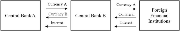
Figure 1.

Mechanism of swap line agreement.

To illustrate how the Fed implements this facility with foreign central banks, [4] provides a detailed scheme of the swap line process as following (Figure 2):

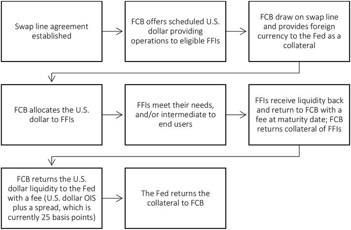
Figure 2.

From the fed to foreign financial institutions: Process of swap line. Source: Choi et al. [4]. Note: FCB: Foreign central Bank; FFI: Foreign financial institution.

Central bank swap line agreements, which have been utilized with different motives by the Federal Reserve since the 1960s, came to the fore during the Global Financial Crisis. Increasing financial stress abroad due to the panic-induced reasons has led the Fed to take additional steps to help maintain the flow of credit to U.S. households and businesses by reducing financial stresses abroad, which could pose a risk to the U.S. credit markets. The Fed approved currency swap agreements, known as swap line agreements, with several foreign central banks to relieve the burden on the U.S. dollar liquidity.

During both the global financial crisis and the Covid-19 pandemic, some countries that have requested to benefit from swap line facilities were rejected by the Fed without any further explanation. Although there is a rigid selection process behind Fed’s final decisions, neither the eligibility criteria have been disclosed to the public nor the selected countries have changed. This lack of information on the Fed’s criteria and the consistency of the selected countries encourage this study to construct a composite index of potential indicators that the Fed may have considered in the selection process of swap partners.

There is a scant literature, which aims to bring light on which factors have an impact on the selection process in swap line agreements, especially with the Fed. Although their analyses contribute to swap line agreement literature, an index aiming to combine individual indicators, which are thought to have important roles in the selection process of the Fed, will help researchers and individuals to understand the working mechanism of swap line agreements. This situation leads this study to ask the following questions:

1. What are the potential individual indicators used in the assessment of countries requesting to participate in the Fed swap line network?

2. Is it possible to construct a single index to use as a main criterion while evaluating the countries’ applications for a swap line with the Fed?

For this reason, this study aims to construct a composite Fed swap line index, covering macroeconomic and the U.S.-related indicators of countries, to give insight into the selection process of the Fed. Therefore, this study will contribute to the extant literature by combining both macroeconomic and the U.S.-related indicators to ease the interpretation process of combined indicators rather than individual indicators, facilitating communication with the public, from expert to lay and literate audiences.

The remainder of this paper is structured as follows. In the following section the historical evolution of Fed’s swap line, Fed’s decision-making process, and the impact of Fed’s swap lines on global financial stability will be discussed. In section three, the related literature will be reviewed. In section four, the details of data and methodology will be explained. In section five, how the indices are constructed will be revealed with the findings. While the sixth section will discuss the results in terms of the policy implications, in the last section the study will be concluded.

2. Evolution of Fed’s swap line and its impact on global financial stability

The Fed swap line agreements should be discussed in two different periods which have critical moments. Between 1960 and 2000, the first period covers critical decisions regarding why swap lines are required, how they operate, which central banks can participate in the swap network, etc. In this period, the U.S. and international economy, witnessed lots of historical moments such as the Great Inflation, Smithsonian Agreement, Recession of 1981–1982, Saving and Loan Crisis in the 1980s, Oil Shock of 1973–1974 and 1978–1979, and eventually the Collapse of Gold Convertibility of the Bretton Woods System. The second period is between 2001 and 2021, which witnessed historical developments such as September 11, 2001, the global financial crisis that started in the summer of 2007, and the pandemic that broke out in 2020.

In 1960s, possible current account deficits in the U.S. were on the agenda of economists and decision-makers. Actually, the U.S. had a current account surplus throughout the 1960s but trade and current account surpluses were not adequate to finance net private investment and miscellaneous spending abroad. In the same period, U.S. exports became less competitive with European and Japanese exports. After the U.S. share of world output decreased, foreign countries changed their preferences from the U.S. dollar to gold. The U.S. had two options to settle the current account balance through selling gold or accumulating the U.S. dollar liabilities for foreign countries. “The vast amount of liabilities and declined gold reserve brought along concerns regarding whether the U.S. could maintain confidence that gold price would remain fixed” [5 , p. 56]. Despite the commitment of the U.S. to keep the value of gold fixed, the economic developments caused it not to fulfill its obligation given by the Bretton Woods System. On October 20, 1960, the price of gold in the London market surpassed the committed level, $35 per ounce, and reached $40 per ounce with soared private demand for gold. This situation justified the concerns about the intervening capacity of the U.S. on the gold price and the future of the Bretton Woods System.

Increasing concerns and fluctuations on the gold price, which was committed to fixing at $35 per ounce, led the U.S. to take actions to boost confidence in the U.S. dollar and to preserve gold reserve which shrank due to the demand of foreign countries. In this regard, the Fed began consideration of utilizing foreign-exchange market operations, after nearly 39 years of inactivity, in the spring of 1961. In February 1962, the FOMC authorized the FRBNY to undertake open-market operations in foreign currencies [6]. The Fed toolkit had four different methods in the 1960s: swap lines, foreign currency-denominated bonds, called “Roosa bonds,” drawings on the U.S. reserve position in the IMF, an international organization called “gold pool” [7, 8].

The Bretton Woods System, which became operational in 1958, brought along problems to the international economic system. Impairments in the gold price and the U.S. dollar liabilities led the Fed to set up swap lines with foreign central banks and its first swap line agreement was signed with the Bank of France in March 1962 [9]. Even though this agreement was the first one in a series of agreements, including several central banks, the Fed had already had a swap agreement with the Swiss National Bank (SNB). This agreement had aimed to provide “liquidity in the U.S. dollar to support the efforts of the U.S. dollar reserve retention rather than a demand for gold by either Swiss banks or by the SNB” [10 , p. 9]. By the end of 1962, the Fed had set up lines with nine central banks in the form of standing facilities that could be drawn on request of central banks: Austria, Belgium, Canada, France, Germany, Italy, the Netherlands, Switzerland, and the United Kingdom. The amount of the Fed swap lines to each central bank was between $50 and $250 million.

In addition to these central banks, the Fed established swap line agreements with the Bank for International Settlements (BIS) in 1962, against Swiss franc, and 1965, against other European currencies (OTEUC), because of its special status of being a clearing bank for central banks. The Fed’s first swap line agreement with the BIS in 1962 was established at the request of the SNB. One of the reasons behind the SNB’s request was Swiss statutory limits on “loans” to non-Swiss banks. The Fed’s second swap line agreement with the BIS in 1965 relied on the Fed’s expansionary swap network policy for other central banks using European currencies (other than Swiss francs). Thus, the Fed reached access to other European currencies through the BIS. The size of the swap lines was increased periodically in the 1960s and 1970s. In early 1963, swap agreements totaling $900 million were outstanding on a standby basis [11]. Swap lines were generally for 3- or 6-month periods but were renewable upon mutual agreement. The FOMC renewed these initial agreements for further dates in succeeding meetings. In addition to these agreements, new swap agreements with foreign central banks came into life—the BoJ in 1964, Norges Bank, Bank of Mexico, and Danmarks Nationalbank in 1967. The Fed swap network with foreign central banks expanded, and it evolved from a small, very short-term credit facility covering $900 million in 1962 to a large, intermediate-term facility covering $11.73 billion in 1971.

The U.S. witnessed a series of the most lethal terrorist attacks in history on September 11, 2001. The terrorist attacks caused nearly three thousand lives, and a potentially serious crisis for the economy due to the impacts on financial markets. The immediate effects of the terrorist attacks were the disruption of the payments system, a one-week closure of the New York Stock Exchange (NYSE), fall in prices of U.S. stock, and the risen implied volatility of equities.

As a result of being lender of last resort in the U.S. dollar, the Fed established new swap line agreements with foreign central banks to smooth the functioning of U.S. financial markets by providing liquidity to foreign central banks whose operations in the U.S. had been disrupted by terrorist attacks. The first swap line agreement was established, on short notice, with the ECB on September 12, 2001. The swap line which had 30 days maturity, provided liquidity in the U.S. dollar to the ECB to meet the liquidity needs of European banks through national central banks of the Eurosystem. The ECB drew $20 billion on this swap line agreement.

On September 13, 2001, the Fed temporarily increased the existing swap line, $2 billion to $10 billion, with the BoC to ensure that Canadian banks could access liquidity in the U.S. dollar. The Fed’s immediate step to provide liquidity through this standing facility was welcomed, but the BoC did not draw on this swap line in 2001. The BoE was the third central bank that the Fed established a swap line with on September 14, 2001. As all of the press releases dated September 2001 regarding swap line agreements with mentioned central banks stated these swap line agreements had 30 days maturity, so they were not renewed by FOMC.

From 2001 to 2007, the Fed renewed the swap line agreements with the BoC and the Bank of Mexico, established under the North American Framework Agreement (NAFA). In addition to these swap line agreements, the Fed had to establish new ones with other central banks in an environment where the U.S. economy had substantial strains and volatility in 2007 stemming from deterioration of the subprime mortgage sector. The main purpose of swap line agreements established on the eve of the global financial crisis was to relieve the elevated pressures in short-term dollar funding markets. The FOMC authorized the Fed to establish swap line agreements for a period of up to six months with the ECB on December 6, 2007 and the SNB on December 11, 2007. Both the ECB and the SNB drew total amount of swap lines in December 2007 (Table 1).

Counterparty	Amount (millions of the U.S. dollars)
Bank of Canada*	2000
Bank of Mexico*	3000
European Central Bank	20,000
Swiss National Bank	4000

Table 1.

Swap line agreements before the global financial crisis.

*

Swap line agreement established under the North American Framework Agreement.

Existing swap line agreements with the ECB and the SNB were extended many times upon developments in the markets by the FOMC in 2008. In addition to the maturity extensions, the FOMC also increased the size of the swap line agreement with the ECB from $20 billion to $30 billion and the amount of the swap line agreement with the SNB from $4 billion to $6 billion in March 2008. In May 2008, the sizes of swap line agreements were increased to $50 billion and $12 billion, respectively. At the end of 2008, the sizes of swap line agreements with the ECB and the SNB reached $240 billion and $60 billion, respectively. Even though the Fed established swap line agreements with the ECB and the SNB at first in early 2008, in addition to existing swap line agreements with the BoC and the Bank of Mexico since 1994, its swap network expanded to meet the need for liquidity in the U.S. dollar in short-term funding markets in the third quarter of 2008. William C. Dudley, who was the manager of the system open market account, addressed the members of the FOMC about telephone conversations with his counterparts from the Norges Bank, the ECB, and the BoJ at the FOMC meeting held on September 16, 2008. The telephone conversations with his counterparts were about the need for liquidity in the U.S. dollar of local banks that were under the jurisdiction of these central banks. Upon this critical information coming from the foreign central banks, the FOMC authorized the Foreign Currency Subcommittee to establish swap line agreements with the foreign central banks as needed to address stress in money markets in their jurisdictions on September 16, 2008. Since the FOMC’s decision did not specify the amount of the agreement and which foreign central banks the swap line agreement would be made with, it was considered an open-ended authorization.

As market conditions deteriorated globally following the bankruptcy of Lehman Brothers on September 15, 2008, the Fed speeded up its expansion on swap line agreements. On September 18, 2008, the Fed announced new swap line agreements with the BoE, the BoJ, and the BoC in amounts of up to $40 billion, $60 billion, and $10 billion, respectively.

On October 13, 2008, the FOMC removed the limits on swap line agreements [12]. Following the Fed’s actions to boost swap line agreements in October 2008, the next move was establishing swap line agreements with emerging market economies (Table 2).

Counterparty	Amount (millions of the U.S. dollars)
Bank of Canada	30,000
Bank of Canada*	2000
Bank of Korea	30,000
Bank of Mexico	30,000
Bank of Mexico*	3000
Bank of England	Unlimited
Bank of Japan	Unlimited
Central Bank of Brazil	30,000
Danmarks Nationalbank	15,000
European Central Bank	Unlimited
Monetary Authority of Singapore	30,000
Norges Bank	15,000
Reserve Bank of Australia	30,000
Reserve Bank of New Zealand	15,000
Sveriges Riksbank	30,000
Swiss National Bank	Unlimited

Table 2.

Fed swap line agreements during the global financial crisis.

*

Swap line agreement established under the North American Framework Agreement.

Source: Federal Reserve Bank of New York, Treasury and Federal Reserve Foreign Exchange Operations, October–December 2008.

During the Covid-19 period, the Fed utilized temporary and standing swap line agreements on a massive scale to manage liquidity shortages abroad as the global financial crisis. While the Fed maintained the liquidity-providing operations through standing swap lines, the FOMC authorized the Fed to establish temporary swap line agreements with the BoK, the Norges Bank, the Central Bank of Brazil, the Bank of Mexico, the Danmarks Nationalbank, the MAS, the RBA, the RBNZ, and the Sveriges Riksbank on March 19, 2020 [13]. These additional swap line agreements, which would expire in September 2020, were extended through March 31, 2021 at the FOMC meeting held on July 28–29, 2020 (Table 3) [14].

Counterparty	Amount (millions of the U.S. dollars)
Bank of Canada	Unlimited
Bank of Canada*	2000
Bank of England	Unlimited
Bank of Korea	60,000
Bank of Japan	Unlimited
Central Bank of Brazil	60,000
Bank of Mexico	60,000
Bank of Mexico*	30,000
Danmarks Nationalbank	30,000
European Central Bank	Unlimited
Monetary Authority of Singapore	60,000
Norges Bank	30,000
Reserve Bank of Australia	60,000
Reserve Bank of New Zealand	30,000
Sveriges Riksbank	60,000
Swiss National Bank	Unlimited

Table 3.

Swap line agreements during the pandemic.

*

Swap line agreement established under the North American Framework Agreement.

Source: Press releases of the Board of Governors of the Federal Reserve System.

3. Literature review

Aizenman and Pasricha [15] are among the first scholars who study the factors behind the selection process of swap line agreements with emerging economies. The scholars use probit regressions to estimate the probability of being accepted for a swap agreement with the Fed and investigate four different variables, U.S. bank exposure, the share of a country in total U.S. international trade in 2007, the capital account openness of the country as of 2004 and the years since independence or 1800. They find that large U.S. banks’ exposure to selected countries, substantial U.S. trade exposure to selected countries, capital account openness, and solid credit history are the main factors in the swap line agreements established in the global financial crisis.

Ref. [16] investigate swap line agreements established with the ECB, the Fed, and the PBoC between December 2007 and October 2009. The researchers categorize countries as swap receiver (22 countries) and non-receiver (191 countries) and investigate the significance of foreign exchange reserve, nominal currency depreciation, short-term external debt, export credits, GDP, bilateral trade between the countries of swap line agreement providers on the decision process. The researchers use several methods such as seemingly unrelated, probit, Tobit regressions to estimate the relationship between the variables and being selected as a swap line agreement partner. They conclude that countries that have significant trade and financial relations with swap line provider countries secure swap line agreements with those countries.

Ref. [17] uses probit and logit models to test the relationship between currency-specific liquidity shortages and swap line agreements. The researchers selected advanced and emerging economies that experienced currency-specific shortages in the U.S. dollar, euro, Japanese yen, pound sterling, and Swiss franc in December 2008 as a sample. Results of regressions show that currency-specific shortages in euro, yen and the Swiss franc have a positive impact on the probability of securing a swap line agreement, while the relationship between the U.S. dollar shortages and swap line agreements is not significant.

Ref. [18] investigates a set of selection criteria for China’s bilateral swap agreements established between 2001 and 2013. The researchers use a simple logistic regression model to identify the determinants of swap agreements based on a gravity model with variables such as GDP, distance to Beijing, credit/GDP ratio, share of export, share of import, having a free trade agreement with China, foreign country’s direct investment into China, China’s direct investment into a foreign country, the Chinn-Ito Index for capital account openness, foreign reserve, having a sovereign default occurred between 1983 and 2010, five-year average inflation rate before the establishment of the swap, rate of the Rule of Law Index, and the rate of the Corruption Index. They find that countries’ economic sizes (nominal GDP in U.S. dollar), amount of bilateral trade, distances from Beijing, China’s capital, and having a free-trade agreement increase the likelihood of being accepted as a counterparty in the PBoC swap line agreement.

Using a probit model, Broz [19] studies both the political and financial sides of the swap line agreements and tries to find which factors might have an impact on the selection process of the Fed. The research has eight different variables that are bank exposure, GDP (% of world), liquid liabilities (% of world), bilateral trade (% of total U.S. trade), inflation (average between 1997 and 2007), reserves (% of GDP), dollar shortages, and being global financial center to estimate the impact of these variables on the selection process. As a result of regressions carried out in four different models, bank exposure, being a global financial center, reserves (in percent of world), inflation, and liquid liabilities (in percent of world) variables are found statistically significant while bilateral trade, GDP (in percent of world), and dollar shortages variables are not found statistically significant.

Ref. [20] investigated the impact of swap line agreements established by the Swiss National Bank (SNB) on stock returns using data from banks in emerging markets. The authors find that the strong response of Central and Eastern Europe bank stocks, especially local and less-well-capitalized banks, to swap lines shows that swap line agreements can impact a broader range of financial assets such as interest rate spreads, credit default swap rates, or exchange rates. Their study also shows that the structure of the banking system has a partial role in the effectiveness of international swap lines. Ref. [21] reached a similar conclusion that swap line agreements play a positive role in alleviating the international transmission of shocks to U.S. dollar funding costs, in their study focusing on the vulnerability of U.S. dollar funding.

Ref. [22] investigates the swap line agreements’ monetary policy effects from three perspectives, which are balance sheets and operations of central banks, financial markets and the transmission of monetary policy, and macroeconomic effects through investment decisions. The research shows that the swap line agreements help to ease funding pressures, the choice of investments swap line fund, the asset prices of these investments, and the stock prices of the investors.

Ref. [23] investigates swap line agreements’ effectiveness in alleviating the international liquidity stress during the euro-area sovereign debt crisis, find that the announcements of the swap line agreement have a significant effect in reducing euro-dollar foreign exchange swap spreads at the three-month maturity, but its effectiveness remains limited in easing international liquidity stresses.

Ref. [24] analyses the swap line agreements’ possible impacts on economic and financial consequences of dollar shortage with a model calibrated to the Korean experience during the pandemic and finds that swap line agreements with the Fed can reduce the negative impacts of dollar shortage shocks on domestic bank lending, investment, consumption, and domestic output.

Ref. [25] focusing on the European Central Bank (ECB) euro liquidity lines, including repo and swap lines, find that these facilities are effective in decreasing the premium of euros in foreign exchange markets in a narrow window around the announcement. Moreover, researchers put forward that these facilities can increase the use of the euro as an international currency.

In a recent study, Ref. [26] studied swap line agreements provided by different countries. By constructing an unbalanced annual panel data for emerging and developing economies for the period of 2000–2019, they test the significance of vulnerability variables -external debt, current account balance, gross foreign reserves and annual percentage change of the exchange rate-, domestic variables -real GDP growth, CPI inflation rate, fiscal primary balance and real GDP per capita-, and openness variables -net capital inflows, the sum of exports and imports of goods and services and IMF net lending-. In the group of external vulnerability variables, none of the tested variables were found statistically significant except the external debt. Among the domestic variables, only real GDP per capita is found statistically significant while in the group of openness variables, the sum of exports and imports of goods and services is found statistically significant. As a result, the researchers conclude that countries that have weak external position are more likely to establish swap line agreement, and if this country has low international reserves, she is more likely to roll over her swap line agreement.

Lastly, Ref. [27] discovered that military alliances are a key factor influencing swap line selectivity in a recent analysis of the 2020 swap lines.

4. Data & methodology

4.1 Data

The data set covers the period from 2008 to 2022 to investigate the swap lines that are opened by the Fed. In order to investigate the decision mechanism of Fed, we collected annual data of 36 countries for three different groups. According to that the first group is the countries that established a swap line with Fed. While the countries that belong to second group are known that they applied for a swap line agreement but rejected,¹ and the third group is formed with other non-receiver countries (Table 4).

Countries with Swap Line Agreements	United Kingdom, Canada, Japan, Korea, Mexico, Brazil, Denmark, Euro-area, Singapore, Norway, Australia, New Zealand, Sweden, Switzerland
Countries that were Rejected	Chile, Dominican Republic, Iceland, India, Indonesia, Peru, Poland, Turkey, South Africa
Other Non-receiver Countries	Russia, Argentina, Colombia, Dominican Republic, Panama, Paraguay, Algeria, Egypt, Morocco, Nigeria, Tunisia, China, Malaysia, Philippines, Thailand

Table 4.

Country set.

The U.S. Government Accountability Office (GAO) underlines that the FOMC accepts swap line request of countries based on the economic and financial situations, and the probability that the swap line would make an economic difference [29]. This study evaluates the country’s economic and financial eligibility through 16 initial variables in the group of macroeconomic indicators. Refs. [16, 18] suggest that the financial and trade linkages with the swap line provider countries have a positive impact on the selection process in swap line agreements, so this study uses six U.S.-related indicators for the initial analysis (Table 5).

Macro Variables	U.S.- Related Variables
Real GDP Growth (percent)	Foreign Trade of the U.S. with Foreign Countries
Fiscal Primary Balance (in percent of GDP)	Foreign Countries’ Financial Claims on the U.S. Financial Firms
Net Capital Inflows	U.S. Direct Investments into Foreign Countries
Sum of Exports and Imports of Goods and Services	Foreign Countries’ Holdings of the U.S. Treasury Securities
IMF Net Lending	U.S. Bank Exposure
Interest Rate	Annual Percentage Change of the Exchange Rate (U.S. dollar against local currency)
Money Supply
Gross National Income
Growth in Real Consumption
Stock Market Index
Real GDP (PPP) per Capita
International Reserves (incl. gold)
Current Account Balance (in percent of GDP)
External Debt (in percent of GDP)
Unemployment Rate
Consumer Price Index (percent at the end of period)

Table 5.

Variables that were used in the initial logit model.

While logistic regression does not require the error terms (residuals) to be normally distributed and homoscedasticity, the independent variables should not be too highly correlated with each other. For that reason, we test our data for multicollinearity and the null of multicollinearity is rejected for all variables. On the other hand, after identifying the significant variables, before the index construction step, data set should be tested whether it is adequate for the PCA. In this regard, Kaiser-Meyer-Olkin (KMO) Measure of Sampling Adequacy is used. The data set is found suitable for the PCA as the KMO is found higher than the minimum accepted value −0,5-.

The data set for this study is constructed by using various sources. According to that for the macrolevel variables, the data are compiled from the World Bank, International Financial Statistics (IFS) of the IMF, Balance of Payments and International Investment Position Statistics, IMF’s World Economic Outlook Database, and Central Banks’ statistics. For the U.S.-related variables, U.S. Bureau of Economic Analysis and U.S. Treasury databases are used.

4.2 Methodology

We believe that for our research question, PCA is the best-fit methodology as we try to develop a practical eligibility tool. Although there are various academic studies that aim to bring light on which factors have an impact on the selection process in swap line agreements, we believe that an index that combines individual indicators, which are thought to have significant roles in the selection process of the Fed, will help to understand the decision mechanism. In addition to that, we also benefit from the probit/logit methodology in the first step of our study.

CI aims to measure multidimensional concepts which cannot be explained by a single indicator. OECD defines CI as: “CI is formed when individual indicators are compiled into a single index, on the basis of an underlying model of the multi-dimensional concept that is being measured” [30]. As the OECD recommends, multivariate analysis is critical to comprehend the relation between individual indicators composing composite indicators. The PCA is one of the oldest and well-known methods of multivariate analysis. The main idea of PCA, which is called as dimension-reduction tool, is to reduce the dimensionality of a data set in which there are a large number of interrelated variables (P) to a much smaller number of principal components (M) while containing as much as possible of the variation present in the data set [31].

This situation reveals that this study has some limitations on the dimensions of indices and the sample of countries. This study uses 22 different indicators, 16 of which are macroeconomic indicators, to construct two sub-indices and composite indices. It is possible to say that the FOMC may use other quantitative and even qualitative indicators in the assessment process. In further studies, the data set can be expanded by adding new quantitative and qualitative indicators to construct indices. For instance, political relations with the U.S., geopolitical importance, and political stability can be included in the data set to construct another sub-index.

4.2.1 Logistic regression model

When a swap line agreement with the Fed is established, the dependent variable in the regression model takes the value of 1, and when there is not a swap line agreement with the Fed, it takes the value of 0. The probability of a swap line agreement is explained by the model as a function of explanatory factors that characterize the country’s macroeconomic situation and its financial ties to the United States. The parametric logit estimation provides a chance to determine whether the model’s explanatory variables have significant explanatory power and the capacity to predict the likelihood of potential future swap line agreements.

When a swap line is established, the dependent variable in the binomial choice model takes the value 1, and when there is not a swap line, it takes the value 0. On the right side of the model, there are indicators acting as independent variables, and the swap line variable, denoted by Y_i,t, is a dependent variable according to the model.

The logit model is derived from the simple linear regression model which takes the form [32]:

$$y_{i,t}=\alpha +\underset{i=1}{\overset{N}{\Sigma }}{\beta }_{i,t}{x}_{i,t}+{\epsilon }_{i,t}$$E1

where $y_{i,t}$ represents the probability of establishing a swap line, $x_{i,t}$ denotes the macro variables and U.S.-related variables, ${\beta }_{i,t}$ represents the coefficients of the relevant scoring functions indicators, and ${\epsilon }_{i,t}$ is the error term.

Using the logit model, this linearity problem can be solved by applying an exponential transformation as follows:

$$y_{i,t}=f\left(w_{i,t}\right)=\frac{1}{1+e^{-w}}$$E2

where $y_{i,t}$ represents the probability of establishing a swap line and $w_{i,t}=\alpha +{\Sigma }_{i=1}^N{\beta }_{i,t}{x}_{i,t}$ is the linear function of the macro variables and U.S.-related variables in Eq. 1. Performing further computations gives:

$$\mathit{ln}\frac{s_{i,t}}{1-s_{i,t}}=\alpha +\underset{i=1}{\overset{N}{\Sigma }}{\beta }_{i,t}{x}_{i,t}$$E3

where $s_{i,t}$ represents the probability of establishing a swap line at the one-year forecast horizon, $x_{i,t}$ denotes the macro variables and U.S.-related variables, ${\beta }_{i,t}$ represents the coefficients of the relevant scoring function indicators. The implicit interpretation of Eq. (3) is that the probability of establishing a swap line is linearly related to the explanatory variables multiplied by their coefficients. Subsequently, the relationship for the probability of establishing a swap line is derived and expressed using the following logit curve:

$$s_{i,t}=\frac{1}{1+e^{-{\Sigma }_{i=1}^N{\beta }_{i,t}{x}_{i,t}}}$$E4

4.2.2 PCA analysis

Composite indices aim to measure multidimensional concepts that cannot be explained by a single indicator. As composite indices have multiple variables that have different measurement units (e.g., number of swap line agreements, total size of drawing on swap lines, GDP growth rate, current account balance, etc.) the variables should be normalized to make them comparable before data aggregation step. All indicators are standardized by using the z-score method, which aims to convert indicators to a common scale with a mean of zero and standard deviations of one.

$$Z=\frac{\mathrm{X}-\mu }{\sigma }$$E5

This study utilizes the PCA to determine the weights of individual indicators to construct a composite index. In this process, the loading of rotated indicators is the first step to calculate the final weight of indicators. Following the varimax rotation of components, loadings of indicators are squared to compute the unity sum by dividing squared loadings in each component by the explained variance of the respective components. Each indicators’ squared loadings are divided by the explained variance of the respective component to compute the unity sum. Following the obtained unity sum values, component weights are computed by the explained variance of the component divided by the total variance explained by components that have eigenvalues greater than 1. As a next step, the unity sum and component weight are multiplied and the resultant is divided by summation of multiplied values to compute final weights.

Each normalized indicator is multiplied by its final weight and then aggregated into the Macro Economic Index (MEI), and the U.S. Related Index (USRI) by using the linear aggregation method.

$${\mathit{MEI}}_i=w_{\mathit{mev}1}{Y}_i^{\mathit{mev}1}+w_{\mathit{mev}2}{Y}_i^{\mathit{mev}2}+\dots$$E6

$${\mathit{\text{USRI}}}_i=w_{\mathit{\text{usrv}}1}{Y}_i^{\mathit{\text{usrv}}1}+w_{\mathit{\text{usrv}}2}{Y}_i^{\mathit{\text{usrv}}2}+\dots$$E7

where i denotes the country, and MEI and USRI capture macroeconomic indicators (mev) and the U.S.-related indicators (usrv), respectively.

As pointed out by Ref. [33], a composite index made up of a number of normalized sub-indices is recommended to be standardized after aggregation process is completed. In this regard, the MEI, and the USRI are normalized to ensure that the values of the indicators are expressed in a common scale with a mean of zero and a standard deviation of one before the last step.

$${\mathit{\text{COMPI}}}_i={\mathit{MEI}}_i+{\mathit{\text{USRI}}}_i$$E8

5. Findings

5.1 Determinants of the index according to logit model estimation

Logit model results reveal that six out of sixteen tested macro-level variables and three out of six U.S.-related variables significantly explain the probability of a country to securely establish a swap line with FED.

Table 6 presents the results of a logistic regression model where the dependent variable is a binary variable indicating whether the country has a swap line with the U.S. Federal Reserve or not. Based on the t-statistics, several explanatory variables are statistically significant at different levels of significance. Specifically, the variables that are statistically significant at the 1% level are the sum of exports and imports of goods and services, real GDP (PPP), international reserves (including gold), external debt, foreign trade of the U.S. with foreign countries, foreign countries’ financial claims on U.S. financial firms, and U.S. direct investments into foreign countries. The variables that are statistically significant at the 5% level are interest rate and unemployment rate. The adjusted R-squared value of the model is 0.537, which indicates that the explanatory variables included in the model explain 53.7% of the variation in the dependent variable.

Explanatory Variable	t-stat
Real GDP Growth	1.214
Fiscal Primary Balance	0.949
Net Capital Inflows	1.023
Sum of Exports and Imports of Goods and Services	6.298^***
IMF Net Lending	−0.707
Interest Rate	−2.032^**
Money Supply	0.726
Gross National Income	0.455
Growth in Real Consumption	1.090
Stock Market Index	1.143
Real GDP (PPP)	5.216^***
International Reserves (incl. gold)	3.942^***
Current Account Balance	−1.139
External Debt	11.045***
Unemployment Rate	−2.253**
Consumer Price Index	−1.067
Foreign Trade of the U.S with Foreign Countries	7.636^***
Foreign Countries’ Financial Claims on the U.S. Financial Firms	8.313^***
U.S. Direct Investments into Foreign Countries	4.450^***
Foreign Countries’ Holdings of the U.S. Treasury Securities	1.203
U.S. Bank Exposure	1.148
Annual Percentage Change of the Exchange Rate (U.S. dollar against local currency)	0.659
Adjusted R^2	0.537

Table 6.

Results of the logit model analysis.

The critical value is 1.282 for 10% level, 1.645 for 5% level, and 2.326 for 1% level.

The significance of the t-test is represented by: *, for the 10; **, for the 5; and ***, for the 1% level.

These results suggest that the decision to establish a swap line with the U.S. Federal Reserve is influenced by several macroeconomic and U.S.-related factors. Countries with higher levels of exports and imports, real GDP, international reserves, external debt, and financial openness (as measured by foreign trade and foreign investments) are significantly more likely to have a swap line with the Fed. This could be because countries with higher levels of trade and investment with the U.S. are more integrated into the global financial system and may face greater liquidity risk in times of financial stress. Additionally, countries with larger international reserves and external debt may be more vulnerable to sudden capital outflows and may need access to emergency funding. Similarly, countries with stronger economic growth, higher stock market returns, and more stable exchange rates are also more likely to have a swap line. However, these variables are not statistically significant and it is not possible to include these variables into the Fed’s decision index. On the other hand, countries with higher unemployment rates and interest rates are significantly less likely to have a swap line with the Fed. This suggests that countries with weaker economic fundamentals may have less access to emergency funding from the Fed and may need to rely more on other sources of financing during periods of financial stress.

Therefore, MEI and USRI indices are constructed with the significant variables as follows:

$$\begin{array}{c}{\mathit{MEI}}_i=w_{\mathit{SEI}}{Y}_i^{\mathit{SEI}}+w_{\mathit{GDP}}{Y}_i^{\mathit{GDP}}-w_I{Y}_i^I+w_{\mathit{RES}}{Y}_i^{\mathit{RES}}+w_{\mathit{ED}}{Y}_i^{\mathit{ED}}-w_{\mathit{\text{UNEMP}}}{Y}_i^{\mathit{\text{UNEMP}}}\\ {\mathit{\text{USRI}}}_i=w_{\mathit{\text{FRTRUS}}}{Y}_i^{\mathit{\text{FRTRUS}}}+w_{\mathit{\text{FCFUS}}}{Y}_i^{\mathit{\text{FCFCUS}}}+w_{\mathit{\text{USDI}}}{Y}_i^{\mathit{\text{USDI}}}\end{array}$$E9

5.2 The FED swap line eligibility index

The first step in the index construction process is to determine the number of principal components that can represent all indicators employed. It is critical to determine which factors to retain and which to discard because the PCA aims to reduce the dimensionality of the data set. Kaiser criterion dictates to drop all factors with eigenvalues below 1.0. Following the step of determining the number of components to retain, rotation is recommended to improve the interpretability of factors [34]. While rotation does not affect the sum of eigenvalues, it can change the eigenvalues of particular factors and factor loadings [30]. The varimax rotation which aims to maximize the dispersion of factor loadings within factors is used to rotate the retained factors. In process of determining the weights of individual indicators to construct sub-indices and a composite index by using the PCA, the loading of rotated indicators is necessary to compute the final weight of indicators. The highest factor loadings in each indicator are used to compute the weight.

Table 7 shows the final weights assigned to various indicators for two indices: the Macro Economic Index (MEI) and the U.S. Related Index (USRI). The weights indicate the relative importance of each indicator in the indices.

Indicator	Final Weight
MEI
Sum of Exports and Imports of Goods and Services	0.184
Interest Rate	0.125
Real GDP (PPP)	0.188
International Reserves (incl. gold)	0.168
External Debt	0.179
Unemployment Rate	0.156
USRI
Foreign Trade of the U.S. with Foreign Countries	0.343
Foreign Countries’ Financial Claims on the U.S. Financial Firms	0.341
U.S. Direct Investments into Foreign Countries	0.316

Table 7.

Final weights for indicators according to indices.

For the MEI, Real GDP (PPP) has the highest weight (0.188) and Interest Rate has the lowest weight (0.125). According to that, the MEI is likely used to assess a country’s macroeconomic stability, with indicators related to trade, debt, and reserves having higher weights than indicators related to interest rates and unemployment.

For the USRI, Foreign Trade of the U.S. with Foreign Countries has the highest weight (0.343) and U.S. Direct Investments into Foreign Countries has the lowest weight (0.316). According to that, the USRI is likely used to assess the risk of investing in a foreign country, with indicators related to trade and financial claims having higher weights than indicators related to direct investment.

Following the computation of the final weights of each indicator, each normalized individual indicator is multiplied by its final weight and then aggregated into the MEI, the USRI, and the COMPI by using the linear aggregation as shown in Eqs. 1, 2, and 3, respectively.

Table 8 provides index scores for the period of 2008–2021 for different countries grouped into three categories based on their relationship with the Federal Reserve’s swap line: the first group includes countries that have a swap line with the Fed, the second group includes countries that applied for the swap line but were rejected, and the third group includes countries that do not have a swap line with the Fed. The results show that the Euro-area countries within the first group have the highest index scores overall, followed by Japan and the United Kingdom. The third group countries with the highest scores include China, Russia, and Malaysia, while the lowest scores are seen in Nigeria, Argentina, and South Africa.

	MEI	USRI	COMPI
United Kingdom	0.202353	0.532953	0.735306
Canada	0.128073	0.510709	0.638782
Japan	0.221999	0.318825	0.540824
Korea	0.127748	0.107699	0.235447
Mexico	0.050498	0.351224	0.401722
Brazil	−0.003630	0.045141	0.041509
Denmark	0.106888	0.014785	0.121673
Euro-area	0.324916	0.963173	1.288089
Singapore	0.240185	0.075738	0.315923
Norway	0.128670	0.01431	0.142979
Australia	0.110066	0.068031	0.178098
New Zealand	0.055102	0.010218	0.065320
Sweden	0.069053	0.026776	0.095829
Switzerland	0.201247	0.145957	0.347204
Chile	−0.00643	0.019982	0.013556
Dominican Republic	−0.00511	0.008375	0.003261
Iceland	0.067077	0.002909	0.069986
India	0.025007	0.059059	0.084066
Indonesia	0.004168	0.021216	0.025384
Peru	−0.02362	0.011183	−0.01243
Turkey	0.008977	0.015544	0.024521
Algeria	−0.04773	0.000283	−0.04744
Argentina	−0.11028	0.010424	−0.09986
China	0.367698	0.38504	0.752738
Colombia	−0.04707	0.018011	−0.02906
Egypt	−0.04054	0.009938	−0.0306
Malaysia	0.048958	0.038869	0.087827
Morocco	−0.04998	0.001885	−0.0481
Nigeria	−0.19077	0.002478	−0.18829
Panama	−0.03148	0.012844	−0.01863
Paraguay	−0.02278	0.000834	−0.02195
Philippines	−0.01023	0.014673	0.00444
Poland	0.045171	0.010284	0.055455
Russia	0.084235	0.016105	0.10034
South Africa	−0.15008	0.060749	−0.08933
Thailand	0.05201	0.035791	0.087801
Tunisia	−0.07419	0.000226	−0.07397

Table 8.

Index scores for the period of 2008–2021.

We define the threshold levels for indices as the lowest scores among the first group of countries that have swap lines with the Fed. These scores represent the minimum level that a country must achieve to secure a swap line with Fed. Therefore, to find the threshold levels for MEI, USRI, and COMPI, we need to identify the lowest score for each index within the first group countries. From the table, the lowest score for MEI within the first group countries is −0.003630, which is from Brazil. Therefore, the threshold level for MEI is −0.003630. The lowest score for USRI within the first group countries is 0.014785, which is from Denmark. Therefore, the threshold level for USRI is 0.014785. The lowest score for COMPI within the first group countries is 0.041509, which is also from Brazil. Therefore, the threshold level for COMPI is 0.041509 (Table 9).

MEI	USRI	COMPI
−0.003630	0.010218	0.041509

Table 9.

Threshold scores for the eligibility.

Table 10 shows the eligibility of each country for the Fed swap line based on the three indices. The countries are grouped as explained before. To construct the table, we compared the index scores for each country in the second and third groups with the threshold levels for the MEI, USRI, and COMPI indices. If the score for a country is higher than the threshold level for both indices and ultimately the Compound Index, it is considered eligible for the Fed swap line based on that index.

	MEI	USRI	COMPI	Eligibility
Chile	L	H	L	No
Dominican Republic	L	L	L	No
Iceland	H	L	H	No
India	H	H	H	Yes
Indonesia	H	H	L	No
Peru	L	H	L	No
Turkey	H	H	L	No
Algeria	L	L	L	No
Argentina	L	H	L	No
China	H	H	H	Yes
Colombia	L	H	L	No
Egypt	L	L	L	No
Malaysia	H	H	H	Yes
Morocco	L	L	L	No
Nigeria	L	L	L	No
Panama	L	H	L	No
Paraguay	L	L	L	No
Philippines	L	H	L	No
Poland	H	H	H	Yes
Russia	H	H	H	Yes
South Africa	L	H	L	No
Thailand	H	H	H	Yes
Tunisia	L	L	L	No

Table 10.

Eligibility test.

The above table shows the results of the eligibility test for 23 countries in the second and third groups based on their MEI, USRI, and COMPI scores and the threshold levels determined by the first group. The eligibility test compares the scores of each country to the corresponding threshold level and marks them as “H” for higher or “L” for lower. If a country has “H” for all three indices, it is marked as eligible for the swap line, and if not, it is marked as not eligible.

The first seven countries in the table (Chile, Dominican Republic, Iceland, India, Indonesia, Peru, and Turkey) are the countries that applied to the Federal Reserve (Fed) for the swap line but were rejected. The remaining countries in the table either did not apply or do not have a known swap line agreement with the Fed. Therefore, out of the countries that applied for the swap line agreement, only India would be eligible for the agreement with the Fed. India meets the eligibility criteria by having higher scores (“H”) for all three indices (MEI, USRI, and COMPI). In this case, according to our model, out of the seven countries that applied for the swap line agreement, six were correctly predicted as rejected. Therefore, our model successfully predicted the rejection of six out of the seven countries. Based on this, the success rate of the model’s predictions for the eligibility of the countries that applied for the swap line agreement is approximately 85.7% (6 out of 7). This indicates a high level of accuracy in predicting the rejection of the countries, with only one misprediction for India.

When this model serves as a tool for the Fed to make informed decisions regarding the allocation of swap lines to central banks of eligible countries in times of financial crises, we can see that the following countries are eligible for the swap line: India, China, Malaysia, Poland, Russia, and Thailand. These countries have higher scores for all three indices, indicating that they meet the eligibility criteria. On the other hand, the following countries are not eligible for the swap line: Chile, Dominican Republic, Iceland, Indonesia, Peru, Turkey, Algeria, Argentina, Colombia, Egypt, Morocco, Nigeria, Panama, Paraguay, Philippines, South Africa, and Tunisia. These countries have at least one lower score (“L”) for any of the three indices, which falls below the threshold level for eligibility. According to that, only five countries out of 23 meet the eligibility criteria and are eligible for the swap line. The remaining 18 countries are not eligible due to their lower scores in one or more of the indices.

It is worth noting that while our model demonstrated good predictive performance in this specific case, its overall effectiveness can only be assessed by evaluating its performance across a larger and more diverse dataset with the countries that are known rejected by the Fed.

6. Discussion

Based on the above analyses, there are several policy implications that can be drawn from this study. According to that;

The lack of transparency regarding the Fed’s eligibility criteria for swap line agreements creates uncertainty and may lead to unequal treatment among countries. It is important for the Fed to enhance transparency by disclosing the eligibility criteria and selection process to ensure fairness and improve confidence in their decisions. The study’s approach of constructing a composite index incorporating macroeconomic and U.S.-related indicators provides valuable insights into the factors influencing the Fed’s selection process. Policy-makers can consider adopting a similar approach to develop robust indices that capture relevant variables for assessing eligibility in various financial arrangements or assistance programs. The study finds that several macroeconomic indicators significantly affect a country’s eligibility for swap lines. This highlights the importance of maintaining macroeconomic stability, such as managing external debt, promoting trade, and accumulating international reserves. Policymakers should focus on strengthening these aspects to enhance their country’s eligibility for swap lines during financial crises. The U.S.-related indicators, including foreign trade and investments, play a role in determining eligibility for swap lines. This suggests the significance of fostering strong bilateral relationships with the United States through trade cooperation and foreign investment. Strengthening economic ties can improve a country’s chances of securing swap line agreements during times of crisis. The study demonstrates the potential of predictive modeling in assessing eligibility for swap line agreements. The success rate of the model in predicting rejections provides useful insights for policymakers and central banks to assess their own eligibility prospects and take necessary actions to improve their chances of securing swap lines.

The study’s revelations offer significant prospects for subsequent investigation and potential policy adaptations. Policymakers can leverage the study’s insights to fine-tune the parameters used for assessing countries’ eligibility regarding swap lines. This could encompass a re-evaluation of the weighting assigned to diverse indicators within the composite index or the inclusion of supplementary factors that better reflect a nation’s economic stability and readiness amid crises. Strengthening bilateral ties, particularly with countries exhibiting heightened potential for acquiring swap lines, may prove strategic. This could entail diplomatic endeavors or economic collaborations aligned with the study’s identified criteria. Facilitating increased transparency in the selection process for swap lines could yield benefits. Clear articulation of the eligibility criteria and procedural aspects can aid countries in comprehending the areas requiring improvement for future prospects. Further research endeavors might concentrate on evaluating the enduring consequences of swap line agreements on recipient nations’ economies. Gaining insights into the impact of these agreements on economic stability, growth trajectories, and resilience could provide valuable insights into their efficacy and avenues for refinement. Continual updates and fine-tuning of the composite index in response to evolving economic circumstances and global intricacies could bolster its predictive efficacy. Adaptation to novel challenges or transformations in the global financial milieu would be imperative. Utilizing these findings as a guide, nations could focus on crafting policies that fortify their macroeconomic stability and financial robustness, ensuring enhanced readiness for impending financial crises or emergencies.

The study’s findings serve as a bedrock for policy modifications and the recalibration of criteria associated with swap line agreements, facilitating improved maneuverability for nations amidst financial upheavals. Further scholarly inquiry and policy adaptations hold the potential to engender more efficacious and equitable access to indispensable financial support during exigent periods.

7. Conclusion

During periods of global financial crises and the Covid-19 pandemic, some countries that applied for swap line facilities with the Federal Reserve (Fed) were rejected without clear explanations. The lack of transparency regarding the eligibility criteria prompted this study to develop a composite index that could shed light on the factors influencing the Fed’s selection process for swap partners.

The study aims to construct a Composite Index consisting of two sub-indices: the Macroeconomic Index and the U.S. Related Index. These indices incorporate indicators likely considered in the assessment process of countries. The study evaluates a country’s economic and financial eligibility through 17 initial variables within the macroeconomic indicators. The results of the logit model show that several macro-level variables and U.S.-related variables significantly explain the probability of a country successfully establishing a swap line with the Fed. After constructing the indices and determining the index scores, threshold levels are set based on the lowest scores among the first group of countries that have swap lines with the Fed. These scores represent the minimum level a country must achieve to secure a swap line.

According to the model, out of the countries that applied for the swap line agreement, only India would be eligible based on higher scores for all three indices. The model successfully predicted the rejection of six out of the seven countries that applied, resulting in an approximate success rate of 85.7%. When considering the model as a tool for the Fed, eligible countries for swap lines would include India, China, Malaysia, Poland, Russia, and Thailand. These countries meet the eligibility criteria with higher scores in all three indices. Conversely, the remaining 18 countries, including Chile, Dominican Republic, Iceland, Indonesia, Peru, Turkey, Algeria, Argentina, Colombia, Egypt, Morocco, Nigeria, Panama, Paraguay, Philippines, South Africa, and Tunisia, are not eligible due to lower scores in one or more indices.

Overall, this study underscores the importance of transparency, robust index construction, macroeconomic stability, bilateral relationships, predictive modeling, and ongoing evaluation in understanding and improving the selection process for swap line agreements. These policy implications can guide policymakers and central banks in navigating economic recessions and enhancing their eligibility for essential financial support.

Conflict of interest

There is no conflict of interest.

Author note

The views expressed in this paper are those of the author and do not necessarily represent views of the Central Bank of the Republic of Türkiye.

References

- 1.
Henning CR. The Global Liquidity Safety Net: Institutional Cooperation on Precautionary Facilities and Central Bank Swaps. Ontario, Canada: Centre for International Governance Innovation; 2015. Working Paper No: 5 - 2.
Denbee E, Jung C, Paternò F. Stitching Together the Global Financial Safety Net. London, UK: Bank of England; 2016. Working Paper No: 36 - 3.
McDowell D. The (ineffective) financial statecraft of China’s bilateral swap agreements. Development and Change. 2019; 50 (1):122-143 - 4.
Choi M, Goldberg L, Lerman R, Ravazzolo F. The Fed’s Central Bank Swap Lines and FIMA Repo Facility. New York, USA: Federal Reserve Bank of New York; 2021 - 5.
Meltzer AH. U.S. policy in the Bretton woods era. Review- Federal Reserve Bank of St. Louis. 1991; 73 (3):54-83 - 6.
Holland RC. Federal Reserve Operations in Foreign Exchange 1962–1965. Washington DC, USA: Federal Reserve; 1966 - 7.
Jacobson K. US foreign exchange operations. Economic Review. 1990; 5 :37-50 - 8.
Bordo M, Monnet E, Naef A. The Gold Pool (1961–1968) and the Fall of the Bretton Woods System. Lessons for Central Bank Cooperation. Cambridge, USA: National Bureau of Economic Research; 2017 - 9.
Fed. Forty-Ninth Annual Report of the Board of Governors of Federal Reserve System. Washington DC, USA: Federal Reserve; 1962 - 10.
McCauley RN, Schenk CR. Central Bank Swaps Then and Now: Swaps and Dollar Liquidity in the 1960s. Basel, Switzerland: BIS; 2020 - 11.
Fed. Fiftieth Annual Report of Board of Governers of Federal Reserve System. Washington DC, USA: Federal Reserve; 1963 - 12.
Fed. Press Release. 2008. Retrieved August 24, 2021, Federal Reserve. Available from: https://www.federalreserve.gov/newsevents/pressreleases/monetary20081013a.htm - 13.
Fed. Coordinated Central Bank Action to Further Enhance the Provision of U.S. Dollar Liquidity. 2020a. Retrieved September 3, 2021, Federal Reserve. Available from: https://www.federalreserve.gov/newsevents/pressreleases/monetary20200320a.htm - 14.
Fed. Federal Reserve Announces the Establishment of Temporary U.S. Dollar Liquidity. 2020b. Arrangements with Other Central Banks. Retrieved September 3, 2021, Federal Reserve. Available from: https://www.federalreserve.gov/newsevents/pressreleases/monetary20200319b.htm - 15.
Aizenman J, Pasricha GK. Selective Swap Arrangements and the Global Financial Crisis: Analysis and Interpretation. Cambridge, USA: National Bureau of Economic Research; 2009. Working Paper No: 14821 - 16.
Aizenman J, Jinjarak Y, Park D. Evaluating Asian Swap Arrangements. Tokyo, Japan: Asian Development Bank Institute; 2011. Working Paper No: 297 - 17.
Allen, Moessner. Central Bank Co-Operation and International Liquidity in the Financial Crisis of 2008–9. Basel, Switzerland: Bank for International Settlements; 2010. Working Paper No: 310 - 18.
Herrero AG, Xia L. China’s RMB Bilateral Swap Agreements: What Explains the Choice of Countries? Helsinki, Finland: The Bank of Finland Institute for Emerging Economies. 2013. BOFIT Discussion Papers, Working Paper No: 13/18 - 19.
Broz JL. The politics of rescuing the World’s financial system: The Federal Reserve as a global lender of last resort. The Korean Journal of International Studies. 2015; 13 (2):323-351 - 20.
Andries AM, Fischer AM, Yeşin P. The Impact of International Swap Lines on Stock Returns of Banks in Emerging Markets. Zurich, Switzerland: Swiss National Bank; 2015 - 21.
Barajas A, Deghi A, Raddatz C, Seneviratne D, Xie P, Xu Y. Global Banks’ Dollar Funding: A Source of Financial Vulnerability. Washington DC, USA: International Monetary Fund; 2020 - 22.
Bahaj S, Reis R. Central Bank swap lines during the Covid-19 pandemic. Covid Economics Vetted and Real-Time Papers. 2020; 2 :1-12 - 23.
McCrone A, Meisenzahl R, Niepmann F, Schmidt-Eisenlohr T. How Central Bank Swap Lines Affect the Leveraged Loan Market. Chicago, USA: Chicago Fed Letter; 2020 - 24.
Martin FE. Dollar Shortages and Central Bank Swap Lines. London, UK: Bank of England; 2020 - 25.
Albrizio S, Kataryniuk I, Molina L, Schäfer J. ECB Euro Liquidity Lines. Madrid, USA: Banco de España; 2021 - 26.
Perks M, Rao Y, Shin J, Tokuoka K. Evolution of Bilateral Swap Lines. Washington DC, USA: International Monetary Fund; 2021. Working Paper No: 21/210 - 27.
Aizenman J, Hiro I, Gurnain KP. Central Bank Swap Arrangements in the COVID-19 Crisis. Cambridge, USA: National Bureau of Economic Research Working Paper; 2021 - 28.
Sahasrabuddhe A. Drawing the line: The politics of Federal Currency Swaps in the global financial crisis. Review of International Political Economy. 2019; 26 (1):1-31 - 29.
GAO. Federal Reserve System- Opportunities Exist to Strengthen Policies and Processes for Managing Emergency Assistance. U.S. Government Accountability Office; 2011. Available from: https://www.gao.gov/assets/gao-11-696.pdf - 30.
OECD. Handbook on Constructing Composite Indicators: Methodology and User Guide. Paris, France: OECD; 2008 - 31.
Jolliffe IT. Principal Component Analysis. 2nd ed. Aberdeen, UK: Springer; 2002 - 32.
Baker C. Predicting Bank Failures in Jamaica: A Logistic Regression Approach. Kingston, Jamaica: Bank of Jamaica; 2018. Working Paper No: 26 - 33.
Farrugia N. Conceptual Issues in Constructing Composite Indices. Fgura, Malta: Islands and Small States Institute. 2007. Occasional Paper on Islands and Small States, Working Paper No: 8 - 34.
Field A. Discovering Statistics with Using SPSS. London: Sage; 2009
Notes
- Ref. [28] mentions that those 7 countries are known that were rejected by the Fed.