Robust Hybrid Model Reference Adaptive Control and Output-Feedback Linearization with Applications to Quadcopter UAVs

Abstract

This chapter presents the first robust model reference adaptive control (MRAC) system for hybrid, time-varying plants affected by parametric, matched, and unmatched uncertainties as well as uncertainties in the plant’s discrete-time dynamics. This continuous-time component of this MRAC system comprises both an adaptive law and a control law that are analogous to the adaptive law and control law of classical MRAC systems. The discrete-time component of the proposed MRAC system comprises a resetting mechanism that counters the effect of resetting events in the plant dynamics. The mechanisms that guarantee robustness to unmatched uncertainties extend the well-known $\sigma$-modification and $e$-modification of MRAC as well as the use of continuous projection operators to a hybrid systems framework. This adaptive control framework is applied to the problem of controlling output-feedback linearized dynamical models while switching among multiple feedback-linearizing output signals according to any user-defined algorithm that is compatible with the conditions sufficient for the existence of the linearizing diffeomorphism. As an example, we solve the problem of controlling the dynamics of a quadcopter unmanned aerial vehicle (UAV) tasked with following both a user-defined trajectory and a user-defined attitude, and not just a user-defined yaw angle as it occurs in the overwhelming majority of works on this topic.

1. Introduction

This chapter presents the first robust model reference adaptive control (MRAC) system for hybrid plants affected by parametric, matched, and unmatched uncertainties. Hybrid plants comprise dynamical models of processes that can be captured by means of both differential and difference equations. Differential equations allow describing continuous-time phenomena, whereas difference equations allow describing discrete-time phenomena. Examples of such plants include mechanical systems, whose continuous-time dynamics experience instantaneous variations due to external solicitations, elastic effects, or sudden variations in the characterizing parameters such as friction coefficients [1, 2]. Additional examples of such plants include those systems, whose dynamics are affected by continuous-time effects, both exogenous, such as disturbances, and endogenous, such as control inputs, as well as by discrete-time effects, such as decision variables drawn from a countable set of possible choices [3]. The proposed MRAC system is proven to be robust to uncertainties in both the plant’s continuous-time dynamics and in its discrete-time dynamics.

The proposed results extend the results presented in [4], which propose the first MRAC system for nonlinear hybrid plants, whose dynamics are affected by matched and parametric uncertainties, to the case wherein the plant dynamics are affected by unmatched uncertainties as well. This extension has been possible by leveraging the first generalization of the LaSalle-Yoshizawa theorem to prove the pre-attractivity of compact sets for nonlinear, time-varying, hybrid systems. Furthermore, this chapter extends for the first time classical results such as the $e$-modification of MRAC [5], the $\sigma$-modification of MRAC [6], and the use of continuous projection operators [7] to nonlinear, time-varying, uncertain hybrid plants. Specifically, the proposed MRAC system robustifies the results in [4] with mechanisms that are analogous to the aforementioned classical robustifications of MRAC, while retaining its peculiar resetting mechanism of the reference model’s dynamics. Such a mechanism, which is impossible to deduce applying classical Lyapunov-like sufficient conditions predicated assuming continuity of the system’s dynamics with respect to time and Lipschitz continuity with respect to the state, allows the state of the reference model to instantaneously reduce the trajectory tracking error and ease its convergence to zero. The time at which these resetting events in the reference model occur is computed as the time at which the energy injected into the controlled system by the uncertain discrete-time dynamics exceeds the energy dissipated by the control system’s continuous-time dynamics.

The application of the proposed robust hybrid MRAC system is unique and opens the way to new research ideas in the context of output-feedback linearization [8]. Indeed, the proposed adaptive control system is applied to regulate output-feedback linearized dynamical systems, whose measured output, which defines the feedback-linearizing diffeomorphism, is arbitrarily switched by the user over a countable set of alternative options. To illustrate this idea, we consider the problem of controlling a quadcopter UAV by means of an output-feedback linearizing system, which serves as a baseline controller, and a robust MRAC system to improve the tracking performance despite uncertainties and disturbances. The overwhelming literature on the control of quadcopter UAVs by means of output-feedback linearization consider only one measured output, namely, the UAV’s position and yaw angle; see [9, 10, 11] for some of the latest references on this topic of a conspicuous list. To the authors’ knowledge, alternative output functions, such as the UAV’s position and any of the other two Euler’s angles, which are commonly available for measurement using any commercial-off-the-shelf autopilot, such as those based on PX4 [12] or Ardupilot [13] to name two of the most popular ones, are not considered. The reasons for this choice substantially stem from the fact that output-feedback linearization with respect to the vehicle’s position and yaw angle only requires a non-zero total thrust at all times, which is realistic in most problems of practical interest, where free fall of the UAV is not required. Output-feedback linearization with respect to the vehicle’s position and either pitch or roll angle requires additional constraints on the vehicle’s attitude, which do not allow hovering and pose challenges in near-equilibrium maneuvers. Furthermore, most applications considered so far can be performed by simply tasking the UAV to follow some user-defined trajectory for its center of mass and some yaw angle. Indeed, onboard vision-based sensors, such as cameras or Lidars, are generally aligned with the UAV’s roll axis and quadcopter UAVs usually operate in near-hover conditions. The proposed idea of using a hybrid MRAC system to regulate the feedback-linearized equations of motion of a quadcopter UAV allows the user to arbitrarily choose the measured output and control all six of the UAV’s degrees of freedom by cycling through multiple output functions, and not only four degrees of freedom, as it occurs in existing control architectures for this class of aerial robots.

Numerical simulations prove the effectiveness of the proposed robust hybrid MRAC framework and its applicability to a variable output-feedback linearizing framework. Numerical evidence also shows how the proposed user-defined reference trajectory, yaw, pitch, and roll angles are impossible to follow without the proposed hybrid framework.

This chapter is structured as follows. In Section 2, we present the notation used in this chapter. In Section 3, we present a sufficient condition on the pre-attractivity of compact sets for nonlinear, time-varying hybrid plants. Section 4 illustrates the first key result of this chapter, namely a robust MRAC system for hybrid plants. Successively, the equations of motion of a quadcopter UAV are recalled in Section 5. Section 6 presents the second key result of this chapter, namely the application of the proposed adaptive hybrid system control framework to the feedback-linearized equations of motion of a quadcopter UAV. In Section 7, we discuss the applicability and the features of the proposed results by means of a numerical example. Finally, Section 8 draws conclusions and outlines future work directions.

2. Mathematical notation

Let $\mathbb{N}$ denote the set of positive integers, $\mathbb{R}$ the set of real numbers, ${\mathbb{R}}^n$ the set of $n\times 1$ real column vectors, and ${\mathbb{R}}^{n\times m}$ the set of $n\times m$ real matrices. The interior of the set $\mathcal{S}\subset {\mathbb{R}}^n$ is denoted by $\mathcal{S}$, the boundary of $\mathcal{S}\subset {\mathbb{R}}^n$ is denoted by $\partial \mathcal{E}$, and the closure of $\mathcal{S}$ is denoted by $\overline{\mathcal{S}}$. The open ball of radius $\rho >0$ centered at $x\in {\mathbb{R}}^n$ is denoted by ${\mathbb{ℬ}}_{\rho }\left(x\right)$.

The transpose of $B\in {\mathbb{R}}^{n\times m}$ is denoted by $B^{\mathrm{T}}$, and the zero vector in ${\mathbb{R}}^n$ is denoted by $0_n$ or $0$, the zero $n\times m$ matrix in ${\mathbb{R}}^{n\times m}$ is denoted by $0_{n\times m}$ or $0$, and the identity matrix in ${\mathbb{R}}^{n\times n}$ is denoted by ${\mathbf{1}}_n$. The diagonal matrix whose entries are give by $x_1,\dots ,x_n$ is denoted by $diag\left(x_1,\dots ,x_n\right)$. The block-diagonal matrix formed by $M_i\in {\mathbb{R}}^{n_i\times n_i}$, $i=1,\dots ,p$, is denoted by $M=\text{blockdiag}\left(M_1,\dots ,M_p\right)$. The distance between the point $x\in {\mathbb{R}}^n$ and the set $\mathcal{S}$ is denoted by $\text{dist}\left(x,\mathcal{S}\right)$ ([14], p. 16). We write $\parallel \cdot \parallel$ for the Euclidean vector norm and the corresponding equi-induced matrix norm ([15], Def. 9.4.1).

3. A sufficient condition on uniform pre-attractivity of compact sets

In this section, we recall elements of hybrid systems theory, which are essential to our discussion and recall the first extension of the LaSalle-Yoshizawa theorem to time-varying, nonlinear, hybrid dynamical system. Time-varying, hybrid dynamical systems can be captured by

$$\dot{x}\left(t\right)=f_{\mathrm{c}}\left(t,x\left(t\right)\right),\left(t,x\left(t\right)\right)\notin \mathcal{D},$$E1

$$x\left(t^{+}\right)=g_{\mathrm{d}}\left(t,x\left(t\right)\right),\left(t,x\left(t\right)\right)\in \mathcal{D},$$E2

with $x\left(t_0\right)=x_0$ and initial time $t_0\in \left[0,\infty \right)$. Let $\mathcal{Z}\subseteq {\mathbb{R}}^n$ be an open set such that $0\in \mathcal{Z}$. The flow map, $f_{\mathrm{c}}:\left[t_0,\infty \right)\times \mathcal{Z}\to {\mathbb{R}}^n$ is Lebesgue integrable, locally bounded, and such that $f_{\mathrm{c}}\left(t,0_n\right)=0_n$ for all $t\in \left[t_0,\infty \right)$. The jump map $g_{\mathrm{d}}:\left[t_0,\infty \right)\times \mathcal{Z}\to {\mathbb{R}}^n$ is continuous and locally bounded. A resetting event occurs whenever $\left(t,x\left(t\right)\right)\in \mathcal{D}$ for some $t\ge t_0$. The resetting time before $t\ge t_0$ is defined as $t_k\triangleq min\left\{t\ge t_{k-1}:\left(t,s\left(t,t_{k-1},x_{k-1}\right)\right)\notin \mathcal{D}\right\}$ for all $k\in \mathbb{N}$, where $s:\left[t_0,\infty \right)\times \left[0,\infty \right)\times \mathcal{Z}\to \mathcal{Z}$ denotes the flow of solutions of (1) and (2). The system (1) and (2) is assumed to be left-continuous ([16], Def. 12.1). We also assume that $\left(t_0,x_0\right)\notin \mathcal{D}$. The case whereby $\left(t_0,x_0\right)\in \mathcal{D}$ can be addressed applying similar arguments. In this chapter, we consider Krasovskii solutions of (1) and (2) [17] and make the following assumption to avoid beating, that is, to prevent solutions of (1) and (2) from incurring into the same resetting event multiple times in zero time.

Assumption 3.1 Consider the system given by (1) and (2). If $\left(t,x\left(t\right)\right)\in \overline{\mathcal{D}}\backslash \mathcal{D}$, then there exists $\epsilon >0$ such that, for all $\delta \in \left(0,\epsilon \right)$, $s\left(t+\delta ,t,x\left(t\right)\right)\notin \mathcal{D}$ Furthermore, if $\left(t_k,x\left(t_k\right)\right)\in \partial \mathcal{D}\cap \mathcal{D}$, then there exists $\epsilon >0$ such that, for all $\delta \in \left(0,\epsilon \right)$, $s\left(t_k+\delta ,t_k,x\left(t_k^{+}\right)\right)\notin \mathcal{D}$.

The following result provides a sufficient condition for uniform boundedness and the convergence of complete solutions of (1) and (2) to a compact set. To state this result, let $x:\left[t_0,\infty \right)\to \mathcal{Z}$ denote a solution of (1) and (2). Furthermore, let $V:\left[t_0,\infty \right)\times \mathcal{Z}\to \mathbb{R}$ be absolutely continuous over compact intervals of $\left[t_0,\infty \right)$ not containing resetting times in their interior for each $x\in \mathcal{Z}$, and, for each $t\in \left[t_0,\infty \right)$, Lipschitz continuous and regular over $\mathcal{Z}$; for the definition of regular functions and the notion of derivative of regular functions, see ([18], pp. 63–64; [19], p. 39; and [20]).

Let $W:\mathcal{Z}\to \mathbb{R}$ be absolutely continuous and nonnegative definite. Let ${\overline{t}}_k\in \left[t_0,\infty \right)$, $k\in \overline{\mathbb{N}}$, such that ${\overline{t}}_0=t_0$, ${\overline{t}}_1=t_1$, if ${\sum }_{j=1}^{k-1}\left[V(t_j^{+},x(t_j^{+}))-V(t_j,x\left(t_j\right))\right]>0$, $k\in \mathbb{N}\backslash \left\{1\right\}$, along a solution of (1) and (2), then

$${\overline{t}}_k=inf\left\{t\in \left[t_0,\infty \right):{\int }_{t_0}^{t}W\left(x\left(\tau \right)\right)\mathrm{d}\tau \ge \sum _{j=1}^{k-1}\left[V(t_j^{+},x(t_j^{+}))-V(t_j,x(t_j))\right]\right\},$$E3

and if ${\sum }_{j=1}^{k-1}\left[V(t_j^{+},x(t_j^{+}))-V(t_j,x\left(t_j\right))\right]\le 0$, then ${\overline{t}}_k=t_1$. Finally, the critical times are defined as

$${\widehat{t}}_k\triangleq max\left\{t_k,{\overline{t}}_k\right\}.$$E4

Theorem 1.1 ([4], Th. 2) Consider the hybrid, time-varying, nonlinear dynamical system given by (1) and (2), and assume that all solutions of (1) and (2) are complete. Let $V:\left[t_0,\infty \right)\times \mathcal{Z}\to \mathbb{R}$ be absolutely continuous in its first argument over compact intervals of $\left[t_0,\infty \right)\subseteq {\overline{\mathbb{R}}}_{+}$ that do not contain resetting times in their interior for each $x\in \mathcal{Z}$ and Lipschitz continuous and regular in the second argument for each $t\in \left[t_0,\infty \right)$. Assume that ${\widehat{t}}_k\le t_k$ for all $k\in \overline{\mathbb{N}}$, ${\sum }_{k=1}^{\infty }\left[V(t_k^{+},x(t_k^{+}))-V(t_k,x(t_k))\right]$ exists and is finite, and

$$W_1\left(x\right)\le V\left(t,x\right)\le W_2\left(x\right),\left(t,x\right)\in \left[t_0,\infty \right)\times \mathcal{Z},$$E5

$$\dot{V}\left(t,x\right)\le -W\left(x\right),\left(t,x\right)\notin \left(\left[t_0,\infty \right)\times \left(\mathcal{Z}\backslash \overline{\mathcal{A}}\right)\right)\cap \mathcal{D},$$E6

where $W_1,W_2:\mathcal{Z}\to \mathbb{R}$ are positive-definite, $\overline{\mathcal{A}}\subset \mathcal{Z}$ is compact and such that $0\in \widehat{\mathcal{A}}$, and $W:\mathcal{Z}\to \mathbb{R}$ is continuously differentiable on $\mathcal{Z}\backslash \left\{0_n\right\}$, nonnegative-definite, and such that $W\left(x\right)>0$ for all $x\in \mathcal{Z}\backslash \overline{\mathcal{A}}$. Let $r>0$ and $c>0$ be such that ${\mathbb{B}}_r\left(\overline{\mathcal{A}}\right)\subset \mathcal{Z}$ and $c<{min}_{x\in \partial {\mathbb{B}}_r\left(\overline{\mathcal{A}}\right)}{W}_1\left(x\right)$. If $x\left(t_0\right)\in \left\{x\in {\mathbb{B}}_r\left(\overline{\mathcal{A}}\right):W_2\left(x\right)\le c\right\}$, then every maximal solution $x\left(t\right)$, $t\ge t_0$, of (1) and (2) is bounded uniformly in ${\left\{t_k\right\}}_{k\in \overline{\mathbb{N}}}$ and such that ${lim}_{t\to \infty }\text{dist}\left(x\left(t\right),\overline{\mathcal{A}}\right)=0$ uniformly in ${\left\{t_k\right\}}_{k\in \overline{\mathbb{N}}}$. Additionally, if $\mathcal{Z}={\mathbb{R}}^n$ and both $W_1\left(\cdot \right)$ and $W_2\left(\cdot \right)$ are radially unbounded, then every maximal solution $x\left(\cdot \right)$ of (1) and (2) is uniformly bounded in ${\left\{t_k\right\}}_{k\in \overline{\mathbb{N}}}$ and such that ${lim}_{t\to \infty }\text{dist}\left(x\left(t\right),\overline{\mathcal{A}}\right)=0$ for all $x_0\in {\mathbb{R}}^n$ uniformly in ${\left\{t_k\right\}}_{k\in \overline{\mathbb{N}}}$.Theorem 1.1 provides Lyapunov-like sufficient conditions on the local and global uniform pre-attractivity of the compact set $\overline{\mathcal{A}}$ ([21], Def. 7.1), that is, on the property whereby complete solutions of (1) and (2) converge to $\overline{\mathcal{A}}$. This result extends a notorious theorem for uniform ultimate boundedness ([22], Def. 4.6) of nonlinear time-varying dynamical systems that are continuous in time and Lipschitz continuous in the state vector, namely Theorem 4.18 of [22].

4. Robust model reference adaptive control for hybrid systems

This section presents the first key contribution of this chapter, namely present the first MRAC system robust to parametric, matched, and unmatched uncertainties. Section 4.1 outlines the plant and reference model dynamics. Section 4.2 presents three robust control systems, which extend the classical $e$-modification of MRAC [5], the $\sigma$-modification of MRAC [6], and the use of continuous projection operators [7] to hybrid plants. Finally, Section 4.3 leverages the results of Section 3 and proves the effectiveness of these control systems.

4.1 Plant and reference model dynamics

In this section, we present multiple robust MRAC schemes for nonlinear, time-varying, hybrid plants with modeling and parametric uncertainties, and uncertainties in the resetting events. To this goal, consider the plant model

$$\begin{array}{ll}\left[\begin{array}{c}\dot{x}\left(t\right)\\ \dot{\sigma }\left(t\right)\end{array}\right]& =\left[\begin{array}{c}{A}_{\sigma \left(t\right)}x\left(t\right)+B_{\sigma \left(t\right)}\left[u\left(t\right)+{\tilde{\mathrm{\Theta }}}_{\sigma \left(t\right)}^{\mathrm{T}}{\tilde{\mathrm{\Phi }}}_{\sigma \left(t\right)}(t,x\left(t\right))\right]\\ 0\end{array}\right]\\ & +\left[\begin{array}{c}{\xi }_{\sigma \left(t\right)}\left(t\right)\\ 0\end{array}\right],\left[\begin{array}{c}x\left(t_0\right)\\ \sigma \left(t_0\right)\end{array}\right]=\left[\begin{array}{c}{x}_0\\ {\sigma }_0\end{array}\right],\left(t,x\left(t\right)\right)\notin {\mathcal{D}}_{\sigma \left(t\right)},\end{array}$$E7

$$\left[\begin{array}{c}x\left(t^{+}\right)\\ \sigma \left(t^{+}\right)\end{array}\right]=g_{\mathrm{d},\sigma \left(t\right)}\left(t,x\left(t\right)\right),\left(t,x\left(t\right)\right)\in {\mathcal{D}}_{\sigma \left(t\right)},$$E8

where $x_{\sigma }:\left[t_0,\infty \right)\to {\mathbb{R}}^n$ denotes the plant state, $\sigma :\left[t_0,\infty \right)\to \mathrm{\Sigma }$ denotes the mode, $\mathrm{\Sigma }\subset \mathbb{N}$ comprises the first ${\sigma }_{\max }$ positive integers, the piecewise continuous function $u:\left[t_0,\infty \right)\to {\mathbb{R}}^m$ denotes the control input, $A_{\sigma }\in {\mathbb{R}}^{n\times n}$, $\sigma \in \mathrm{\Sigma }$, is unknown, the mapping $\sigma \mapsto A_{\sigma }$ is unknown, $B_{\sigma }\in {\mathbb{R}}^{n\times m}$ is known, the pair $\left(A_{\sigma },B_{\sigma }\right)$ is controllable, ${\tilde{\mathrm{\Theta }}}_{\sigma }\in {\mathbb{R}}^{{\tilde{N}}_{\sigma }\times m}$ is unknown, the mapping $\sigma \mapsto {\tilde{\mathrm{\Theta }}}_{\sigma }$ is unknown, the regressor vector ${\tilde{\mathrm{\Phi }}}_{\sigma }:\left[t_0,\infty \right)\times {\mathbb{R}}^n\to {\mathbb{R}}^{{\tilde{N}}_{\sigma }}$ is Lipschitz continuous and known, ${\xi }_{\sigma }:\left[t_0,\infty \right)\to {\mathbb{R}}^n$ is unknown, piecewise continuous, and such that $\parallel {\xi }_{\sigma }\left(t\right)\parallel \le {\xi }_{\sigma ,max}$, ${\xi }_{\sigma ,max}\ge 0$ is known, the mapping $\sigma \mapsto {\xi }_{\sigma }\left(\cdot \right)$ is unknown, and the mapping $\sigma \mapsto {\xi }_{\sigma ,max}$ is known. The $i$-th resetting time of the resetting event ${\mathcal{D}}_{{\sigma }_{i-1}}$, $\left(i,\sigma \right)\in \mathbb{N}\times \mathrm{\Sigma }$ is given by

$$t_{\text{plant},i}=min\left\{t>t_{\text{plant},i-1}:\left(t,s_{{\sigma }_{i-1}}\left(t,t_{\text{plant},i-1},x_{i-1}\right)\right)\notin {\mathcal{D}}_{{\sigma }_{i-1}}\right\},$$E9

where ${\left\{{\sigma }_{i-1}\right\}}_{i\in \mathbb{N}}\subset \mathrm{\Sigma }$, $s_{{\sigma }_{i-1}}\left(\cdot ,t_{\text{plant},i-1},x_{i-1}\right)$ denotes the flow of the plant (7) and (8) originated by the ${\mathcal{D}}_{{\sigma }_{i-1}}$ resetting event at time $t_{\text{plant},i-1}$ and from the initial condition $x_{i-1}$. In this chapter, the jump map $g_{\mathrm{d},\sigma }\left(\cdot ,\cdot \right)$, $\sigma \in \mathrm{\Sigma }$, is known and uncontrollable, and the resetting events ${\left\{{\mathcal{D}}_{\sigma }\right\}}_{\sigma \in \mathrm{\Sigma }}\subset \left[t_0,\infty \right)\times {\mathbb{R}}^n$ are unknown. We also assume that, with any piecewise continuous control input $u\left(\cdot \right)$, (7) and (8) verify Assumption 3.1. In problems involving mechanical systems subject to elastic collisions, Assumption 3.1 is verified if collisions do not occur in arbitrarily small time intervals, which is a realistic modeling assumption.

Next, consider the reference model

$$\begin{array}{ll}\left[\begin{array}{c}{\dot{x}}_{\mathrm{ref}}\left(t\right)\\ \dot{\sigma }\left(t\right)\end{array}\right]& =\left[\begin{array}{c}{A}_{\mathrm{ref},\sigma \left(t\right)}{x}_{\mathrm{ref}}\left(t\right)+B_{\mathrm{ref},\sigma \left(t\right)}r\left(t\right)\\ 0\end{array}\right],\left[\begin{array}{c}{x}_{\mathrm{ref}}\left(t_0\right)\\ \sigma \left(t_0\right)\end{array}\right]=\left[\begin{array}{c}{x}_{\mathrm{ref},0}\\ {\sigma }_0\end{array}\right],\\ & \left(t,x_{\mathrm{ref}}\left(t\right)\right)\notin {\mathcal{D}}_{\mathrm{ref},\sigma \left(t\right)},\end{array}$$E10

$$\left[\begin{array}{c}{x}_{\mathrm{ref}}\left(t^{+}\right)\\ \sigma \left(t^{+}\right)\end{array}\right]=g_{\mathrm{d},\mathrm{ref},\sigma \left(t\right)}\left(t,x_{\mathrm{ref}}\left(t\right)\right),\left(t,x_{\mathrm{ref}}\left(t\right)\right)\in {\mathcal{D}}_{\mathrm{ref},\sigma \left(t\right)},$$E11

where $A_{\mathrm{ref},\sigma }\in {\mathbb{R}}^{n\times n}$, $\sigma \in \mathrm{\Sigma }$, is Hurwitz and such that

$$A_{\mathrm{ref},\sigma }=A_{\sigma }+B_{\sigma }{K}_{x,\sigma }^{\mathrm{T}}$$E12

for some $K_{x,\sigma }\in {\mathbb{R}}^{n\times m}$, $B_{\mathrm{ref},\sigma }\in {\mathbb{R}}^{n\times m}$ is such that

$$B_{\mathrm{ref},\sigma }=B_{\sigma }{K}_{r,\sigma }^{\mathrm{T}}$$E13

for some $K_{r,\sigma }\in {\mathbb{R}}^{m\times m}$, and the reference command input $r:\left[t_0,\infty \right)\to {\mathbb{R}}^m$ is piecewise continuous and bounded. The reference model’s dynamics capture the desired closed-loop system’s dynamics. The jump map $g_{\mathrm{d},\mathrm{ref},\sigma }\left(\cdot ,\cdot \right)$ and the set of resetting events ${\left\{{\mathcal{D}}_{\mathrm{ref},\sigma }\right\}}_{\sigma \in \mathrm{\Sigma }}$ are presented in the following. The matching conditions (12) and (13) signify that, for each mode, the reference model dynamics can be mimicked by the controlled plant dynamics.

4.2 Control system outline

Our goal is to derive adaptive control laws to steer the trajectories of (7) and (8) toward the trajectories of the reference model (10) and (11), despite uncertainties in the plant model. To this goal, let

$$e\left(t\right)\triangleq x\left(t\right)-x_{\mathrm{ref}}\left(t\right),t\ge t_0,$$E14

denote the trajectory tracking error. Furthermore, define

$${\mathrm{\Phi }}_{\sigma }\left(t,x\right)\triangleq {\left[x^{\mathrm{T}},r^{\mathrm{T}}\left(t\right),-{\tilde{\mathrm{\Phi }}}_{\sigma }^{\mathrm{T}}(t,x),\right]}^{\mathrm{T}},\left(\sigma ,t,x\right)\in \mathrm{\Sigma }\times \left[t_0,\infty \right)\times {\mathbb{R}}^n,$$E15

$${\mathrm{\Theta }}_{\sigma }\triangleq {\left[K_{x,\sigma }^{\mathrm{T}},K_{r,\sigma }^{\mathrm{T}},{\tilde{\mathrm{\Theta }}}_{\sigma }^{\mathrm{T}}\right]}^{\mathrm{T}},$$E16

$${\overline{\mathrm{\Phi }}}_{\sigma }\left(t,x\right)\triangleq {\left[{\chi }_{{\mathrm{\Sigma }}_1}\left(\sigma \right){\mathrm{\Phi }}_1^{\mathrm{T}}(t,x),\dots ,{\chi }_{{\mathrm{\Sigma }}_p}\left(\sigma \right){\mathrm{\Phi }}_p^{\mathrm{T}}(t,x)\right]}^{\mathrm{T}},$$E17

$$\mathrm{\Theta }\triangleq {\left[{\mathrm{\Theta }}_1^{\mathrm{T}},\dots ,{\mathrm{\Theta }}_p^{\mathrm{T}}\right]}^{\mathrm{T}},$$E18

and $N\triangleq 2n+m+{\sum }_{\sigma =1}^p{N}_{\sigma }$, and note that

$$\begin{array}{ll}\left[\begin{array}{c}\dot{e}\left(t\right)\\ \dot{\sigma }\left(t\right)\end{array}\right]=& \left[\begin{array}{c}{A}_{\mathrm{ref},\sigma \left(t\right)}e\left(t\right)+B_{\sigma \left(t\right)}\left[u\left(t\right)-{\mathrm{\Theta }}^{\mathrm{T}}{\overline{\mathrm{\Phi }}}_{\sigma \left(t\right)}(t,x\left(t\right))\right]\\ 0\end{array}\right]\\ & +\left[\begin{array}{c}{\xi }_{\sigma \left(t\right)}\left(t\right)\\ 0\end{array}\right],\left[\begin{array}{c}e\left(t_0\right)\\ \sigma \left(t_0\right)\end{array}\right]=\left[\begin{array}{c}{x}_0-x_{\mathrm{ref},0}\\ {\sigma }_0\end{array}\right],\\ & \left((t,x\left(t\right))\notin {\mathcal{D}}_{\sigma \left(t\right)}\right)\wedge \left((t,x_{\mathrm{ref}}\left(t\right))\notin {\mathcal{D}}_{\mathrm{ref},\sigma \left(t\right)}\right),\end{array}$$E19

$$\begin{array}{l}\left[\begin{array}{c}e\left(t^{+}\right)\\ \sigma \left(t^{+}\right)\end{array}\right]=g_{\mathrm{d},\sigma \left(t\right)}\left(t,x\left(t\right)\right)-g_{\mathrm{d},\mathrm{ref},\sigma \left(t\right)}\left(t,x_{\mathrm{ref}}\left(t\right)\right),\\ \left((t,x\left(t\right))\in {\mathcal{D}}_{\sigma \left(t\right)}\right)\vee \left((t,x_{\mathrm{ref}}\left(t\right))\in {\mathcal{D}}_{\mathrm{ref},\sigma \left(t\right)}\right),\end{array}$$E20

where $\wedge$ represents the operator and, $\vee$ represents the operator or, ${\mathrm{\Sigma }}_j\subseteq \mathrm{\Sigma }$ denotes the $j$-th of ${\sigma }_{\max }$ partitions of $\mathrm{\Sigma }$, and ${\chi }_{{\mathrm{\Sigma }}_j}:{\mathrm{\Sigma }}_j\to \left\{0,1\right\}$ symbolizes the indicator function.

Remark 4.1 The hybrid dynamical systems given by (7) and (8), (10) and (11), and (19) and (20) can be reduced to the same form as (1) and (2) by proceeding as in [17].To pursue our goal, consider also the control law

$$\eta \left(\widehat{\mathrm{\Theta }},{\overline{\mathrm{\Phi }}}_{\sigma }\left(t,x\right)\right)={\widehat{\mathrm{\Theta }}}^{\mathrm{T}}{\overline{\mathrm{\Phi }}}_{\sigma }\left(t,x\right),\left(\sigma ,t,x,\widehat{\mathrm{\Theta }}\right)\in \mathrm{\Sigma }\times \left[t_0,\infty \right)\times {\mathbb{R}}^n\times {\mathbb{R}}^{N\times m},$$E21

and the adaptive laws

$$\dot{\widehat{\mathrm{\Theta }}}\left(t\right)={\widehat{\mathrm{\Theta }}}_{\mathrm{d}}\left(t\right)-{\gamma }_{\sigma \left(t\right)}\widehat{\mathrm{\Theta }}\left(t\right)\left(\sigma ‐mod.\right),$$E22

$$\dot{\widehat{\mathrm{\Theta }}}\left(t\right)={\widehat{\mathrm{\Theta }}}_{\mathrm{d}}\left(t\right)-{\gamma }_{\sigma \left(t\right)}‖e^{\mathrm{T}}{P}_{\sigma \left(t\right)}{B}_{\sigma \left(t\right)}‖\widehat{\mathrm{\Theta }}\left(t\right)\left(e‐mod.\right),$$E23

$$\dot{\widehat{\mathrm{\Theta }}}\left(t\right)={\text{Proj}}_{\sigma \left(t\right)}\left(\widehat{\mathrm{\Theta }}\left(t\right),{\widehat{\mathrm{\Theta }}}_{\mathrm{d}}\left(t\right)\right)\left(\text{proj}.\text{operator}\right),$$E24

with

$${\widehat{\mathrm{\Theta }}}_{\mathrm{d}}\left(t\right)\triangleq -{\mathrm{\Gamma }}_{\sigma \left(t\right)}{\overline{\mathrm{\Phi }}}_{\sigma \left(t\right)}\left(t,x\left(t\right)\right)e^{\mathrm{T}}\left(t\right)P_{\sigma \left(t\right)}{B}_{\sigma \left(t\right)},$$E25

$\widehat{\mathrm{\Theta }}\left(t_0\right)={\widehat{\mathrm{\Theta }}}_0$, and $t\ge t_0$. These adaptive laws are to be considered as alternatives to one another, and capture extensions to hybrid systems of the the $\sigma$-modification of MRAC [6], the $e$-modification of MRAC [5], and the projection operator [23], respectively. In (22)–(24), the adaptive rate matrix ${\mathrm{\Gamma }}_{\sigma }\in {\mathbb{R}}^{N\times N}$, $\sigma \in \mathrm{\Sigma }$, is positive-definite, ${\gamma }_{\sigma }>0$, $P_{\sigma }\in {\mathbb{R}}^{n\times n}$ is the positive-definite and such that

$$0_{n\times n}=A_{\mathrm{ref},\sigma }^{\mathrm{T}}{P}_{\sigma }+P_{\sigma }{A}_{\mathrm{ref},\sigma }+Q_{\sigma },$$E26

and $Q_{\sigma }\in {\mathbb{R}}^{n\times n}$ is user-defined and positive-definite. To define the matrix projection operator in (24), firstly consider the definition of vector projection operator.

Definition 4.1 Let $\mathcal{X}\subseteq {\mathbb{R}}^n$ be convex, and let $h_{\sigma }:\mathcal{X}\to \mathbb{R}$, $\sigma \in \mathrm{\Sigma }$, denote a continuously differentiable convex function over $\mathcal{X}$ such that ${inf}_{x\in \mathcal{X}}{h}_{\sigma }\left(x\right)<0$. The vector projection operator induced by $h_{\sigma }\left(\cdot \right)$ over $\mathcal{X}$ is defined as ${\text{proj}}_{\sigma }:\mathcal{X}\times {\mathbb{R}}^n\to {\mathbb{R}}^n$, $\sigma \in \mathrm{\Sigma }$, such that if $\left(x,x_{\mathrm{d}}\right)\in {\mathcal{S}}_{\sigma }$, then

$${\text{proj}}_{\sigma }\left(x,x_{\mathrm{d}}\right)\triangleq x_{\mathrm{d}}-h_{\sigma }\left(x\right)\frac{{\left(\frac{\partial h_{\sigma }\left(x\right)}{\partial x}\right)}^{\mathrm{T}}\frac{\partial h_{\sigma }\left(x\right)}{\partial x}}{\frac{\partial h_{\sigma }\left(x\right)}{\partial x}{\left(\frac{\partial h_{\sigma }\left(x\right)}{\partial x}\right)}^{\mathrm{T}}}{x}_{\mathrm{d}},$$E27

and if $\left(x,x_{\mathrm{d}}\right)\notin {\mathcal{S}}_{\sigma }$, then

$${\text{proj}}_{\sigma }\left(x,x_{\mathrm{d}}\right)\triangleq x_{\mathrm{d}},$$E28

where ${\mathcal{S}}_{\sigma }\triangleq \left\{\left(x,x_{\mathrm{d}}\right)\in \mathcal{X}\times {\mathbb{R}}^n:h_{\sigma }\left(x\right)>0,\frac{\partial h_{\sigma }\left(x\right)}{\partial x}{x}_{\mathrm{d}}>0\right\}$ and $\sigma \in \mathrm{\Sigma }$.

Definition 4.2 ([24], Ch. 11) Let ${\mathcal{X}}_i\subseteq {\mathbb{R}}^N$ be convex, $i=1,\dots ,m$, and let $h_{\sigma ,i}:{\mathcal{X}}_i\to \mathbb{R}$, $\sigma \in \mathrm{\Sigma }$, denote a continuously differentiable convex function over ${\mathcal{X}}_i$ such that ${inf}_{\pi \in {\mathcal{X}}_i}{h}_{\sigma ,i}\left(\pi \right)<0$. The matrix projection operator induced by $h_{\sigma ,i}\left(\cdot \right)$, $\left(\sigma ,i\right)\in \mathrm{\Sigma }\times \left\{1,\dots ,m\right\}$, over ${\prod }_{j=1}^m{\mathcal{X}}_i$ is defined as ${\text{Proj}}_{\sigma }:\left({\prod }_{i=1}^m{\mathcal{X}}_i\right)\times {\mathbb{R}}^{N\times m}\to {\mathbb{R}}^{N\times m}$ such that

$$\begin{array}{l}{\text{Proj}}_{\sigma }\left(X,X_{\mathrm{d}}\right)=\left[{\text{proj}}_{\sigma }\left(x_1,x_{\mathrm{d},1}\right),\dots ,{\text{proj}}_{\sigma }(x_m,x_{\mathrm{d},m})\right],\\ \left(X,X_{\mathrm{d}}\right)\in \left(\prod _{i=1}^m{\mathcal{X}}_i\right)\times {\mathbb{R}}^{N\times m},\end{array}$$E29

where $X=\left[x_1,\dots ,x_m\right]$ and $X_{\mathrm{d}}=\left[x_{\mathrm{d},1},\dots ,x_{\mathrm{d},m}\right]$.The functions $h_{\sigma ,i}\left(\cdot \right)$, $\left(\sigma ,i\right)\in \mathrm{\Sigma }\times \left\{1,\dots ,m\right\}$, employed to define the vector projection operator, and, hence, the matrix projection operator must be chosen carefully. Indeed, for each $\sigma \in \mathrm{\Sigma }$ and for all $i\in \left\{1,\dots ,m\right\}$, the solution of

$$\dot{X}\left(t\right)={\text{Proj}}_{\sigma }\left(X\left(t\right),\dot{X}\left(t\right)\right),X\left(t_0\right)=X_0,t\ge t_0,$$E30

is such that $x_i\left(t\right)\in {\overline{\mathrm{\Omega }}}_{\sigma ,i,1}$ for all $t\ge t_0$, where

$${\overline{\mathrm{\Omega }}}_{\sigma ,i,1}\triangleq \left\{x_i\in {\mathcal{X}}_i:h_{\sigma ,i}\left(x\right)\le 1\right\}.$$E31

Thus, $h_{\sigma ,i}\left(\cdot \right)$ must be chosen so that, for each $k\in \mathbb{N}$ and for each $i\in \left\{1,\dots ,m\right\}$, ${\widehat{\theta }}_i\left(t_k\right)\in {\overline{\mathrm{\Omega }}}_{\sigma \left(t_k^{+}\right),1}$, where ${\widehat{\theta }}_i\left(\cdot \right)$ denotes the $i$-th column of $\widehat{\mathrm{\Theta }}\left(\cdot \right)$.

Next, consider the Lyapunov function candidate

$$V\left(t,e,\mathrm{\Delta \Theta }\right)\triangleq e^{\mathrm{T}}{P}_{\sigma \left(t\right)}e+\mathrm{tr}\left({\mathrm{\Delta \Theta }}^{\mathrm{T}}{\mathrm{\Gamma }}^{-1}\mathrm{\Delta \Theta }\right),\left(t,\epsilon ,\mathrm{\Delta \Theta }\right)\in \left[t_0,\infty \right)\times {\mathbb{R}}^n\times {\mathbb{R}}^{N\times m},$$E32

where $\mathrm{\Delta \Theta }\left(t\right)\triangleq \widehat{\mathrm{\Theta }}\left(t\right)-\mathrm{\Theta }$, and we define

$$W\left(e\right)\triangleq {\overline{\lambda }}_{\min }\left({\left\{Q_{\sigma }\right\}}_{\sigma \in \mathrm{\Sigma }}\right)\parallel e{\parallel }^2,e\in {\mathbb{R}}^n,$$E33

where ${\overline{\lambda }}_{\min }\left({\left\{Q_{\sigma }\right\}}_{\sigma \in \mathrm{\Sigma }}\right)\triangleq min\left\{{\lambda }_{\min }\left(Q_{\sigma }\right),\sigma \in \mathrm{\Sigma }\right\}$. Each of the adaptive laws (22)–(24) are switched dynamical systems, that is, they experience discontinuities in their dynamics, but not in their state matrices. Thus, the adaptive gains are computed as Carathéodory continuous solutions of (22)–(24). Thus, discontinuities of $V\left(t,e\left(t\right),\widehat{\mathrm{\Theta }}\left(t\right)\right)$, $t\ge t_0$, are exclusively due to discontinuities in $e^{\mathrm{T}}\left(t\right)P_{\sigma \left(t\right)}e\left(t\right)$.

The set of resetting events of the reference model are defined as ${\mathcal{D}}_{\mathrm{ref},{\sigma }_{i_w}}\triangleq \left\{t_{\mathrm{ref},i_w}\right\}\times {\mathbb{R}}^n$, $\left(i,w\right)\in \mathbb{N}\times \mathbb{N}$, where

$$\begin{array}{l}{t}_{\mathrm{ref},i_w}\triangleq inf\{t>max\left\{t_{\text{plant},i},t_{\mathrm{ref},i_w-1}\right\}:{\int }_{t_0}^{t}W\left(e\left(\tau \right)\right)\mathrm{d}\tau \\ \ge \sum _{j=1}^{k-1}\left[V(t_j^{+},e\left(t_j^{+}\right),\widehat{\mathrm{\Theta }}\left(t_j\right))-V(t_j,e\left(t_j\right),\widehat{\mathrm{\Theta }}\left(t_j\right))\right]\},\end{array}$$E34

and $k$ designates the generic index for resetting times. Thus, we partition the set of resetting times of (19) and (20) as ${\left\{t_k\right\}}_{k\in \mathbb{N}}={\left\{t_{\text{plant},i}\right\}}_{i\in \mathbb{N}}{\cup }_{i\in \mathbb{N}}{\left\{t_{\text{tran},i_w}\right\}}_{w\in \mathbb{N}}$. The jump maps $g_{\mathrm{d},\mathrm{ref},\sigma }\left(t,x_{\mathrm{ref}}\right)$ $\left(\sigma ,t,x_{\mathrm{ref}}\right)\in \mathrm{\Sigma }\times \left[t_0,\infty \right)\times {\mathbb{R}}^n$, are such that

$$\begin{array}{ll}{x}_{\mathrm{ref}}\left(t_{\mathrm{ref},i_w}^{+}\right)=& x\left(t_{\mathrm{ref},i_w}\right)-\sqrt{\frac{e^{\mathrm{T}}\left(t_{\mathrm{ref},i_w}\right)P_{\sigma \left(t_{\mathrm{ref},i_w}\right)}e\left(t_{\mathrm{ref},i_w}\right)-z_{\mathrm{ref},i_w}}{h_{\mathrm{ref}}^{\mathrm{T}}\left(t_{\mathrm{ref},i_w},e\left(t_{\mathrm{ref},i_w}\right)\right)h_{\mathrm{ref}}\left(t_{\mathrm{ref},i_w},e\left(t_{\mathrm{ref},i_w}\right)\right)}}\\ & \cdot P_{\sigma \left(t_{\mathrm{ref},i_w}^{+}\right)}^{-\frac{1}{2}}{h}_{\mathrm{ref}}\left(t_{\mathrm{ref},i_w},e\left(t_{\mathrm{ref},i_w}\right)\right),\left(i,w\right)\in \mathbb{N}\times \mathbb{N},\end{array}$$E35

where $h_{\mathrm{ref}}:\left[t_0,\infty \right)\times {\mathbb{R}}^n\to {\mathbb{R}}^M$ is such that

$$h_{\mathrm{ref}}^{\mathrm{T}}\left(t,\epsilon \right)h_{\mathrm{ref}}\left(t,\epsilon \right)>0,\left(t,\epsilon \right)\in \left[t_0,\infty \right)\times {\mathbb{R}}^n\backslash \left\{0\right\},$$E36

$z_{\mathrm{ref},i_w}\in \left(0,e^{\mathrm{T}}\left(t_{\mathrm{ref},i_w}\right)P_{\sigma \left(t_{\mathrm{ref},i_w}\right)}e\left(t_{\mathrm{ref},i_w}\right)\right)$ and is user-defined, the series ${\sum }_{i=1}^{\infty }{\sum }_{w=1}^{\infty }{z}_{\mathrm{ref},i_w}$ is convergent, and $P_{\sigma }^{\frac{1}{2}}\in {\mathbb{R}}^{n\times n}$, $\sigma \in \mathrm{\Sigma }$, is symmetric, positive-definite, and such that $P_{\sigma }=P_{\sigma }^{\frac{1}{2}}{P}_{\sigma }^{\frac{1}{2}}$. An interpretation of the resetting time (34) is the following. This is the time at which the energy injected into the controlled system by the uncertain discrete-time dynamics exceeds the energy dissipated by the control system’s continuous-time dynamics.

To improve the closed-loop trajectory tracking error dynamics at isolated time instants, consider the user-defined time instants ${\cup }_{i,w\in \mathbb{N}}\left\{{\tilde{t}}_{\mathrm{ref},i_w}\right\}$, where ${\tilde{t}}_{\mathrm{ref},i_w}>max\left\{t_{\text{plant},i},t_{\mathrm{ref},i_w-1}\right\}$, $\left(i,w\right)\in \mathbb{N}\times \mathbb{N}$, and set

$$x_{\mathrm{ref}}\left({\tilde{t}}_{\mathrm{ref},i_w}^{+}\right)=x\left({\tilde{t}}_{\mathrm{ref},i_w}\right),\left(i,w\right)\in \mathbb{N}\times \mathbb{N}.$$E37

Rearranging the indexes of the plant’s resetting events, these user-defined resetting times will be considered resetting times of the plant, that is, we will set ${\cup }_{i\in \mathbb{N}}{\cup }_{w\in \mathbb{N}}\left\{{\tilde{t}}_{\text{tran},i_w}\right\}\subset {\cup }_{i\in \mathbb{N}}\left\{t_{\text{plant},i}\right\}$.

4.3 Main result

The effectiveness of the control law (21) and of the three alternative adaptive laws (22)–(24) is captured by the following result. For the statement of this result, if we employ the adaptive laws (22) or (23), then let

$$\overline{\mathcal{A}}=\left\{\left(e,\mathrm{\Delta \Theta }\right):\parallel e\parallel \le c_e,\parallel \mathrm{\Delta \Theta }{\parallel }_{\mathrm{F}}\le c_{\mathrm{\Delta \Theta }}\right\},$$E38

where $\mathrm{\Delta \Theta }\left(t\right)\triangleq \widehat{\mathrm{\Theta }}\left(t\right)-\mathrm{\Theta }$, $t\ge t_0$. Alternatively, if we employ the adaptive law (24), then let

$$\overline{\mathcal{A}}=\left\{\left(e,\widehat{\mathrm{\Theta }}\right):\parallel e\parallel \le c_e,\underset{\sigma \in \mathrm{\Sigma }}{max}{h}_{\sigma }\left({\mathrm{col}}_j\left(\widehat{\mathrm{\Theta }}\right)\right)\le 1,j=1,\dots ,m\right\}.$$E39

Expressions for $c_e$ and $c_{\mathrm{\Delta \Theta }}$ are omitted for brevity, and can be deduced by proceeding as in ([24], p. 325).

Theorem 1.2 Consider the trajectory tracking error dynamics (19) and (20), the control law (21), the adaptive laws (22)–(24), and the reference model (10) and (11). Assume that $u\left(t\right)=\eta \left(\widehat{\mathrm{\Theta }}\left(t\right),{\overline{\mathrm{\Phi }}}_{\sigma }\left(t,x\left(t\right)\right)\right)$, $t\ge t_0$ and the matching conditions (12) and (13) are verified. Additionally, if using the adaptive law (24), assume that ${\theta }_i\in {\overline{\mathrm{\Omega }}}_{\sigma ,i,1}$ for all $\left(\sigma ,i\right)\in \mathrm{\Sigma }\times \left\{1,\dots ,m\right\}$, where ${\theta }_i$ denotes the $i$-th column of $\mathrm{\Theta }$ given by (18) and ${\overline{\mathrm{\Omega }}}_{\sigma ,i,1}$ is defined in (31). Then, both the trajectory tracking error $e\left(\cdot \right)$ and the adaptive gain matrix $\widehat{\mathrm{\Theta }}\left(\cdot \right)$ are bounded uniformly in ${\left\{t_k\right\}}_{k\in \overline{\mathbb{N}}}$. Furthermore, there exists a compact set $\overline{\mathcal{A}}$ given by (38) when using (22) or (23) or given by (39) when using (24) such that ${lim}_{t\to \infty }\text{dist}\left((e\left(t\right),\mathrm{\Delta \Theta }\left(t\right)),\overline{\mathcal{A}}\right)=0$.

Proof: Only the key passages of this proof are presented for brevity. The Lyapunov function candidate (32) is such that

$$W_1\left(e,\widehat{\mathrm{\Theta }}\right)\le V\left(t,e,\widehat{\mathrm{\Theta }}\right)\le W_2\left(e,\widehat{\mathrm{\Theta }}\right),\left(t,e,\mathrm{\Delta \Theta }\right)\in \left[t_0,\infty \right)\times {\mathbb{R}}^n\times {\mathbb{R}}^{N\times N},$$E40

where

$$W_1\left(e,\widehat{\mathrm{\Theta }}\right)\triangleq {\overline{\lambda }}_{\min }\left({\left\{P_{\sigma }\right\}}_{\sigma \in \mathrm{\Sigma }}\right)\parallel e{\parallel }^2+\mathrm{tr}\left({\mathrm{\Delta \Theta }}^{\mathrm{T}}{\mathrm{\Gamma }}^{-1}\mathrm{\Delta \Theta }\right),$$

$$W_2\left(e,\widehat{\mathrm{\Theta }}\right)\triangleq {\overline{\lambda }}_{\max }\left({\left\{P_{\sigma }\right\}}_{\sigma \in \mathrm{\Sigma }}\right)\parallel e{\parallel }^2+\mathrm{tr}\left({\mathrm{\Delta \Theta }}^{\mathrm{T}}{\mathrm{\Gamma }}^{-1}\mathrm{\Delta \Theta }\right)$$

are radially unbounded. Thus, following classical arguments such as those exposed in ([24], Ch. 11) or ([25], Ch. 8) for each of the adaptive laws (22)–(24), we can prove that $\dot{V}\left(t,e\left(t\right),\widehat{\mathrm{\Theta }}\left(t\right)\right)<0$ for all $\left(e,\widehat{\mathrm{\Theta }}\right)\notin \overline{\mathcal{A}}$, where $\overline{\mathcal{A}}$ is compact and such that $0\in \mathcal{A}$.

Next, proceeding as in the proof of Theorem 4 in [4], we can prove that Assumption 3.1 is verified by (19) and (20) and

$$\sum _{k=1}^{\infty }\left[V\left(t_k^{+},e\left(t_k^{+}\right),\widehat{\mathrm{\Theta }}\left(t_k\right)\right)-V\left(t_k,e\left(t_k\right),\widehat{\mathrm{\Theta }}\left(t_k\right)\right)\right]$$

exists and is finite. Thus, Theorem 1.1 implies that maximal solutions of (19) and (20) and of (22)–(24) are uniformly bounded in ${\left\{t_k\right\}}_{k\in \overline{\mathbb{N}}}$, and ${lim}_{t\to \infty }\text{dist}\left(x\left(t\right),\overline{\mathcal{A}}\right)=0$ for all $\left(e_0,{\widehat{\mathrm{\Theta }}}_0\right)\in {\mathbb{R}}^n\times {\mathbb{R}}^{N\times m}$ uniformly in ${\left\{t_k\right\}}_{k\in \overline{\mathbb{N}}}$. $■$

5. Equations of motion of a quadcopter UAV

In this section, we present the equations of motion of a quadcopter UAV. To this goal, let UAV’s mass be denoted by $m>0$, let the UAV’s matrix of inertia be captured by the diagonal, positive-definite matrix $I\triangleq diag\left(I_{11},I_{22},I_{33}\right)\in {\mathbb{R}}^{3\times 3}$, and let the gravitational acceleration be denoted by $g>0$. Finally, let the UAV’s position be captured by $r:\left[t_0,\infty \right)\to {\mathbb{R}}^3$, the UAV’s roll angle be denoted by $\varphi :\left[t_0,\infty \right)\to \left(-\frac{\pi }{2},\frac{\pi }{2}\right)$, the UAV’s pitch angle be denoted by $\theta :\left[t_0,\infty \right)\to \left(-\frac{\pi }{2},\frac{\pi }{2}\right)$, the UAV’s yaw angle be denoted by $\psi :\left[t_0,\infty \right)\to \left[0,2\pi \right)$, the UAV’s velocity with respect to the inertial reference frame $\mathbb{I}$ be denoted by $v:\left[t_0,\infty \right)\to {\mathbb{R}}^3$, the UAV’s angular velocity with respect to $\mathbb{I}$ be denoted by $\omega :\left[t_0,\infty \right)\to {\mathbb{R}}^3$, and the the UAV’s state vector be denoted by $x\left(t\right)\triangleq {\left[r^{\mathrm{T}}\left(t\right),\varphi \left(t\right),\theta \left(t\right),\psi \left(t\right),v^{\mathrm{T}}\left(t\right),{\omega }^{\mathrm{T}}\left(t\right)\right]}^{\mathrm{T}}$. Note that the UAV’s state vector is usually readily available by employing any commercial-off-the-shelf autopilot system such as those based on PX4 [12] or Ardupilot [13].

Neglecting the inertial counter-torque and the gyroscopic effect [26], the UAV’s continuous-time dynamics are given by

$$\dot{r}\left(t\right)=v\left(t\right),r\left(t_0\right)=r_0,t\in \left[t_0,\infty \right),$$E41

$$\begin{array}{l}\dot{v}\left(t\right)=\frac{1}{m}R\left(\varphi \left(t\right),\theta \left(t\right),\psi \left(t\right)\right){\left[0,0,u_1\left(t\right)\right]}^{\mathrm{T}}-{\left[0,0,g\right]}^{\mathrm{T}}\\ -\frac{1}{2m}\rho {\mathit{SR}}^{\mathrm{T}}\left(\varphi \left(t\right),\theta \left(t\right),\psi \left(t\right)\right)C_{\mathrm{D}}\parallel v\left(t\right)\parallel v\left(t\right),v\left(t_0\right)=v_0,\end{array}$$E42

$$\left[\begin{array}{c}\dot{\varphi }\left(t\right)\\ \dot{\theta }\left(t\right)\\ \dot{\psi }\left(t\right)\end{array}\right]={\mathrm{\Gamma }}^{-1}\left(\varphi \left(t\right),\theta \left(t\right)\right)\omega \left(t\right),\left[\begin{array}{c}\varphi \left(t_0\right)\\ \theta \left(t_0\right)\\ \psi \left(t_0\right)\end{array}\right]=\left[\begin{array}{c}{\varphi }_0\\ {\theta }_0\\ {\psi }_0\end{array}\right],$$E43

$$\dot{\omega }\left(t\right)=I^{-1}\left(\left[\begin{array}{c}{u}_2\left(t\right)\\ u_3\left(t\right)\\ u_4\left(t\right)\end{array}\right]-{\omega }^{\times }\left(t\right)\mathit{I\omega }\left(t\right)\right),\omega \left(t_0\right)={\omega }_0,$$E44

where the rotation matrix

$$\begin{array}{lll}R\left(\varphi ,\theta ,\psi \right)\triangleq & \left[\begin{array}{ccc}\text{cos}\psi & -sin\psi & 0\\ sin\psi & \text{cos}\psi & 0\\ 0& 0& 1\end{array}\right]\left[\begin{array}{ccc}\text{cos}\theta & 0& sin\theta \\ 0& 1& 0\\ -sin\theta & 0& cos\theta \end{array}\right]& \left[\begin{array}{ccc}1& 0& 0\\ 0& \text{cos}\varphi & -\text{sin}\varphi \\ 0& \text{sin}\varphi & \text{cos}\varphi \end{array}\right],\\ & \left(\varphi ,\theta ,\psi \right)\in \left(-\frac{\pi }{2},\frac{\pi }{2}\right)\times \left(-\frac{\pi }{2},\frac{\pi }{2}\right)\times \left[0,2\pi \right),\end{array}$$E45

captures the UAV’s attitude relative to the inertial reference frame $\mathbb{I}$ ([27], Ch. 1), $\rho >0$ captures the air density, which is considered unknown, $S>0$ captures the UAV’s cross section area, which is considered unknown, $C_{\mathrm{D}}\in {\mathbb{R}}^{3\times 3}$ is diagonal, positive-definite, captures the UAV’s drag coefficients, and is unknown, and

$$\mathrm{\Gamma }\left(\varphi ,\theta \right)\triangleq \left[\begin{array}{ccc}1& 0& -sin\theta \\ 0& cos\varphi & cos\theta sin\varphi \\ 0& -sin\varphi & cos\theta cos\varphi \end{array}\right].$$E46

We recall that $\mathrm{\Gamma }\left(\varphi ,\theta \right)$ is invertible for all $\left(\varphi ,\theta \right)\in \left(-\frac{\pi }{2},\frac{\pi }{2}\right)\times \left(-\frac{\pi }{2},\frac{\pi }{2}\right)$ ([27], Ch. 1).

The total thrust force produced by the UAV’s propellers is defined as

$$u_1\left(t\right)\triangleq \left[1,0\right]\delta \left(t\right),t\in \left[t_0,\infty \right),$$E47

where

$$\dot{\delta }\left(t\right)=\left[\begin{array}{cc}0& {\tau }^{-1}\\ 0& 0\end{array}\right]\delta \left(t\right)+\left[\begin{array}{c}0\\ J^{-1}\end{array}\right]{\eta }_1\left(t\right),\left[\begin{array}{c}{u}_1\left(t_0\right)\\ {\dot{u}}_1\left(t_0\right)\end{array}\right]=\left[\begin{array}{c}{u}_{1,0}\\ u_{1,0,\mathrm{d}}\end{array}\right],$$E48

captures the motors’ dynamics, $\tau >0$ denotes a time constant, $J>0$ captures the motors’ inertia, and ${\eta }_1:\left[0,\infty \right)\to \mathbb{R}$ denotes the total thrust force’s virtual control input. The roll moment produced by the UAV’s propellers is denoted by $u_2\left(\cdot \right)$, the pitch moment produced by the UAV’s propellers is denoted by $u_3\left(\cdot \right)$, and the yaw moment produced by the UAV’s propellers is denoted by $u_4\left(\cdot \right)$. The UAV’s control input is defined as $u\left(t\right)\triangleq {\left[u_1\left(t\right),u_2\left(t\right),u_3\left(t\right),u_4\left(t\right)\right]}^{\mathrm{T}}$, $t\in \left[t_0,\infty \right)$, and the vector of thrust forces produced by each propeller is defined as

$$T\left(t\right)\triangleq M_{T,u}u\left(t\right),t\in \left[t_0,\infty \right),k\in \left\{0,\dots ,n_{\mathrm{w}}-1\right\},$$E49

where the $i$th component of $T\left(\cdot \right)$, $i=1,\dots ,4$, namely $T_i:\left[0,\infty \right)\to \left[t_0,\infty \right)$, denotes the thrust force produced by the $i$th propeller, $M_{T,u}\triangleq \frac{1}{4}\left[\begin{array}{cccc}1& 0& 2l^{-1}& -c_{\mathrm{T}}^{-1}\\ 1& -2l^{-1}& 0& c_{\mathrm{T}}^{-1}\\ 1& 0& -2l^{-1}& -c_{\mathrm{T}}^{-1}\\ 1& 2l^{-1}& 0& c_{\mathrm{T}}^{-1}\\ & & & \end{array}\right]$, $l>0$ denotes the distance of the propellers from the vehicle’s barycenter, and $c_{\mathrm{T}}>0$ denotes the propellers’ drag coefficient [26].

Quadcopter UAVs are under-actuated and, in particular, only four of their six degrees of freedom can be controlled directly [26]. In this chapter, we are interested in steering the UAV’s position and attitude along user-defined reference trajectories by controlling the UAV’s position and cyclically controlling at high frequency one of the three Euler angles $\varphi \left(\cdot \right)$, $\theta \left(\cdot \right)$, and $\psi \left(\cdot \right)$ at the time.

6. Output-feedback linearization of multi-rotor UAVs

In this section, we discuss the output-feedback linearization problem of the plant model given by (41)–(44) and (48). Specifically, in Sections 6.1, 6.2, and 6.3, we discuss the output-feedback linearization problem employing the UAV position and yaw angle, the UAV position and pitch angle, and the UAV position and roll angle as measured outputs, respectively. In Section 6.4, we unify the framework presented in Sections 6.1–6.3 and illustrate how the problem of controlling the output-feedback linearized dynamics can be reduced to the problem of controlling an MRAC system. In Section 6.5, which presents the key result of this chapter, we apply the MRAC framework for hybrid plants presented in Section 4 to control a multi-rotor UAV, such as a quadcopter or an X8-copter. As already remarked in Section 1, this result is groundbreaking because, thus far, the control of multi-rotor UAVs by means of output-feedback linearization allows to impose the reference trajectory for the vehicle’s position and only one of the three angles that capture its attitude.

6.1 Feedback linearization relative to position and yaw angle

To feedback-linearize (41)–(44) relative to the vehicle’s position vector and yaw angle, we set $z_3\left(t\right)\triangleq {\left[r^{\mathrm{T}}\left(t\right),\psi \left(t\right)\right]}^{\mathrm{T}}$, $t\in \left[t_0,\infty \right)$, as a linearizing output, and applying Proposition 5.1.2 of [8], and we verify that the dynamical system given by (41)–(44) and (48) has vector relative degree $\left\{\mathrm{4,4,4,2}\right\}$. Thus, if $C_{\mathrm{D}}=0_{3\times 3}$, then

$$\begin{array}{ll}\left[\begin{array}{c}{r}^{\left(4\right)}\left(t\right)\\ \ddot{\psi }\left(t\right)\end{array}\right]=& f_3\left(r\left(t\right),\varphi \left(t\right),\theta \left(t\right),\psi \left(t\right),\omega \left(t\right),u_1\left(t\right)\right)\\ & +G_3^{-1}\left(r\left(t\right),\varphi \left(t\right),\theta \left(t\right),\psi \left(t\right),u_1\left(t\right)\right)\left[\begin{array}{c}{\eta }_1\left(t\right)\\ u_2\left(t\right)\\ u_3\left(t\right)\\ u_4\left(t\right)\end{array}\right],\\ & \left[\begin{array}{c}r\left(t_0\right)\\ \dot{r}\left(t_0\right)\end{array}\right]=\left[\begin{array}{c}{r}_0\\ v_0\end{array}\right],\left[\begin{array}{c}\ddot{r}\left(t_0\right)\\ \stackrel{⃛}{r}\left(t_0\right)\end{array}\right]=\left[\begin{array}{c}{a}_0\\ j_0\end{array}\right],\left[\begin{array}{c}\psi \left(t_0\right)\\ \dot{\psi }\left(t_0\right)\end{array}\right]=\left[\begin{array}{c}{\psi }_0\\ {\psi }_{\mathrm{d},0}\end{array}\right],t\in \left[t_0,\infty \right),\end{array}$$E50

where

$$G_3^{-1}\left(r,\varphi ,\theta ,\psi ,u_1\right)\triangleq m\left[\begin{array}{cc}\tilde{R}\left(\varphi ,\theta ,\psi \right)& 0_{3\times 1}\\ \left[-\frac{I_{33}\mathrm{c}\psi \mathrm{c}\theta \mathrm{s}\varphi }{u_1\mathrm{c}\varphi }-\frac{I_{33}\mathrm{c}\theta \mathrm{s}\psi \mathrm{s}\varphi }{u_1\mathrm{c}\varphi }\frac{I_{33}\mathrm{s}\theta \mathrm{s}\varphi }{u_1\mathrm{c}\varphi }\right]& \frac{I_{33}\mathrm{c}\theta }{m\mathrm{c}\varphi }\end{array}\right],$$E51

$$\tilde{R}\left(\varphi ,\theta ,\psi \right)\triangleq \left[\begin{array}{ccc}\mathit{J\tau }\left(\mathrm{s}\varphi \mathrm{s}\psi +\mathrm{c}\varphi \mathrm{c}\psi \mathrm{s}\theta \right)& \mathit{J\tau }\left(\mathrm{c}\varphi \mathrm{s}\psi \mathrm{s}\theta -\mathrm{c}\psi \mathrm{s}\varphi \right)& \mathit{J\tau }\mathrm{c}\varphi \mathrm{c}\theta \\ \frac{I_{11}\left(\mathrm{c}\varphi \mathrm{s}\psi -\mathrm{c}\psi \mathrm{s}\varphi \mathrm{s}\theta \right)}{u_1}& -\frac{I_{11}\left(\mathrm{c}\varphi \mathrm{c}\psi +\mathrm{s}\psi \mathrm{s}\varphi \mathrm{s}\theta \right)}{u_1}& -\frac{I_{11}\mathrm{c}\theta \mathrm{s}\varphi }{u_1}\\ \frac{I_{22}\mathrm{c}\psi \mathrm{c}\theta }{u_1}& \frac{I_{22}\mathrm{c}\theta \mathrm{s}\psi }{u_1}& -\frac{I_{22}\mathrm{s}\theta }{u_1}\end{array}\right],$$E52

$\mathrm{c}\alpha \triangleq cos\alpha$, $\alpha \in \mathbb{R}$, $\mathrm{s}\alpha \triangleq sin\alpha$, and $f_3:{\mathbb{R}}^3\times \left(-\frac{\pi }{2},\frac{\pi }{2}\right)\times \left(-\frac{\pi }{2},\frac{\pi }{2}\right)\times \left[0,2\pi \right)\times {\mathbb{R}}^3\times \mathbb{R}\to {\mathbb{R}}^4$; an expression for $f_3\left(\cdot ,\cdot ,\cdot ,\cdot ,\cdot ,\cdot \right)$ is omitted for brevity. It holds that

$$\begin{array}{l}det{G}_3\left(r,\varphi ,\theta ,\psi ,u_1\right)=\frac{u_1^{2}cos\varphi }{\mathit{J\tau }{m}^{3}det\left(I\right)cos\theta },\\ \left(r,\varphi ,\theta ,\psi ,u_1\right)\in {\mathbb{R}}^3\times \left(-\frac{\pi }{2},\frac{\pi }{2}\right)\times \left(-\frac{\pi }{2},\frac{\pi }{2}\right)\times \left[0,2\pi \right)\times \left(0,\infty \right),\end{array}$$E53

and, hence, $G_3\left(\cdot ,\cdot ,\cdot ,\cdot ,\cdot ,\cdot \right)$ is invertible if and only if $u_1\ne 0$ since $\varphi \in \left(-\frac{\pi }{2},\frac{\pi }{2}\right)$. Furthermore, $G_3^{-1}\left(\cdot ,\cdot ,\cdot ,\cdot ,\cdot ,\cdot \right)$ is well-defined if and only if $u_1\ne 0$ since $\varphi \in \left(-\frac{\pi }{2},\frac{\pi }{2}\right)$. Remarkably, if $I_{11}=I_{22}=u_1=\tau =J=1$, then $\tilde{R}\left(\cdot \right)$ is a rotation matrix. The hypothesis whereby $C_{\mathrm{D}}=0_{3\times 3}$ will be lifted in Section 6.5 below.

6.2 Feedback linearization relative to position and pitch angle

By proceeding as in Section 6.1, and setting $z_2\left(t\right)\triangleq {\left[r^{\mathrm{T}}\left(t\right),\theta \left(t\right)\right]}^{\mathrm{T}}$, $t\in \left[t_0,\infty \right)$, as a linearizing output, the dynamical system given by (41)–(44) and (48) has vector relative degree $\left\{\mathrm{4,4,4,2}\right\}$, and, if $C_{\mathrm{D}}=0_{3\times 3}$, then

$$\begin{array}{ll}\left[\begin{array}{c}{r}^{\left(4\right)}\left(t\right)\\ \ddot{\theta }\left(t\right)\end{array}\right]=& f_2\left(r\left(t\right),\varphi \left(t\right),\theta \left(t\right),\psi \left(t\right),\omega \left(t\right),u_1\left(t\right)\right)\\ & +G_2^{-1}\left(r\left(t\right),\varphi \left(t\right),\theta \left(t\right),\psi \left(t\right),u_1\left(t\right)\right)\left[\begin{array}{c}{\eta }_1\left(t\right)\\ u_2\left(t\right)\\ u_3\left(t\right)\\ u_4\left(t\right)\end{array}\right],\\ & \left[\begin{array}{c}r\left(t_0\right)\\ \dot{r}\left(t_0\right)\end{array}\right]=\left[\begin{array}{c}{r}_0\\ v_0\end{array}\right],\left[\begin{array}{c}\ddot{r}\left(t_0\right)\\ \stackrel{⃛}{r}\left(t_0\right)\end{array}\right]=\left[\begin{array}{c}{a}_0\\ j_0\end{array}\right],\left[\begin{array}{c}\theta \left(t_0\right)\\ \dot{\theta }\left(t_0\right)\end{array}\right]=\left[\begin{array}{c}{\theta }_0\\ {\theta }_{\mathrm{d},0}\end{array}\right],t\in \left[t_0,\infty \right),\end{array}$$E54

where

$$G_2^{-1}\left(r,\varphi ,\theta ,\psi ,u_1\right)\triangleq m\left[\begin{array}{cc}\tilde{R}\left(\varphi ,\theta ,\psi \right)& 0_{3\times 1}\\ \left[\begin{array}{ccc}\frac{I_{33}\mathrm{c}\varphi \mathrm{c}\psi \mathrm{c}\theta }{u_1\mathrm{s}\varphi }& \frac{I_{33}\mathrm{c}\varphi \mathrm{c}\theta \mathrm{s}\psi }{u_1\mathrm{s}\varphi }& \frac{-I_{33}\mathrm{c}\varphi \mathrm{s}\theta }{u_1\mathrm{s}\varphi }\end{array}\right]& \frac{-I_{33}}{m\mathrm{s}\varphi }\end{array}\right],$$E55

$f_2:{\mathbb{R}}^3\times \left(-\frac{\pi }{2},\frac{\pi }{2}\right)\times \left(-\frac{\pi }{2},\frac{\pi }{2}\right)\times \left[0,2\pi \right)\times {\mathbb{R}}^3\times \mathbb{R}\to {\mathbb{R}}^4$; an expression for $f_2\left(\cdot ,\cdot ,\cdot ,\cdot ,\cdot ,\cdot \right)$ is omitted for brevity. It holds that

$$\begin{array}{ll}det{G}_2\left(r,\varphi ,\theta ,\psi ,u_1\right)=& \frac{-u_1^{2}sin\varphi }{\mathit{J\tau }{m}^{3}detI},\\ & \left(r,\varphi ,\theta ,\psi ,u_1\right)\in {\mathbb{R}}^3\times \left(-\frac{\pi }{2},\frac{\pi }{2}\right)\times \left(-\frac{\pi }{2},\frac{\pi }{2}\right)\times \left[0,2\pi \right)\times \left(0,\infty \right),\end{array}$$E56

and, hence, $G_2\left(\cdot ,\cdot ,\cdot ,\cdot ,\cdot ,\cdot \right)$ is invertible if and only if $u_1\ne 0$ and $\varphi \ne 0$ since $\varphi \in \left(-\frac{\pi }{2},\frac{\pi }{2}\right)$. Furthermore, $G_2^{-1}\left(\cdot ,\cdot ,\cdot ,\cdot ,\cdot ,\cdot \right)$ is well-defined if and only if $u_1\ne 0$ and $\varphi \ne 0$.

6.3 Feedback linearization relative to position and roll angle

Setting $z_1\left(t\right)\triangleq {\left[r^{\mathrm{T}}\left(t\right),\varphi \left(t\right)\right]}^{\mathrm{T}}$, $t\in \left[0,\infty \right)$, as a linearizing output, the dynamical system given by (41)–(44) and (48) has vector relative degree $\left\{\mathrm{4,4,4,2}\right\}$, and, if $C_{\mathrm{D}}=0_{3\times 3}$, then

$$\begin{array}{ll}\left[\begin{array}{c}{r}^{\left(4\right)}\left(t\right)\\ \ddot{\varphi }\left(t\right)\end{array}\right]=& f_1\left(r\left(t\right),\varphi \left(t\right),\theta \left(t\right),\psi \left(t\right),\omega \left(t\right),u_1\left(t\right)\right)\\ & +G_1^{-1}\left(r\left(t\right),\varphi \left(t\right),\theta \left(t\right),\psi \left(t\right),u_1\left(t\right)\right)\left[\begin{array}{c}{\eta }_1\left(t\right)\\ u_2\left(t\right)\\ u_3\left(t\right)\\ u_4\left(t\right)\end{array}\right],\\ & \left[\begin{array}{c}r\left(t_0\right)\\ \dot{r}\left(t_0\right)\end{array}\right]=\left[\begin{array}{c}{r}_0\\ v_0\end{array}\right],\left[\begin{array}{c}\ddot{r}\left(t_0\right)\\ \stackrel{⃛}{r}\left(t_0\right)\end{array}\right]=\left[\begin{array}{c}{a}_0\\ j_0\end{array}\right],\left[\begin{array}{c}\varphi \left(t_0\right)\\ \dot{\varphi }\left(t_0\right)\end{array}\right]=\left[\begin{array}{c}{\varphi }_0\\ {\varphi }_{\mathrm{d},0}\end{array}\right],t\in \left[t_0,\infty \right),\end{array}$$E57

where

$$G_1^{-1}\left(r,\varphi ,\theta ,\psi ,u_1\right)\triangleq m\left[\begin{array}{cc}\tilde{R}\left(\varphi ,\theta ,\psi \right)& 0_{3\times 1}\\ \left[\begin{array}{ccc}\frac{-I_{33}\mathrm{c}\theta \mathrm{s}\psi }{u_1\mathrm{s}\theta }& \frac{-I_{33}\mathrm{c}\psi \mathrm{c}\theta }{u_1\mathrm{s}\theta }& \frac{I_{33}\mathrm{s}\varphi }{u_1\mathrm{c}\varphi \mathrm{s}\theta }\end{array}\right]& \frac{I_{33}\mathrm{c}\theta }{m\mathrm{c}\varphi \mathrm{s}\theta }\end{array}\right],$$E58

$f_1:{\mathbb{R}}^3\times \left(-\frac{\pi }{2},\frac{\pi }{2}\right)\times \left(-\frac{\pi }{2},\frac{\pi }{2}\right)\times \left[0,2\pi \right)\times {\mathbb{R}}^3\times \mathbb{R}\to {\mathbb{R}}^4$; an expression for $f_1\left(\cdot ,\cdot ,\cdot ,\cdot ,\cdot ,\cdot \right)$ is omitted for brevity. It holds that

$$\begin{array}{ll}det{G}_1\left(r,\varphi ,\theta ,\psi ,u_1\right)=& \frac{u_1^{2}cos\varphi tan\theta }{\mathit{J\tau }{m}^{3}detI},\\ & \left(r,\varphi ,\theta ,\psi ,u_1\right)\in {\mathbb{R}}^3\times \left(-\frac{\pi }{2},\frac{\pi }{2}\right)\times \left(-\frac{\pi }{2},\frac{\pi }{2}\right)\times \left[0,2\pi \right)\times \left(0,\infty \right),\end{array}$$E59

and hence, $G_1\left(\cdot ,\cdot ,\cdot ,\cdot ,\cdot ,\cdot \right)$ is invertible if and only if $u_1\ne 0$ and $\theta \ne 0$ since $\varphi \in \left(-\frac{\pi }{2},\frac{\pi }{2}\right)$. Furthermore, $G_1^{-1}\left(\cdot ,\cdot ,\cdot ,\cdot ,\cdot ,\cdot \right)$ is well-defined if and only if $u_1\ne 0$ and $\theta \ne 0$.

6.4 Feedback linearization with MRAC augmentation

In light of the results in Sections 6.1–6.3, let

$$\begin{array}{ll}{\zeta }_{\sigma }\left(r,\varphi ,\theta ,\psi ,\omega ,u_1,{\lambda }_{\sigma }\right)\triangleq & G_{\sigma }\left(r,\varphi ,\theta ,\psi ,\omega ,u_1\right)(-f_{\sigma }\left(r,\varphi ,\theta ,\psi ,\omega ,u_1\right)\\ & +\left[\begin{array}{c}{A}_{r,0}r+A_{r,1}\dot{r}+A_{r,2}\ddot{r}+A_{r,3}\ddot{r}\\ A_{y,\sigma ,0}{y}_{\sigma }+A_{y,\sigma ,1}{\dot{y}}_{\sigma }\end{array}\right]+\left[\begin{array}{c}{B}_r\\ B_{y,\sigma }\end{array}\right]{\lambda }_{\sigma }),\\ \left(r,\varphi ,\theta ,\psi ,\omega ,u_1,{\lambda }_{\sigma }\right)\in {\mathbb{R}}^3& \times \left(-\frac{\pi }{2},\frac{\pi }{2}\right)\times \left(-\frac{\pi }{2},\frac{\pi }{2}\right)\times \left[0,2\pi \right)\times {\mathbb{R}}^3\times \mathbb{R}\times {\mathbb{R}}^4,\end{array}$$E60

denote the baseline feedback-linearizing control input, where $\sigma \in \left\{\mathrm{1,2,3}\right\}$, $y_1=\varphi$, $y_2=\theta$, $y_3=\psi$,

$${\tilde{A}}_r\triangleq \left[\begin{array}{cccc}{0}_{3\times 3}& {\mathbf{1}}_3& 0_{3\times 3}& 0_{3\times 3}\\ 0_{3\times 3}& 0_{3\times 3}& {\mathbf{1}}_3& 0_{3\times 3}\\ 0_{3\times 3}& 0_{3\times 3}& 0_{3\times 3}& {\mathbf{1}}_3\\ A_{r,0}& A_{r,1}& A_{r,2}& A_{r,3}\end{array}\right]\in {\mathbb{R}}^{12\times 12},{\tilde{A}}_{y,\sigma }\triangleq \left[\begin{array}{cc}0& 1\\ A_{y,\sigma ,0}& A_{y,\sigma ,1}\end{array}\right]\in {\mathbb{R}}^{2\times 2},$$E61

are Hurwitz,

$${\tilde{B}}_r\triangleq \left[\begin{array}{c}{0}_{9\times 4}\\ B_r\end{array}\right]\in {\mathbb{R}}^{12\times 4},{\tilde{B}}_{y,\sigma }\triangleq \left[\begin{array}{c}{0}_{1\times 4}\\ B_{y,\sigma }\end{array}\right]\in {\mathbb{R}}^{2\times 4},$$E62

and the pairs $\left({\tilde{A}}_r,{\tilde{B}}_r\right)$ and $\left({\tilde{A}}_{y,\sigma },{\tilde{B}}_{y,\sigma }\right)$ are controllable. If

$${\left[{\eta }_1\left(t\right),u_2\left(t\right),u_3\left(t\right),u_4\left(t\right)\right]}^{\mathrm{T}}={\zeta }_{\sigma }\left(t\right),t\in \left[t_0,\infty \right),$$E63

for some $\sigma \in \left\{\mathrm{1,2,3}\right\}$, where ${\zeta }_{\sigma }\left(t\right)$ denotes ${\zeta }_{\sigma }\left(r\left(t\right),\varphi \left(t\right),\theta \left(t\right),\psi \left(t\right),\omega \left(t\right),u_1\left(t\right),{\lambda }_{\sigma }\left(t\right)\right)$ for brevity, then the UAV’s equations of motion (41)–(44) are output-feedback-linearized and

$${\dot{\chi }}_{\sigma }\left(t\right)=A_{\sigma }{\chi }_{\sigma }\left(t\right)+B_{\sigma }{\lambda }_{\sigma }\left(t\right),{\chi }_{\sigma }\left(t_0\right)={\chi }_{\sigma ,0},t\ge t_0,$$E64

where ${\chi }_{\sigma }\left(t\right)\triangleq {\left[r^{\mathrm{T}}\left(t\right),{\dot{r}}^{\mathrm{T}}\left(t\right),{\ddot{r}}^{\mathrm{T}}\left(t\right),{\ddot{r}}^{\mathrm{T}}\left(t\right),y_{\sigma }\left(t\right),{\dot{y}}_{\sigma }\left(t\right)\right]}^{\mathrm{T}}\in {\mathbb{R}}^{14}$, $A_{\sigma }\triangleq \text{blockdiag}\left({\tilde{A}}_r,{\tilde{A}}_{y,\sigma }\right)\in {\mathbb{R}}^{14\times 14}$, $B_{\sigma }\triangleq {\left[{\tilde{B}}_r^{\mathrm{T}},{\tilde{B}}_{y,\sigma }^{\mathrm{T}}\right]}^{\mathrm{T}}\in {\mathbb{R}}^{14\times 4}$, and the initial condition ${\chi }_{\sigma ,0}\in {\mathbb{R}}^{14}$ deduced from (50), (54), and (57).

Fixed $\sigma \in \left\{\mathrm{1,2,3}\right\}$, to account for the fact that, in general, $C_{\mathrm{D}}\ne 0_{3\times 3}$, we generalize (64) and consider the plant model

$$\begin{array}{l}{\dot{\chi }}_{\sigma }\left(t\right)=A_{\sigma }{\chi }_{\sigma }\left(t\right)+B_{\sigma }{\mathrm{\Lambda }}_{\sigma }\left[{\lambda }_{\sigma }\left(t\right)+{\mathrm{\Theta }}_{\sigma }^{\mathrm{T}}{\mathrm{\Phi }}_{\sigma }(t,{\chi }_{\sigma }\left(t\right))\right]+\left[\begin{array}{c}{\xi }_{\sigma }\left(t\right)\\ 0_2\end{array}\right],\\ {\chi }_{\sigma }\left(t_0\right)={\chi }_{\sigma ,0},t\ge t_0,\end{array}$$E65

where ${\mathrm{\Lambda }}_{\sigma }\in {\mathbb{R}}^{4\times 4}$ is diagonal, positive-definite, and unknown. By setting ${\mathrm{\Lambda }}_{\sigma }=diag\left(m^{-1},m^{-1},m^{-1},I_{\mathit{\sigma \sigma }}^{-1}\right)$, $\sigma \in \left\{\mathrm{1,2,3}\right\}$, this matrix can be employed to account for uncertainties in the UAV’s mass and moment of inertia corresponding to the selected linearizing output signal $z_{\sigma }$. The unmatched uncertainty

$${\xi }_{\sigma }\left(t\right)\triangleq {\left[0_3^{\mathrm{T}},{\xi }_{\text{drag},\sigma }^{\mathrm{T}}(t,v\left(t\right)),0_6^{\mathrm{T}}\right]}^{\mathrm{T}}\in {\mathbb{R}}^{12},$$E66

where

$$\begin{array}{l}{\xi }_{\text{drag},\sigma }\left(t,v\right)\triangleq -\frac{1}{2m}\rho {\mathit{SR}}^{\mathrm{T}}\left(\varphi \left(t\right),\theta \left(t\right),\psi \left(t\right)\right)C_{\mathrm{D}}\parallel v\parallel v,\\ \left(t,v\right)\in \left[t_0,\infty \right)\times \left({\mathbb{R}}^3\backslash \left\{0_3\right\}\right),\end{array}$$E67

captures the effect of aerodynamic forces, which are not explicitly accounted for in the feedback-linearizing control law (60). The regressor vector ${\mathrm{\Phi }}_{\sigma }:\left[t_0,\infty \right)\times {\mathbb{R}}^{14}\to {\mathbb{R}}^{N_{\sigma }}$ includes the baseline controller and matched parametric uncertainties not accounted for in the feedback-linearization process. To capture uncertainties in the feedback-linearized plant dynamics, such as uncertainties in the location of the UAV’s center of mass, such a regressor vector can be constructed to be an explicit function of the UAV’s translational and angular position as well as of the UAV’s rotational position and velocity, thus linking explicitly (65) to (41)–(44). Explicit expressions of ${\mathrm{\Phi }}_{\sigma }\left(\cdot ,\cdot \right)$, $\sigma \in \left\{\mathrm{1,2,3}\right\}$, will be presented in future works.

Having reduced the feedback-linearized equations of motion of the UAV to the classical form or MRAC, we can compute the virtual control input ${\lambda }_{\sigma }\left(\cdot \right)$ so that the feedback-linearized plant trajectory ${\chi }_{\sigma }\left(\cdot \right)$ follows the reference trajectory ${\chi }_{\mathrm{ref},\sigma }:\left[t_0,\infty \right)\to {\mathbb{R}}^{14}$ such that

$${\dot{\chi }}_{\mathrm{ref},\sigma }\left(t\right)=A_{\mathrm{ref},\sigma }{\chi }_{\mathrm{ref},\sigma }+B_{\mathrm{ref},\sigma }{r}_{\sigma }\left(t\right),{\chi }_{\mathrm{ref},\sigma }\left(t_0\right)={\chi }_{\mathrm{ref},\sigma ,0},t\ge t_0,$$E68

where $A_{\mathrm{ref},\sigma }\in {\mathbb{R}}^{14\times 14}$ is Hurwitz, $B_{\mathrm{ref},\sigma }\in {\mathbb{R}}^{14\times 4}$ is such that the pair $\left(A_{\mathrm{ref},\sigma },B_{\mathrm{ref},\sigma }\right)$ is controllable, and $r_{\sigma }:\left[t_0,\infty \right)\to {\mathbb{R}}^4$ denotes the user-defined reference command input. Fixing $\sigma \in \left\{\mathrm{1,2,3}\right\}$, this task can be attained by employing a robust MRAC system or any other nonlinear robust control technique, such as sliding mode or any of its higher-order variations.

Since $A_{\sigma }$ is user-defined and Hurwitz, $\sigma \in \left\{\mathrm{1,2,3}\right\}$, and both $B_{\sigma }$ and $B_{\mathrm{ref},\sigma }$ are user-defined, it is possible to set $A_{\mathrm{ref},\sigma }=A_{\sigma }$ and $B_{\mathrm{ref},\sigma }=B_{\sigma }$. Furthermore, $r\left(\cdot \right)$ can be designed so that ${\chi }_{\mathrm{ref},\sigma }\left(\cdot \right)$ follows the user-defined signal ${\chi }_{\text{user},\sigma }:\left[t_0,\infty \right)\to {\mathbb{R}}^{14}$, whose first 12 components capture the desired position, velocity, acceleration, and jerk, and whose last 2 components capture the desired trajectory for the UAV’s measured angle and angular rate.

6.5 Hybrid MRAC and feedback linearization

If $\sigma :\left[t_0,\infty \right)\to \left\{1,,,2,,,3\right\}$ is a function of time, then the control system presented in Section 4 can be applied to compute the virtual control input ${\lambda }_{\sigma \left(\cdot \right)}\left(\cdot \right)$. Indeed, (65) is in the same form as the continuous-time plant dynamics given by (8) with ${\tilde{\mathrm{\Theta }}}_{\sigma \left(t\right)}=0$ and $\mathrm{\Sigma }=\left\{1,,,2,,,3\right\}$. Similarly, (68) is in the same form as the continuous-time reference model dynamics given by (10).

The sets of resetting events ${\left\{{\mathcal{S}}_{\sigma }\right\}}_{\sigma \in \mathrm{\Sigma }}$, which characterize the switching among the lineatizing outputs $z_{\sigma \left(t\right)}\left(t\right)$, $t\ge t_0$, are provided by Algorithm 1. This algorithm assumes that the user provides a four time continuously differentiable desired trajectory for the UAV’s position and a twice continuously differentiable desired trajectory for the yaw, pitch, and roll angles. The user-defined trajectories for the roll and pitch angles are such that $\mid {\varphi }_{\text{user}}\left(t\right)\mid \in \left({\varphi }_{\min },{\varphi }_{\max }\right)$, $t\ge t_0$, and $\mid {\theta }_{\text{user}}\left(t\right)\mid \in \left({\theta }_{\min },{\theta }_{\max }\right)$, where $0<{\varphi }_{\min }<{\varphi }_{\max }$ and $0<{\theta }_{\min }<{\theta }_{\max }$.

Algorithm 1: Algorithm for multi-output feedback linearization.

1: $t^{\ast }\leftarrow t_0$ $⊳$ Initialize the last switching time variable

2: for $t\ge t_0$ do

3: $T_i\left(t\right)\leftarrow \mathrm{sat}\left(T_i\left(t\right),T_{i,min},T_{i,max}\right)$, $i\in \left\{1,\dots ,4\right\}$ $⊳$ Enforce saturation

constraints on thrust force $T_i\left(t\right)$

4: if $\sigma \left(t\right)=3t-t^{\ast }\ge \mathrm{\Delta }{T}_{\min }$ then

5: if $\mid \varphi \left(t\right)\mid \ge {\varphi }_{\max }$ OR $\mid \theta \left(t\right)\mid \ge {\theta }_{\max }$ then

6: $\sigma \left(t\right)\leftarrow argmax\left\{|\varphi \left(t\right)|-{\varphi }_{\max },|\theta \left(t\right)|-{\theta }_{\max }\right\}$

7: $t^{\ast }\leftarrow t$

8: end if

9: else if $\sigma \left(t\right)=2$ & $(\mid \varphi \left(t\right)\mid \le {\varphi }_{\min }$ OR $\mid \varphi \left(t\right)\mid \ge {\varphi }_{\max })\&t-t^{\ast }\ge \mathrm{\Delta }{T}_{\min }$ then

$⊳$ Enforce constraints on $G_2\left(\cdot \right)$

10: $\sigma \left(t\right)\leftarrow arg{max}_{\sigma \in \left\{1,3\right\}}\left(\parallel e_{z,\sigma \left(t\right)}\left(t\right)\parallel -{\epsilon }_{\sigma }\right)$

11: $t^{\ast }\leftarrow t$

12: else if $\sigma \left(t\right)=1$ $(\mid \theta \left(t\right)\mid \le {\theta }_{\min }$ OR $\mid \theta \left(t\right)\mid \ge {\theta }_{\max })t-t^{\ast }\ge \mathrm{\Delta }{T}_{\min }$ then

$⊳$ Enforce the constraints on $G_1\left(\cdot \right)$

13: $\sigma \left(t\right)\leftarrow arg{max}_{\sigma \in \left\{2,3\right\}}\left(\parallel e_{z,\sigma \left(t\right)}\left(t\right)\parallel -{\epsilon }_{\sigma }\right)$

14: $t^{\ast }\leftarrow t$

15: end if

16: if $\parallel e_{z,\sigma \left(t\right)}\left(t\right)\parallel >{\epsilon }_{\sigma }t-t^{\ast }\ge \mathrm{\Delta }{T}_{\min }$ then $⊳$ If any of the tracking errors is too large and enough time has passed since the last switching

17: $\sigma \left(t\right)\leftarrow arg{max}_{\sigma \in \left\{\mathrm{1,2,3}\right\}}\left(\parallel e_{z,\sigma \left(t\right)}\left(t\right)\parallel -{\epsilon }_{\sigma }\right)$

18: $t^{\ast }\leftarrow t$

19: end if

20: end for

To present Algorithm 1, let the user-defined variable $\mathrm{\Delta }{T}_{\min }>0$ denote the dwell time of the plant model, that is, the minimum time between two consecutive switching of the index $\sigma \left(\cdot \right)$. Furthermore, for each $\sigma \in \left\{1,,,2,,,3\right\}$, let ${\epsilon }_{\sigma }>0$ denote the user-defined tolerance on the output signal tracking error

$$e_{z,\sigma \left(t\right)}\left(t\right)\triangleq C\left({\chi }_{\sigma \left(t\right)}\left(t\right)-{\chi }_{\mathrm{ref},\sigma \left(t\right)}\left(t\right)\right),t\ge t_0,$$E69

where $C\triangleq \left[\begin{array}{cccc}{\mathbf{1}}_3& 0_{3\times 3}& 0_{3\times 6}& 0_{3\times 2}\\ 0_{3\times 3}& {\mathbf{1}}_3& 0_{3\times 6}& 0_{3\times 2}\\ 0_{2\times 3}& 0_{2\times 3}& 0_{2\times 6}& {\mathbf{1}}_2\end{array}\right]\in {\mathbb{R}}^{8\times 14}$. Additionally, let $T_{i,min}>0$, $i\in \left\{\mathrm{1,2,3,4}\right\}$, and $T_{i,max}>T_{i,min}$ denote the minimum and maximum allowed thrust for the $i$th motor, respectively. Finally, let

$$\begin{array}{l}\mathrm{sat}\left(\alpha ,{\alpha }_{\min },{\alpha }_{\max }\right)\triangleq min\left\{{\alpha }_{\max },max\left\{\alpha ,{\alpha }_{\min }\right\}\right\},\\ \left(\alpha ,{\alpha }_{\min },{\alpha }_{\max }\right)\in \mathbb{R}\times \mathbb{R}\times \mathbb{R},\end{array}$$E70

denote the saturation function, where ${\alpha }_{\min }<{\alpha }_{\max }$.

7. Numerical simulation results

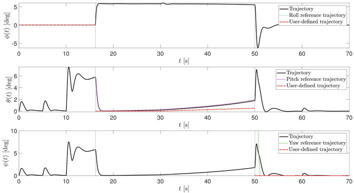
In this section, we illustrate the applicability of the proposed results by means of a numerical simulation. In this simulation, the UAV is tasked with ascending and moving at a constant velocity along the $X$-axis of the inertial reference frame for $t\in \left[0,5\right]$ s, hovering for $t\in \left[5,10\right]$ s, following an upward spiral trajectory for $t\in \left[10,30\right]$ s, descending along the same spiral for $t\in \left[30,50\right]$ s, translating along the bissetriz of the horizontal plane at a constant velocity for $t\in \left[50,60\right]$ s, and hovering until the end of the mission. Furthermore, the user requires that the UAV’s yaw, pitch, and roll angles follow predefined trajectories within a margin of 5 degrees at all times. The user-defined yaw and roll angles are constant at all times, and the user-defined pitch angle is linearly increasing in the ascending and descending phases of the spiral trajectory and constant everywhere else; for details, see Figure 1. It is worthwhile to remark that this reference attitude poses a significant challenge. Indeed, as discussed in Sections 6.2 and 6.3, if $\sigma =2$, that is, if the feedback linearizing output comprises the UAV’s position and pitch angle, then the roll angle can not be equal to zero, Similarly, if $\sigma =1$, that is, if the feedback linearizing output comprises the UAV’s position and roll angle, then the pitch angle can not be set to zero. Furthermore, to follow the reference spiral trajectory imposed by the user, the roll and pitch angles must vary sinusoidally.

Figure 1.

Euler angles capturing the attitude of the UAV. At $t=0$ s, the feedback linearizing output is set as $\sigma =1$. At $t=16.0953$ s, shortly after the UAV is tasked with hovering, applying Algorithm 1, the control system switches feedback linearizing output to $\sigma =2$. Finally, at $t=50.0362$ s, before the UAV is tasked with moving sideways in the horizontal plane, applying Algorithm 1, the control system sets $\sigma =3$. In this stage, after a brief transient, the yaw angle closely follows its reference trajectory.

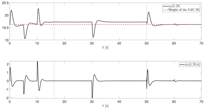
Figure 2 shows the thrust force and the time derivative of the thrust force needed by the UAV to follow the user-defined trajectory. Both $u_1\left(t\right)$, $t\ge 0$, and ${\dot{u}}_1\left(t\right)$ show profiles that are compatible with the performances of commercial-off-the-shelf electric motors for Class 1 quadcopter UAVs.

Figure 2.

Total thrust and time derivative of the total thrust. The total thrust and its derivative lie within bounds that are typical for commercial-off-the-shelf motors of Class 1 quadcopter UAVs.

In this simulation, the UAV’s mass is $m=2$ kg and its central matrix of inertia is given by $I=diag\left(\mathrm{0.010,0.010,0.015}\right)$ kg m². The matrix of aerodynamic coefficient is set equal to $C_{\mathrm{D}}=0.001\cdot {\mathbf{1}}_3$. The estimated mass is $2.2$ kg and the estimated matrix of inertia is given by $diag\left(\mathrm{0.020,0.015,0.025}\right)$ kg m². The adaptive rate matrix is set as ${\mathrm{\Gamma }}_{\sigma }=9\cdot {10}^2\cdot {\mathbf{1}}_{22}$ for all $\sigma \in \left\{\mathrm{1,2,3}\right\}$. We set

$$B_r=\left[\begin{array}{cc}{\mathbf{1}}_3& 0_3\\ \left[\begin{array}{ccc}1& 1& 1\end{array}\right]& 1\end{array}\right],B_{y,\sigma }=\left[\begin{array}{ccc}1& 1& 1\end{array}\right],$$E71

and both ${\tilde{A}}_r$ and ${\tilde{A}}_{y,\sigma }$ were designed through the pole placement method, imposing eigenvalues $\left\{-4.7,-5,-2.5,-2.6,-2.9,-8,-1.21,-2.3,-1.6,-1.8,-1.5,-1.6\right\}$ for the translational dynamics, eigenvalues $\left\{-4,-7\right\}$ for $\sigma =3$ and eigenvalues $\left\{-4,-8\right\}$ for $\sigma \in \left\{1,2\right\}$. The $\sigma$-modification of the MRAC, that is, the adaptive law (22) is employed with ${\gamma }_{\sigma }=0.01$ for all $\sigma \in \left\{\mathrm{1,2,3}\right\}$.

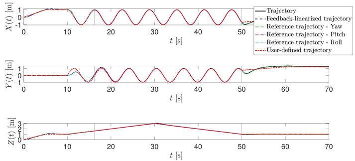
Figure 3 shows the UAV trajectory as a function of time. It is apparent how the UAV closely follows the reference trajectory at all times. Figure 1 shows the UAV attitude by means of the yaw, pitch, and roll angles. The reference angle as well as the user-defined angle are shown only for those stages in which the mode is active. At $t=0$ s, the feedback linearizing output is set as $\sigma =1$. At $t=16.0953$ s, shortly after the UAV is tasked with hovering, applying Algorithm 1, the control system switches feedback linearizing output to $\sigma =2$. Finally, at $t=50.0362$ s, before the UAV is tasked with moving sideways in the horizontal plane, applying Algorithm 1, the control system sets $\sigma =3$. In this stage, after a brief transient, the yaw angle closely follows its reference trajectory. Numerical evidence show that, without the proposed hybrid system, this maneuver would not be possible by setting $\sigma \left(t\right)\equiv 1$ or $\sigma \left(t\right)\equiv 2$ for all $t\ge 0$, that is, without the proposed control system.

Figure 3.

Trajectory of the center of mass of the UAV as a function of time. In all modes, the vehicle’s trajectory closely follows the user-defined trajectory despite uncertainties and the drag force.

8. Conclusion

This chapter presented the first robust MRAC system applicable to time-varying, hybrid plant models affected by parametric, matched, and unmatched uncertainties in the continuous-time dynamics as well as uncertainties in the discrete-time dynamics. These results have been applied to the problem of controlling the feedback-linearized dynamics of a quadcopter UAV and tasking the vehicle to follow both a user-defined trajectory and a user-defined attitude. This result is unprecedented because, due to the UAV’s underactuation, existing works on the control of quadcopters allow regulating arbitrarily only four of its six degrees of freedom. The proposed approach, instead, allows the user to impose reference trajectories for each of the UAV’s six degrees of freedom. Future work directions concern the extension of the proposed approach from a specific application, namely quadcopter UAVs, to generic plant models.

Future work directions involve further extensions of the proposed hybrid MRAC framework for the control of output-feedback linearized systems to cases wherein the feedback-linearizing output is affected by noise. Additional work directions include problems wherein the feedback-linearizing output is not readily available for measurement but needs to be deduced from the measured output.

Acknowledgments

This research was in part performed with the support of NSF through the Grant no. 2137159 and the US Army Research Lab under Grant no. W911QX2320001.

Conflict of interest

The authors declare no conflict of interest.

Abbreviations

MRAC	model reference adaptive control
UAV	unmanned aerial vehicle

References

1. 1. Cortes J. Discontinuous dynamical systems. IEEE Control Systems Magazine. 2008;28(3):36-73
2. 2. Anderson RB, Marshall JA, L’Afflitto A, Dotterweich JM. Model reference adaptive control of switched dynamical systems with applications to aerial robotics. Journal of Intelligent & Robotic Systems. 2020;100(3):1265-1281
3. 3. Lin H, Antsaklis P. Hybrid Dynamical Systems: Fundamentals and Methods, Ser. Advanced Textbooks in Control and Signal Processing. London, UK: Springer; 2021
4. 4. L'Afflitto A. AfflittoModel reference adaptive control for nonlinear time-varying hybrid dynamical systems. International Journal of Adaptive Control and Signal Processing. 2023;37(8):2162-2183
5. 5. Narendra K, Annaswamy A. A new adaptive law for robust adaptation without persistent excitation. IEEE Transactions on Automatic Control. 1987;32(2):134-145
6. 6. Ioannou P, Kokotovic P. Adaptive Systems with Reduced Models. New York, NY: Springer; 1983
7. 7. Ioannou P, Fidan B. Adaptive Control Tutorial. Philadelphia, PA: Society for Industrial and Applied Mathematics; 2006
8. 8. Isidori A. Nonlinear Control Systems. New York, NY: Springer; 1995
9. 9. Malo Tamayo AJ, Villaseñor Rios CA, Ibarra Zannatha JM, Orozco Soto SM. Quadrotor Input-Output Linearization and Cascade Control. IFAC-PapersOnLine. 2018;51(13):437-442. ISSN: 2405-8963. DOI: 10.1016/j.ifacol.2018.07.317
10. 10. Lotufo MA, Colangelo L, Novara C. Control design for uav quadrotors via embedded model control. Transactions on Control Systems Technology. 2020;28(5):1741-1756
11. 11. Daga GD, Thosar AG. Feedback linearization of quadrotor. In: Shrivastava V, Bansal JC, Panigrahi BK, editors. Power Engineering and Intelligent Systems. Singapore: Springer; 2024. pp. 137-151
12. 12. PX4 Website. Available from: https://px4.io/ [Accessed: February 12, 2024]
13. 13. Ardupilot Website. Available from: https://ardupilot.org/ [Accessed: February 12, 2024]
14. 14. Kreyszig E. Introductory Functional Analysis with Applications. New York, NY: Wiley; 1989
15. 15. Bernstein DS. Matrix Mathematics: Theory, Facts, and Formulas. 2nd ed. Princeton, NJ: Princeton University Press; 2009
16. 16. Haddad WM, Chellaboina VS, Nersesov SG. Impulsive and Hybrid Dynamical Systems: Stability, Dissipativity, and Control. Princeton, NJ: Princeton; 2014
17. 17. Sanfelice RG, Goebel R, Teel AR. Generalized solutions to hybrid dynamical systems. Control, Optimisation and Calculus of Variations. 2008;14(4):699-724
18. 18. Bardi M, Capuzzo-Dolcetta I. Optimal Control and Viscosity Solutions of Hamilton-Jacobi-Bellman Equations. Boston, MA: Birkhäuser; 2008
19. 19. Clarke FH. Optimization and Nonsmooth Analysis. Philadelphia, PA: Society of Industrial and Applied Mathematics; 1989
20. 20. Fischer N, Kamalapurkar R, Dixon WE. LaSalle-Yoshizawa corollaries for nonsmooth systems. IEEE Transactions on Automatic Control. 2013;58(9):2333-2338
21. 21. Goebel R, Sanfelice R, Teel A. Hybrid Dynamical Systems: Modeling, Stability, and Robustness. Princeton University Press; 2012. Available form: http://www.jstor.org/stable/j.ctt7s02z. ISBN: 9780691153896
22. 22. Khalil HK. Nonlinear Systems. Princeton, NJ: Prentice Hall; 2002
23. 23. Pomet JB, Praly L. Adaptive nonlinear regulation: estimation from the Lyapunov equation. IEEE Transactions on Automatic Control. 1992;37(6):729-740
24. 24. Lavretsky E, Wise K. Robust and Adaptive Control: With Aerospace Applications. London, UK: Springer; 2012
25. 25. Ioannou P, Sun J. Robust Adaptive Control, Ser. Dover Books on Electrical Engineering Series. Upper Saddle River, NJ: Dover Publications; 2012
26. 26. L’Afflitto A, Anderson RB, Mohammadi K. An introduction to nonlinear robust control for unmanned quadrotor aircraft. IEEE Control Systems Magazine. 2018;38(3):102-121
27. 27. L’Afflitto A. A Mathematical Perspective on Flight Dynamics and Control. London, UK: Springer; 2017
Written By
Giri M. Kumar, Mattia Gramuglia and Andrea L’Afflitto
Submitted: 30 January 2024 Reviewed: 02 February 2024 Published: 02 April 2024