A Fixed-Bed Column Sorption: Breakthrough Curves Modeling

Abstract

Global attention has increasingly focused on environmental pollution due to its widespread and devastating impact. The urgency of addressing climate change has propelled it to the forefront of governmental agendas worldwide, emphasizing the need for actions to secure a pollution-free future. Pollution treatment methods have consequently gained global significance, with adsorption emerging as a particularly relevant approach, especially in developing economies. Adsorption proves to be a cost-effective, safe, efficient, and easily manageable method that can utilize low-cost or waste materials. In designing treatment systems based on adsorption, batch tests are crucial, employing adsorption isotherms such as Langmuir and Freundlich to understand the phenomenon. While equilibrium points are essential in some situations, continuous processes benefit from column implementations, where a fundamental understanding of breakthrough curves becomes pivotal. Various adsorption kinetic models, such as the Thomas model, Adams–Bohart model, Yoon–Nelson model, and bed-depth/service time (BDST) model, explain and determine breakthrough curves. The assessment of these models for compatibility with experimental data and model-generated data is essential. Criteria such as Mean Relative Error (MRE) and Normalized Relative Mean Square Error (NRMSE) are commonly employed to objectively select the most suitable model for a given scenario.

1. Introduction

Bois-Reymond initially proposed the concept of “adsorption”, but was later introduced to the scientific community by Kayser. It is defined as the accumulation of a specific compound at the interface between two phases, this phenomenon involves the transfer from one phase to the other and subsequently adheres to the surface. This process is considered intricate and largely influenced by the surface chemistry or the characteristics of the sorbent, sorbate, and the environmental conditions between the two phases [1]. This procedure can be efficiently employed to move contaminants or pollutants from wastewater and concentrate them on the surface of adsorbents [2]. Certain compounds undergo transportation from one phase to another before adhering to a surface. This process is regarded as a complex phenomenon primarily reliant on the surface chemistry or characteristics of the sorbent and sorbate, as well as the system conditions between the two phases [1].

The material that gets adsorbed onto the surface of another substance is termed the adsorbate. Meanwhile, the substance existing in bulk, where this adsorption occurs on the surface, is known as the adsorbent. This interaction can manifest at interfaces such as liquid-liquid, liquid-solid, gas-liquid, or gas-solid. Among these types, it is primarily liquid-solid adsorption that finds extensive application in water and wastewater treatment [1]. The process consists of a sequence of four steps, during which the dissolved substance (adsorbate) undergoes transitions to reach the boundary layer and adheres to the adsorbent. The following four stages describe the movement of the solute (adsorbate) toward the boundary layer and its binding to the adsorbent:

1. Advective transport: Dissolved particles are transported from the overall solution to an immobilized film layer through advective flow, axial dispersion, or diffusion.

2. Film transfer: Solute particles permeate the immobile water film layer and accumulate within it.

3. Mass transfer: Solute particles gather on the surface of the adsorbent.

4. Intraparticle diffusion: The solute undergoes movement into the pores of the adsorbent [1].

Sorption is initiated by the concentration difference between the liquid and the surface of the adsorbing solid. During this phase, the movement of solute molecules is solely guided by molecular diffusion across the interface. The functional groups within the adsorbent solid determine the affinity and the type of interaction with the adsorbed molecules. The binding of these molecules to the adsorbent causes a change in entropy, specifically, a decrease in entropy [2].

There exist two primary types of adsorption: Physical adsorption is instigated by weak Van der Waals forces of attraction. This type of adsorption is reversible and is distinguished by low enthalpy values, typically around 20 kJ mol⁻¹. In physical adsorption, the attractive forces between the adsorbed molecules and the solid surface are feeble, allowing the molecules to move freely across the surface rather than being firmly attached to a specific location on the adsorbent surface. Electrostatic forces, such as dipole-dipole interactions, dispersion forces, and hydrogen bonding, play a role in the interactions between the adsorbate and adsorbent in physical adsorption [1, 2].

On the other hand, chemisorption involves chemical bonding between the sorbate and sorbent molecules. This type of sorption is irreversible and exhibits a higher enthalpy of sorption, around 200 kJ mol⁻¹. In chemisorption, the attraction between the sorbent and sorbate is pivotal, and this is facilitated by more robust electrostatic forces, including covalent or electrostatic chemical bond [1, 2]. The ranges of energy for each reactions are: (II) Van der Waals force 4 < enthalpy <10 kJ mol⁻¹, (II) Hydrophobic Force <5 kJ mol⁻¹, (II) Dipole Force 2 < enthalpy <29 kJ mol⁻¹, (IV) Hydrogen Bond 2 < enthalpy <40 kJ mol⁻¹, (V) Coordination Exchange 40 < enthalpy <60 kJ mol⁻¹, and (VI) Chemical Bond Enthalpy >60 kJ mol⁻¹ [1, 2]. The accumulation of pollutants in the environment is a product of human activities, such as mining and the discharge of industrial waste [3]. One of the most promising technologies for treating large volumes of diluted pollutants in solutions is sorption [4]. Sorption describes a mass transfer process, where a dissolved material is transferred directly to the surface of the solid phase, after it is bound by chemical and/or physical interactions [5]. The sorption capacity of a material obtained from batch studies presents useful results to know the effectiveness of a sorption system, however, this information is generally not applicable to most treatment systems where the time of contact is not enough to reach equilibrium, therefore, there is a need to perform equilibrium studies using columns [3]. The batch operation mode is straightforward, employing a consistent volume approach, making it simple to operate. Conversely, the continuous flow operation, with varying volumes, is somewhat more complex, necessitating additional devices like pumps, flow regulators, strainers, temperature controllers, and so on. Batch processing is suitable for initial research endeavors to explore isotherms and kinetics. Meanwhile, continuous flow studies delve into a comprehensive understanding of the dynamics of biosorption processes during large-scale operations [2]. The fixed-bed adsorption column systems allow to determine the maximum performance of the adsorbent materials and to identify the best dynamic operating conditions (6). Fixed-bed column adsorption has many advantages due to its simple operation and high removal efficiency [6]. Understanding breakthrough curves is essential in designing a continuous flow system for the adsorption of pollutants. Typically, this information is obtained through experimental determination or modeling, relying on kinetic behavior and the isothermal model [7].

The continuous operation of a fixed-bed column adsorption process serves as a crucial link between laboratory experimentation and real-world applications, offering valuable insights. Nevertheless, optimizing operational parameters through direct column experimentation, specifically with limited data points, can be an arduous, time-consuming, and costly endeavor. Hence, numerous mathematical models have been devised to predict actual adsorption behaviors and deliver effective design insights for columns, negating the need for physical experimentation [8]. Adsorption can be conducted in both batch and continuous modes. Batch adsorption experiments are crucial for collecting fundamental data regarding pollutant removal through adsorption. However, to effectively apply this process in wastewater treatment, continuous adsorption studies are indispensable for practical implementation [9]. In general, continuous adsorption is carried out with a fixed-bed column where wastewater encounters a stationary bed of adsorbent. In this continuous adsorption process, the wastewater constantly enters and exits the column, maintaining a dynamic equilibrium. This equilibrium is upheld as the concentration of ions in both the solution and the adsorbent within the column is constantly changing [9].

In experiments involving a fixed-bed column, a specific amount of untreated or pre-treated biosorbents within a solid matrix is densely packed into a column of defined length. The column is equipped with sieves at the bottom to prevent the biosorbent from being carried away by the liquid phase. This loaded column is then placed in a thermostat to maintain a constant temperature and is connected to a positive displacement pump, often a peristaltic pump, with a flow regulator. The liquid phase, containing dissolved substances (contaminants), flows through the fixed-bed column at a predetermined rate.

As the fixed-bed becomes wet, dissolved substances move out of the liquid phase and adhere to the surface of the stationary matrix due to their affinity. This translocation and binding of solute molecules persist until the pores or functional groups of the biosorbents reach equilibrium. Once saturation is attained, further adsorption becomes impractical, and the transfer of solute at the solid-liquid interface ceases. Additionally, the transfer of solutes across the phase boundary encounters diffusion resistance from the surrounding film and within the particles.

The adsorbed molecules necessitate a sufficient amount of time to remain in the column. The residence or retention time is contingent on the volumetric flow rate of the liquid samples and is, therefore, a crucial parameter for the optimal design of the continuous biosorption process [2].

The effectiveness of continuous adsorption is assessed by evaluating parameters such as column efficiency in removing contaminants, column uptake capacity, and breakthrough curve profile. These parameters are influenced by operating factors such as the bed diameter, bed depth, flow rate, and initial concentration of the contaminant [9].

2. Adsorption models for column study

2.1 Calculation of the dynamic adsorption parameters

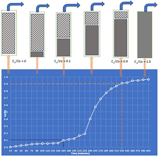
The performance of an adsorption column can be determined according to breakthrough curves (Figures 1 and 2). The duration of breakthrough occurrence and the configuration of the breakthrough curve are crucial attributes for assessing the operation and dynamic response of a sorption column [10, 11].

Figure 1.

Representation of breakthrough curve.

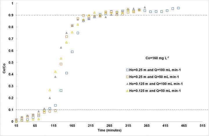
Figure 2.

Behavior of a breakthrough curve, when the initial concentration remains constant, varying the height of the column (H₀) and the flow rate (Q).

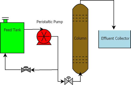
Figure 3 shows a scheme for a continuous adsorption process. This scheme can be used for a laboratory experiment or for a larger scale such as a pilot plant. To regulate the fed flow, an arrangement of valves can be used to return part of the flow to the feed tank.

Figure 3.

Schematic illustrator continuous adsorption process.

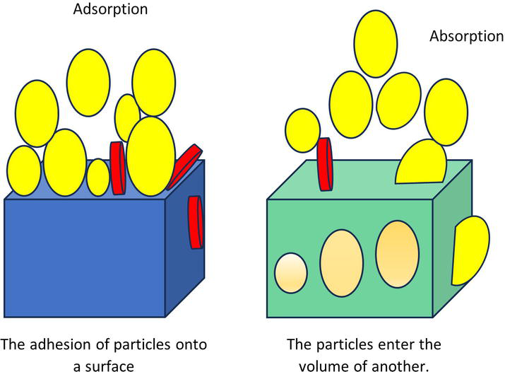
Figure 1 shows the diagram of the development of the adsorption process and the representation of the breakthrough curve as well as a diagram of the saturation process of the material with which the column was packed. The darkest part of the column illustrates how the material becomes saturated over time (Figure 4).

Figure 4.

Scheme of the adsorption process.

The breakthrough point is typically reached when the effluent concentration (C_e) from the column reaches around 5 to 10% of the influent concentration (C₀) [10, 11]. The point where the effluent concentration reaches 90% is usually called the “point of column exhaustion” [10, 11]. By plotting C_e/C_o versus the reaction time, the breakthrough curves for an adsorbent will be obtained under certain conditions. The effluent volume, V_eff (mL), can be calculated from the following equation [8, 10, 11]:

$$V_{\mathit{eff}}=Q{t}_{\mathit{\text{total}}}$$E1

Where: Q is the volumetric flow rate (mL min⁻¹), and t_total is the total flow time (min). For a given flow rate and influent concentration, the maximum adsorption capacity of column, q_total (mg), is obtained using [8, 10, 11, 12, 13]:

$$q_{\mathit{\text{total}}}=\frac{\mathit{QA}}{1000}=\frac{Q}{1000}{\int }_{t=0}^{t=t_{\mathit{\text{total}}}}{C}_t\mathit{dt}$$E2

$$q_e=\frac{q_{\mathit{\text{total}}}}{m}$$E3

Where: A is the area column cross-section area (cm²), C_t ion concentration after time t (mg L⁻¹), q_e is maximum capacity of the column (mg of pollutant g⁻¹ Adsorbent), m is the mass of adsorbent in the column (g), Q is the volumetric flow rate (mL min⁻¹), and t_total is the total flow time (min).

Arranging the Eqs. (2) and (3), obtained [3, 8, 10, 11, 12, 13, 14]:

$$q_e=\frac{C_{0}Q}{m\ast 1000}\underset{t=0}{\overset{t=t_{\mathit{\text{total}}}}{\int }}\left(1-\frac{C_e}{C_0}\right)\mathit{dt}$$E4

The total quantity of ions entering the column (m_total) is computed using the following Eq. (17):

$$m_{\mathit{\text{total}}}=\frac{C_{0}Q{t}_{\mathit{\text{total}}}}{1000}$$E5

The total pollutant ions getting into the fixed-bed W (mg) can be calculated from the following equation [8, 12, 14]:

$$W=C_{0}F{t}_e$$E6

Where: F is the volumetric flow rate (mL h⁻¹) and t_e is the exhaustion time (h).

Total removal percent of ions can be calculated from [12, 13, 14]:

$$Y\%=\frac{q_{\mathit{\text{total}}}}{W_{\mathit{\text{total}}}}\ast 100$$E7

The flow rate represents the empty bed contact time (EBCT) in the column, as described in [10]:

$$\mathit{\text{EBCT}}\left(min\right)=\frac{\mathrm{Bed}\text{volume}\left(\mathrm{mL}\right)}{\text{Flow rate}\left(\mathrm{mL}/min\right)}$$E8

Typically, the breakthrough time on the curve is defined as the moment when the contaminant concentration in the effluent reaches the specified limit standard or a predetermined fraction of the initial concentration [8]. The breakthrough time (t_b) refers to the point at which 10% of the initial concentration is detected in the effluent concentration, known as the concentration breakthrough (C_b), and is closely related to the Fraction Bed Utilization (FBU) [6, 15].

$$C_b=0.1C_0$$E9

$$C_S=0.9C_0$$E10

$$\mathit{FBU}=\frac{q_b}{q_s}$$E11

$$q_b=\frac{C_{0}Q}{1000m}\underset{0}{\overset{t_b}{\int }}\left(1-\frac{C_b}{C_0}\right)$$E12

$$q_s=\frac{C_{0}Q}{1000m}\underset{0}{\overset{t_s}{\int }}\left(1-\frac{C_s}{C_0}\right)$$E13

Where: $C_b$ is breakthrough concentration (mg L⁻¹), $C_S$ is saturation concentration (mg L⁻¹), $q_b$ is the amount of ions adsorbed at breakthrough time (mg g⁻¹), $q_s$ is the amount of ions adsorbed at saturation time (mg g⁻¹), $t_b$ is breakthrough time (min), and $t_s$ is saturation time (min).

2.2 Adsorption kinetic models

Effectively designing a column adsorption process necessitates accurately predicting the breakthrough curve in the effluent. Throughout the years, numerous straightforward mathematical models have been created to describe and analyze laboratory-scale column studies, catering specifically to industrial applications [10, 11].

2.2.1 Thomas model

The model assumes that there is no axial diffusion when passing the solution through the filling material of the column and the kinetic model of Pseudo-second order is the one that best describes the adsorption process [11, 13, 16]. The equation that describes it is the following:

$$\frac{C_e}{C_o}=\frac{1}{1+\mathit{exp}\left[\frac{K_{\mathit{Th}}{q}_{e}m}{Q}-K_{\mathit{Th}}{C}_{0}t\right]}$$E14

Its linear form is expressed as:

$$\mathit{Ln}\left[\frac{C_0}{C_e}-1\right]=\frac{K_{\mathit{Th}}{q}_{e}m}{Q}-K_{\mathit{Th}}{C}_{0}t$$E15

Where C_e is the effluent ions concentration (mg L⁻¹); C₀ is initial ions concentration (mg L⁻¹); Q is flow rate (L h⁻¹); qe is the equilibrium column capacity (mg g⁻¹); m is the weight of Zeolite in column (g); K_Th is the Thomas model constant (mL min⁻¹ mg⁻¹), and t stands for total flow time (min).

The values of K_Th and q_e can be determined from the linear plot of Ln[(C_o/C_e)-1] against t [10, 13, 16].

2.2.2 Bohart and Adams model

In this model, it is assumed that the rate of adsorption is directly proportional to both the concentration of the adsorbate and the remaining capacity of the adsorbent for the adsorbate [11]. This model adds that the equilibrium is not instantaneous and, therefore, is used to model the initial part of the breakthrough curves. Based on the surface reaction theory, established a fundamental equation, which describes the relationship between Ce/C₀ and t in a continuous system.

The equation that describes it is the following [11]:

$$\frac{C_e}{C_0}=\frac{exp\left(K_{\mathit{BA}}·C_0·t\right)}{exp\left(K_{\mathit{BA}}·q_{\mathit{max}}·\frac{Z}{U_0}\right)-1+\mathit{exp}\left(K_{\mathit{BA}}·C_0·t\right)}$$E16

The linear expression is as follows [16, 17]:

$$\mathit{Ln}\frac{C_e}{C_0}=K_{\mathit{AB}}{C}_{0}t-K_{\mathit{AB}}{N}_0\left(\frac{Z}{U_0}\right)$$E17

Where: C₀ and Ce are the influent and effluent concentration (mg L⁻¹), respectively; K_AB is the kinetic constant (L mg⁻¹ min⁻¹), t breakthrough time min, q_max maximum adsorption capacity (mg ions g⁻¹ absorbent), N₀ is the saturation concentration (mg L⁻¹), Z is the bed depth of the fix-bed column (cm), and U₀ is the superficial velocity (cm min⁻¹) defined as the ratio of the volumetric flow rate Q (cm³ min⁻¹) to the cross-sectional area of the bed A (cm²).

The parameters K_AB and N₀ can be calculated from the linear plot of ln (Ce/C₀) against t [10].

2.2.3 Yoon-Nelson model

The Yoon-Nelson model stands out for its straightforward equation notation in contrast to other mathematical models that have been examined. Its fundamental assumption is that the reduction in the rate of adsorption for an adsorbate molecule is directly proportional to the adsorption of the adsorbate and the breakthrough of the adsorbent bed [11]. It assumes that the rate of decay in the probability of adsorption for the adsorbate molecule is proportional to the adsorption of the adsorbate probability and the probability of breakthrough of the adsorbate on the adsorbent [10], and is applicable for a single component system [16]. The nonlinear equation that describes it is the following:

$$\frac{C_e}{C_0}=\frac{e^{k_{\mathit{YN}}\ast \left(t-\tau \right)}}{1+e^{k_{\mathit{YN}}\ast \left(t-\tau \right)}}$$E18

The linearized Yoon-Nelson model for a single component system can be expressed as [11]:

$$\mathit{Ln}\frac{C_e}{C_0-C_e}=K_{\mathit{YN}}t-\tau K_{\mathit{YN}}$$E19

Where: K_YN is the rate constant (min⁻¹) and $\tau$ is the time required for 50% adsorbate breakthrough (min).

A linear plot of ln [Ce/(C₀-Ce)] against t determined the values of K_YN and $\tau$ from the slope and intercept, respectively [8, 10, 16].

2.2.4 The bed-depth/service time (BDST) model

Hutchins in 1973 linearized the model introduced in 1920 by Bohart and Adams. This linearization led to the development of the widely adopted and highly recommended BDST design model. Many authors have since endorsed it as the most straightforward and fastest means of predicting adsorbent performance [17].

The BDST model is employed to describe the characteristics of a column with a consistent bed height. It includes an equation for the duration of operation concerning the deposit depth, which enables the construction of a graph illustrating the relationship between the operation time (t) and the ratio C_t/C₀. This graphical representation facilitates the determination of the dynamic parameters of the BDST model [8, 11].

It is expressed as follows:

$$\mathrm{t}=\frac{N_0}{C_{0}F}Z-\frac{1}{K_a{C}_0}\mathit{Ln}\left(\frac{C_0}{C_t}-1\right)$$E20

where: N₀ is the weight of ions adsorbed per unit weight of adsorbate; C₀ is the influent concentration (mg L⁻¹); C_t is ions concentration at breakthrough point (mg L⁻¹); Z is the bed depth (cm); F is the linear velocity (cm h⁻¹); and K_a is the rate constant (L mg⁻¹ h⁻¹) [12, 17].

Hutchins expressed the Bohart-Adams equation as a linear equation [12, 13, 17, 18]:

$$t=\mathit{aZ}-b$$E21

Where:

$$a=\frac{N_0}{C_{0}F}$$E22

$$b=\frac{1}{K_a{C}_0}\mathit{Ln}\left(\frac{C_0}{C_t}-1\right)$$E23

Where: The slope a corresponds to Eq. (22) and the intercept b to Eq. 23.

[3, 10, 12, 14, 17, 19, 20, 21, 22].

2.2.5 Wolborska model

The Wolborska Model, introduced by Wolborska in 1989, presents an equation that examines the mass transfer of diffusion in breakthrough curves within a low concentration range. The model’s equation is depicted as follows:

$$\mathit{ln}\left(\frac{C_t}{C_0}\right)=\frac{\beta C_{0}t}{N_0}-\frac{\mathit{\beta Z}}{U_0}$$E24

Where $\beta$ is the external mass transfer coefficient min⁻¹. $N_0$ is the adsorption capacity of the bed per unit volume (mg L⁻¹).

The values of the parameters of the Wolborska model can be determined from the Plot of $\mathit{ln}\left(\frac{C_t}{C_0}\right)$ versus time [23, 24].

2.2.6 Yan et al. model

It overcame the constraint of Thomas’s model related to the outlet concentration specifically at time (t = 0).

$$\mathit{ln}\left(\frac{C_t}{C_0-C_t}\right)=\frac{K_Y{C}_0}{Q}\mathit{ln}\left(\frac{Q^2}{K_Y{q}_{Y}m}\right)+\frac{K_Y{C}_0}{Q}\mathit{lnt}$$E25

The values of model parameters are evaluated from the linearized plot between $ln\left(\frac{C_t}{C_0-C_t}\right)$ and ln t [1, 24].where K_Y mL mg⁻¹ min⁻¹, q_Y mg g⁻¹.

2.2.7 Modified dose-model (MDR)

This model has found widespread application in pharmacology, serving to characterize various processes. Presently, it is applied in delineating column biosorption processes, valued for its precision in depicting the full breakthrough curve while reducing errors, particularly those stemming from the Thomas model, especially in scenarios involving low or high removal times [24]. This model is expressed by:

$$\mathit{ln}\left(\frac{C_t}{C_0-C_t}\right)=a\mathit{ln}\left(C_0{Q}_t\right)-a\mathit{ln}\left(q_{\mathit{mdr}}m\right)$$E26

By plotting $\mathit{ln}\left(\frac{C_t}{C_0-C_t}\right)$ against time t, we extract the model parameters, a and $q_{\mathit{mdr}}$, from the slope and the intercept, respectively. Here, a denotes the model constant, while $q_{\mathit{mdr}}$ signifies the maximum concentration of solute in the solid phase (mg g⁻¹) [24].

The linearized plots of $\mathit{ln}\left(\frac{C_t}{C_0-C_t}\right)$ versus $ln\left(C_0{Q}_t\right)$

2.2.8 Clark model

It coupled mass transfer with the Freundlich isotherm. This model is expressed by:

$$\mathit{lnA}-\mathit{rt}=\mathit{ln}\left({\left(\frac{C_t}{C_0}\right)}^{1-n}-1\right)$$E27

Values of n required for the above model are acquired from the data of Freundlich isotherm. Linearized plots of $\mathit{ln}\left({\left(\frac{C_t}{C_0}\right)}^{1-n}-1\right)$ versus t [24].

Table 1 presents the models, their equation in linear form, and the main characteristics of the models.

Models	Equation linear form	Main characteristics of the model	References
Thomas Model	$\mathit{Ln}\frac{C_e}{C_0}=K_{\mathit{AB}}{C}_{0}t-K_{\mathit{AB}}{N}_0\left(\frac{Z}{U_0}\right)$	kinetic model of Pseudo-second order.	[10, 11, 13, 16]
Bohart and Adams Model	$\mathit{Ln}\left[\frac{C_0}{C_e}-1\right]=\frac{K_{\mathit{Th}}{q}_{e}m}{Q}-K_{\mathit{Th}}{C}_{0}t$	Assumed direct proportionality between adsorption rate and adsorbate concentration.	[10, 11]
Yoon-Nelson model	$\mathit{Ln}\frac{C_e}{C_0-C_e}=K_{\mathit{YN}}t-\tau K_{\mathit{YN}}$	The decrease in adsorption rate is linked to both adsorbate adsorption and breakthrough in the adsorbent bed.	[8, 10, 16]
The bed-depth/service time (BDST) model	$t=\mathit{az}-b$	Linearized the model by Bohart and Adams	[3, 10, 12, 14, 17, 19, 20, 21, 22]
	$a=\frac{N_0}{C_{0}F}$
	$b=\frac{1}{K_a{C}_0}\mathit{Ln}\left(\frac{C_0}{C_t}-1\right)$
Wolborska Model	$\mathit{ln}\left(\frac{C_t}{C_0}\right)=\frac{\beta C_{0}t}{N_0}-\frac{\mathit{\beta Z}}{U_0}$	Mass transfer of diffusion in breakthrough curves within a low concentration range.	[23, 24]
Yan et al. Model	$\mathit{ln}\left(\frac{C_t}{C_0-C_t}\right)=\frac{K_Y{C}_0}{Q}\mathit{ln}\left(\frac{Q^2}{K_Y{q}_{Y}m}\right)+\frac{K_Y{C}_0}{Q}\mathit{ln}t$	It addressed the limitation in Thomas’s model concerning initial outlet concentration at time (t = 0).	[1, 24]
Modified Dose–Response Model (MDR)	$\mathit{ln}\left(\frac{C_t}{C_0-C_t}\right)=a\mathit{ln}\left(C_0{Q}_t\right)-a\mathit{ln}\left(q_{\mathit{mdr}}m\right)$	Widespread application in pharmacology	[24]
Clark Model	$\mathit{ln}A-\mathit{rt}=\mathit{ln}\left({\left(\frac{C_t}{C_0}\right)}^{1-n}-1\right)$	It coupled mass transfer with the Freundlich isotherm	[24]

Table 1.

Adsorption models for column study.

2.3 Evaluation criteria

To evaluate and compare the experimental and calculated results of C_e/C_o for the dynamic adsorption of ions in a packed bed column system, applied Mean Relative Error (MRE) and Normalized Relative Mean Square Error (NRMSE) statistical criteria. These criteria are described as follows [25]:

$$\mathrm{MRE}=\frac{{\sum }_{\mathrm{i}=1}^{\mathrm{n}}\left[{\left(\frac{{\mathrm{C}}_{\mathrm{e}}}{{\mathrm{C}}_0}\right)}_{\mathrm{cal}}-{\left(\frac{{\mathrm{C}}_{\mathrm{e}}}{{\mathrm{C}}_0}\right)}_{\exp }\right]}{\mathrm{n}{\left(\overline{\frac{{\mathrm{C}}_{\mathrm{e}}}{{\mathrm{C}}_0}}\right)}_{\exp }}$$E28

Where:

cal is calculated and exp. obtained experimentally.

$$\mathit{\text{NRMSE}}={\left[\frac{{\sum }_{\mathrm{i}=1}^{\mathrm{n}}{\left[{\left(\frac{{\mathrm{C}}_{\mathrm{e}}}{{\mathrm{C}}_0}\right)}_{\mathrm{cal}}-{\left(\frac{{\mathrm{C}}_{\mathrm{e}}}{{\mathrm{C}}_0}\right)}_{\exp }\right]}^2}{\mathrm{n}{\left(\overline{\frac{{\mathrm{C}}_{\mathrm{e}}}{{\mathrm{C}}_0}}\right)}_{\exp }}\right]}^{0.5}\ast 100$$E29

The performance of the numerical model is poor when the NRMSE >30%, fair if the 20% < NRMSE <30%, good if the 10% < NRMSE <20% and excellent if the 0 < NRMSE <10%. In general, the performance of numerical model is acceptable if the NRMSE <30% [25]. For better assessment, the linear regression was fitted between (C_e/C_o)_exp and (C_e/C_o)_cal values by the following equation:

$${\left(\frac{C_e}{C_0}\right)}_{\mathit{exp}}=m{\left(\frac{C_e}{C_0}\right)}_{\mathit{cal}}+n$$E30

Where: m is the slope of line and n is the distance from the origin.

The value of n is considered zero when it is not significant at 5% level [25].

2.4 Thermodynamic study

Thermodynamic parameters serve to assess the orientation and feasibility of the adsorptive reaction. The conjectures regarding the adsorption mechanism rely on the alterations in Gibbs free energy (∆G°), the change in standard enthalpy (∆H°), and the change in standard entropy (∆S°) [26]. These thermodynamic parameters are calculated using the following equations:

$$K_c=\frac{C_A}{C_e}$$E31

$$∆G^0=-\mathit{RT}\mathit{ln}{K}_c$$E32

$$∆G^0=∆H^0-T∆S^0$$E33

$$\mathit{lnK}=\frac{∆S^0}{R}-\frac{∆H^0}{\mathit{RT}}$$E34

$$∆G^0=∆H^0-T∆S^0$$E35

Where: Kc is the adsorption affinity and can be determined by the ratio between the amount adsorbed at equilibrium (C_A mg g⁻¹) and the equilibrium concentration (C_e mg L⁻¹). R is the universal gas constant (8.314 J mol K⁻¹), T is the absolute temperature of the solution (°K). The values of ΔH° and ΔS° are derived from the slope and intercept, respectively, by graphing the Van’t Hoff line on the abscissa axis with 1/T against the ordinate axis with ln kc. Alternatively, one can calculate these parameters by graphing ΔG° against T, where the slope of the resulting straight line corresponds to ΔH°, and the intercept represents ΔS°. Alternatively, these parameters can also be calculated by plotting on the abscissa axis with T versus the ordinate axis with ΔG°, whereby the slope of the resulting straight line corresponds to ΔH°, and the intercept represents ΔS° [6, 26, 27, 28].

Negative values in ΔG° indicate a spontaneous character of the adsorption process. As the values become more negative with increasing temperature, they indicate that the increase in temperature favors the adsorption process. If negative values are given in ΔH°, this indicates that the process is exothermic, while positive values indicate an endothermic process. When positive values are given in ΔS°, they indicate an increase in randomness at the liquid-solid interface of the system during the adsorption process. If the absolute change in Gibbs free energy is between −20 and 0 KJ mol⁻¹, it is generally physical adsorption, whereas for chemical adsorption, it is in the range of −80 to −400 KJ mol⁻¹ [26, 28].

2.4.1 Estimation of activation energy (E_a)

The magnitude of the activation energy provides insight into the nature of the adsorption process, which generally falls into two main categories: physical and chemical adsorption. In activated chemical adsorption, the rate varies with temperature according to a finite activation energy (8.4–83.7 kJ mol⁻¹) in the Arrhenius equation. In the case of non-activated chemical adsorption, the activation energy is close to zero [26, 28]. The activation energy was calculated using the Arrhenius equation:

$$K_c=K_0\mathit{Exp}\left(-\frac{E_a}{\mathit{RT}}\right)$$E36

Where:

k₀ is the temperature-independent rate constant (g mg⁻¹ min⁻¹),

E_a is the apparent activation energy of the adsorption reaction (kJ mol⁻¹). The linear form of the equation is expressed as:

$$\mathit{Ln}{K}_c=-\frac{E_a}{R}\frac{1}{T}+\mathit{Ln}{K}_0$$E37

By plotting ln K_c against 1/T, we will obtain a straight line with a slope equal to -E_a/R [26, 28].

2.5 Scale-up design

Given the resemblances in empty bed contact time (EBCT) and hydrodynamic characteristics between laboratory-scale and pilot/full-scale column systems, it is viable to employ data from the laboratory scale for calculating parameters and modeling the efficiency of larger column systems using vertical scaling techniques. To achieve comparable hydrodynamic properties between laboratory-scale and large-scale column systems, this approach uses the filtration rate (FR) and empty bed contact time (EBCT) values obtained from a laboratory-scale column system as the basic parameters for the design of the larger column system. These relationships are defined by the following equations [15]:

$$\mathit{FR}=\frac{Q_L}{A_L}$$E38

$$A_D=\frac{Q}{\mathit{FR}}$$E39

$$\tau =\frac{V_L}{Q}$$E40

$$H_{\mathit{BD}}=\mathit{FR}\ast \tau$$E41

$$M_D=V_D\ast A_D\ast H_{\mathit{BD}}$$E42

$$B_D=\frac{M_{\mathit{AC}}}{M_{\mathit{CR}}}$$E43

$${\mathit{BV}}_D=B_D\ast Q_D$$E44

Where: FR is the filtration rate (cm min⁻¹), A_D area of the design column (cm²), EBCT of the lab-scale column ($\tau$, min), H_BD bed height of the design column (cm), M_D mass of the adsorbent required in the design column (kg), B_D breakthrough time of the design column (min), BV_D volume treated before breakthrough (m³), Q_L is flow rate in the lab-scale (cm³ min⁻¹), A_L denotes cross-sectional area in the lab-scale (cm²), V_L volume of lab-scale column (cm³), V_D volume of design column (cm³), M_AC is amount of adsorbent consumed in the design column (kg), M_CR is adsorbate consumption rate of the design column (kg d⁻¹), and Q_D is flow rate in the design column (m³ d⁻¹). Since the ratio of the column diameter to the particle diameter is more than twenty, wall effects can be assumed negligible [29].

3. Conclusions

To optimize outcomes when implementing an adsorption-based treatment system, starting with batch experiments is key. These experiments are straightforward and cost-effective, offering preliminary insights into the adsorption traits of a particular material. However, they often fall short in fully establishing an effective treatment process. To achieve this, conducting continuous experiments becomes essential for a more comprehensive understanding of a material’s adsorption behaviors in a continuous setup. Detailed mathematical models designed for this purpose have been extensively developed to elucidate how a material interacts with specific contaminants or a combination thereof. Once results from a laboratory-scale column are obtained, it is advisable to proceed by scaling up and testing using a pilot or semi-pilot plant-scale model to ensure the reliability of the findings.

Verifying the similarity between results derived from mathematical models and those obtained experimentally is crucial. Using evaluation criteria is necessary to ensure a level of certainty regarding the statistical significance and resemblance of the experimental results.

Acknowledgments

Advanced Materials Research Center (CIMAV) and Faculty of Animal Science and Ecology, Autonomous University of Chihuahua.

Conflict of interest

The authors declare no conflict of interest.